Rotationally Induced Local Heat Transfer Features in a Two-Pass Cooling Channel: Experimental–Numerical Investigation ^†

Abstract

Turbine blades for modern turbomachinery applications often exhibit complex twisted designs that aim to reduce aerodynamic losses, thereby improving the overall machine performance. This results in intricate internal cooling configurations that change their spanwise orientation with respect to the rotational axis. In the present study, the local heat transfer in a generic two-pass turbine cooling channel is investigated under engine-similar rotating conditions ($Ro=\{0\dots 0.50\}$) through the transient Thermochromic Liquid Crystal (TLC) measurement technique. Three different angles of attack ($\alpha =\{-{18.5}^{°};+8^{°};+{46.5}^{°}\}$) are investigated to emulate the heat transfer characteristics in an internal cooling channel of a real turbine blade application at different spanwise positions. A numerical approach based on steady-state Reynolds-averaged Navier–Stokes (RANS) simulations in ANSYS CFX is validated against the experimental method, showing generally good agreement and, thus, qualifying for future heat transfer predictions. Experimental and numerical data clearly demonstrate the substantial impact of the angle of attack on the local heat transfer structure, especially for the radially outward flow of the first passage, owing to the particular Coriolis force direction at each angle of attack. Furthermore, results underscore the strong influence of the rotational speed on the overall heat transfer level, with an enhancement effect for the radially outward flow (first passage) and a reduction effect for the radially inward flow (second passage).

1. Introduction

Cooling mechanisms for highly thermally stressed components in modern turbomachinery play an essential role in maintaining temperatures below a specified threshold and thereby guaranteeing their operating life expectancy. However, discharge of pressurized air from the compressor represents a loss of overall gas turbine efficiency and calls for thoughtful application to ensure an optimal performance. In this context, a detailed understanding and reliable prediction of heat transfer characteristics under engine-similar operating conditions will lead to optimized designs with decreased coolant consumption, thereby increasing the thermal efficiency.

In regard to turbines blades, rotation can dramatically affect the secondary flow field within the internal cooling channel. Han [1] highlighted the significance of the two forces that appear in the presence of rotation; on the one hand, the Coriolis force deflects the core flow to the pressure side for a radially outward flow. Counter-rotating vortex pairs develop and drive the fluid back to the suction side along the side walls, as reviewed by Ligrani [2]. Near-wall velocity is increased for the pressure side and decreased for the suction side with the subsequent heat transfer augmentation and reduction on either side. On the other hand, as a result of the temperature difference between channel walls and coolant, which is reduced in the streamwise direction, a centrifugal buoyancy force appears. The latter force is sensitive to the heat flux direction and must be considered in the experimental setup design. The combined effect of both forces results in a much different heat transfer pattern compared to the non-rotating frame.

Rotating cooling channels have been extensively investigated over the past decades through experiments [3,4,5,6,7,8]. Wagner et al. [3] conducted comprehensive investigations on smooth and ribbed multipass configurations by means of heated segments, covering a broad range of Reynolds numbers, rotation numbers, and inlet-to-wall density ratios, as well as different channel orientations with respect to the rotational axis [4]. Ekkad and Singh [9] recently reviewed the state of the art in detailed surface temperature measurements for complex rotating systems and highlighted the knowledge gap left by the measurement technique based on heated segments, which only provides area-averaged results. Current investigations focus on the acquisition of high-resolution two-dimensional heat transfer data, which can be obtained by means of, e.g., the transient Thermochromic Liquid Crystal (TLC) technique, among others. A thorough review of the latter approach was conducted by Ekkad and Singh [10], and a cross-comparison between steady-state and transient TLC methods was performed by Lorenzon and Casarsa [11], confirming the reliability of the transient TLC technique. In this particular scenario, Waidmann et al. [12] presented a test concept for transient TLC experiments with rotating cooling channels, which serves as the basis for the present study. A description of the rotating rig (RotRig), including newly developed co-rotating camera units and a data acquisition system, was presented in [13]. These preliminary results were obtained using the same test model as in the current study at $Re\approx$ 31,000 and $Ro\approx 0.14$, disclosing the local rotational heat transfer effects by means of contour plots and line-averaged data. An extensive description of the RotRig is provided in [14]. Subsequently, Waidmann et al. [15] presented a new data reduction method for the assessment of local rotational heat transfer based on histograms of the normalized Nusselt number ratio (NNNR) for the different channel regions, which was applied in [16,17] for the comparison of experimental and numerical results at different rotation numbers. Moreover, in the latter investigations a fluid temperature correction method rooted in Reynolds-averaged Navier–Stokes (RANS) simulations was introduced, which allowed for the reconstruction of the experimentally unknown channel bulk temperature profile and enabled the direct comparison between experimental and numerical results. Furthermore, the above-mentioned investigations proved that any possible systematic influences in the experiments (e.g., assumed material properties for acrylic glass test model, TLC indication time uncertainty, and TLC calibration temperature uncertainty) can be reduced by representing data in a relative manner (e.g., for experiments under the influence of rotation, the ratio of rotating to non-rotating cases) before comparison with numerically obtained results. This approach was presented in [18] and is applied in the present study.

Computational Fluid Dynamics (CFD) simulations offer multiple advantages over classical experimental methods, e.g., rapid availability of results (depending on the modeling depth, i.e., RANS, URANS, LES, or DNS), cost-effectiveness, and ease of implementing geometry changes. A broad range of investigations covered different turbulence modeling depths on rotating cooling channels (e.g., [19,20,21,22,23] among many others). In addition to the previously stated advantages, CFD simulations may allow for more detailed insights on the flow structure or heat transfer characteristics when the boundaries of experimental capabilities are exceeded. However, in order to achieve reliable outcomes, it is essential to validate numerical models against experimental data. Regarding the interaction between Coriolis and centrifugal buoyancy effects, LES has increasingly attracted the attention of the scientific community (see [24,25,26,27]). Nevertheless, RANS/URANS simulations continue to be a viable approach for complex internal cooling channels and can effectively support the TLC experiments.

Considering the applicability of the SST turbulence model in internal rotating flows, Göhring et al. [28] achieved good prediction of the heat transfer rates for a benchmark case [3], especially with the curvature correction and reattachment modification options activated in ANSYS CFX. Eventually, the experimental results reported in [3], which were obtained through the use of heated copper segments, were compared to results obtained by a virtual TLC test in the numerical investigation reported in [29]. By these means, conjugated URANS simulations confirmed the time-changing centrifugal buoyancy effects (in contrast to the time-constant Coriolis forces) and their impact on heat transfer.

The channel geometry of the present investigation has been extensively explored by means of CFD simulations in [30]. In the latter investigation, the time-varying local wall temperatures from the conjugated URANS computations were treated as “transient TLC indications” and were evaluated in the same manner as the TLC experiment. For the considered test cases, results disclosed only minor deviations between the applied evaluation methods, i.e., the approach based on the solution of the one-dimensional heat conduction equation for a semi-infinite solid body with convective boundary condition and Newton’s law of cooling for the transient-averaged results. Comparison between steady-state and transient-averaged heat transfer data from the URANS computations showed just slight discrepancies mainly attributed to three-dimensional heat conduction effects. In contrast, the strongest deviations appeared when heat transfer evaluation was conducted with different local flow reference temperatures. In order to assess the comparability between transient TLC experiments and steady-state numerical simulations, approaches based on dimensionless temperatures have been used for complex network structures [31], for non-rotating cooling channels [32,33] and, more recently, for the cooling channel of the present investigation [16,17]. The latter approach involves the reconstruction of the experimental bulk temperature profile, which is unknown a priori, with the aid of the temperature field from steady-state numerical simulations. This strategy, which maintains the time variation from the transient TLC experiment, has demonstrated to offer the highest reliability of all examined methods and is thus applied here.

Despite the progress achieved in recent decades in the field of turbine blade cooling, there is still insufficient knowledge on how the local heat transfer structure changes under rotating conditions relative to its non-rotating counterpart. As an extension of the work reported in [15,16], this work aims to address this gap by considering a generic two-pass turbine cooling channel with turbulators. To achieve this, we follow an experimental–numerical approach and consider the set of test cases presented in

Table 1. Investigated test cases. $Re\approx$ 15,000.

		α
		+46.5°	+8°	−18.5°
$Ro$	0	X	X	X
	$0.15$	X	X	X
	$0.30$		X
	$0.50$		X

for a Reynolds number of $Re\approx$ 15,000. First, exemplary data for the nominal angle of attack ($\alpha =+8^{°}$) under rotating ($Ro\approx 0.15$) and non-rotating conditions ($Ro=0$) are examined. The main characteristics of the local heat transfer footprint are discussed. Then, the CFD model is validated against experimental TLC data at different channel orientations ($\alpha =+{46.5}^{°};+8^{°};-{18.5}^{°}$) in the presence of rotation ($Ro\approx 0.15$). This validation qualifies the presented numerical method for its application to more complex (realistic) channel geometries, where the turbine blade is twisted in its spanwise direction. Lastly, the local impact on heat transfer for an increasing rotation number from $Ro\approx 0.15$ up to $Ro\approx 0.50$ at the nominal angle of attack $+8^{°}$ is addressed.

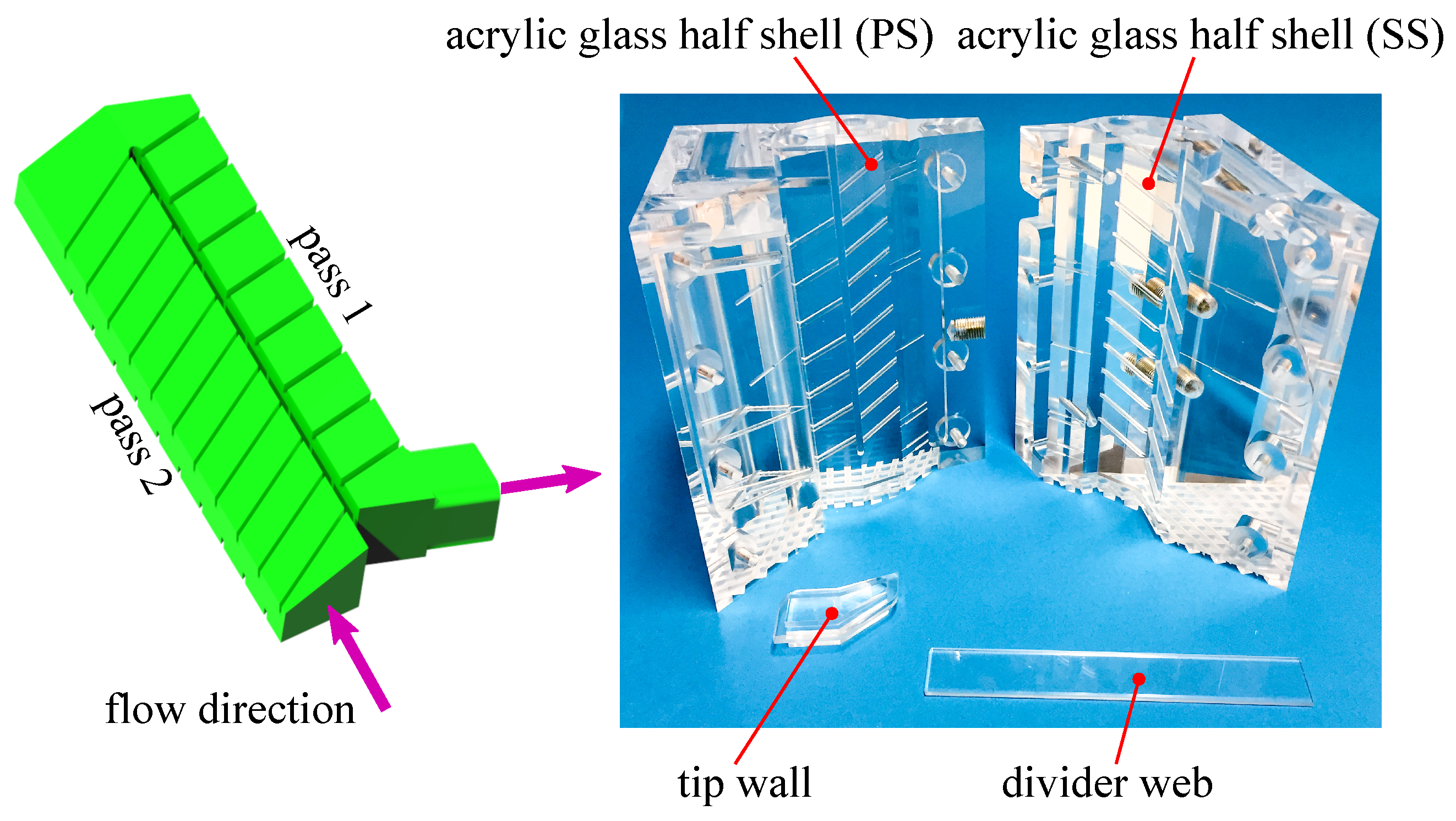
2. Test Model

The cooling-channel design is adapted from the non-rotating model discussed in [33]. Figure 1 illustrates the different components of the acrylic glass model (right) and the fluid domain (left).

The inlet passage (pass 1) features a trapezoidal cross-section and represents a leading-edge cooling channel with outward radial flow. We utilize its hydraulic diameter ($d_{\mathrm{h}}=$15 mm) as a reference for the calculation of dimensionless parameters when needed. A 180°-bend turns the flow radially inwards as it connects pass 1 to the outlet passage (pass 2). The latter is characterized by a rectangular cross-section. The suction-side (SS) and pressure-side (PS) surfaces present a staggered rib arrangement with rib angles between 60° and 65°.

The test model consists primarily of two acrylic glass (PMMA) half shells, a divider web, and a tip wall. The inner channel walls are coated with TLCs and black backing paint. Narrowband TLCs (type SPN100/G10C1W) from Hallcrest with an indication temperature of $T_{\mathrm{ind}}=11.1$ °C and a bandwidth of 1 $\mathrm{K}$ are used.

The model is equipped with 15 type-K thermocouples (TCs), which measure the fluid temperature histories along the channel. These TCs are wedged between the two half shells, with their tips directed to the geometric center of the respective cross-section. Three additional TCs are placed at various depths inside the acrylic glass block to monitor the temperature distribution within the model and guarantee the isothermal starting conditions.

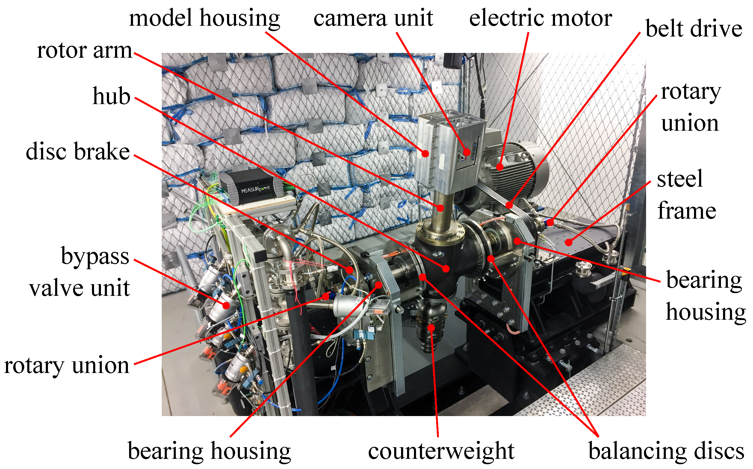
3. Experimental Setup

The rig design is described in detail in [12,14]. The rotor comprises a hollow main shaft, a hollow rotor arm, a model housing, and an adjustable counterweight on the opposing arm. Figure 2 provides an overview of the rig.

The test model is placed inside a model housing consisting of two aluminum half shells. The housing operates with air pressures up to 10 bar and is mounted at the end of the rotor arm, positioning the model at a mean radius of 750 mm. An electric motor with a frequency converter drives the rotor, reaching a maximum rotational speed of 900 rpm through a belt drive.

3.1. Rotor

Each end of the main rotor shaft is fitted with rotary unions to feed air into the rotating system. One rotary union is directly linked to the model and provides both tempering air (before the experiment) and test air (during the experiment). The second rotary union supplies precooled air to a separate secondary pipe system. This precooled air is utilized to lower the temperature of the test air supply pipes before the experiment. Thus, heat intake into the test air is minimized before it reaches the test model. This process ensures a suitable fluid temperature change required for the transient TLC experiment.

3.2. Rotating Camera Unit

A camera unit designed to capture the TLC color play during rotation is installed inside the model housing. The unit comprises a customized action camera, lighting and signal LEDs, an IR receiver, and batteries, all integrated into an aluminum plate [13]. The camera features 1080p full HD resolution at a frame rate of 30 fps and uses a 145° wide-angle lens, enabling close positioning relative to the model. To protect against operating pressures of up to 10 bar and to prevent video distortion, the camera lens and sensor are encapsulated and covered with protective glass. For homogeneous illumination of the model, four white LEDs with a color temperature of 6500 K are positioned in the corners. In order to synchronize the video with fluid temperature measurements, a single red LED is employed. The LED reflection on the acrylic glass model is visible in the video, and its switching is timed with the external data acquisition process. Two camera units are used to simultaneously capture the suction and pressure sides of the model.

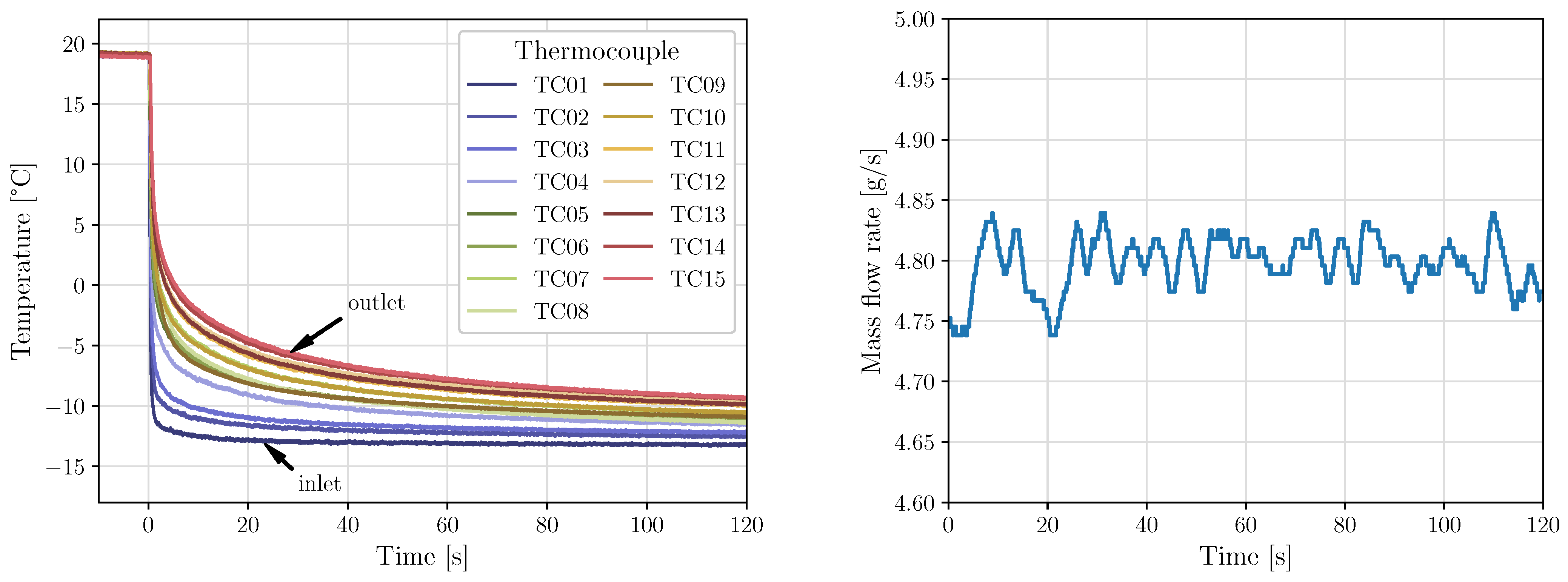
3.3. Fluid Temperature Change

The fluid temperature change is achieved using a bypass valve unit that controls the air supply to the model. In the tempering phase, tempering air is directed through the rotor passage. This air flow can be at ambient temperature or slightly heated and fulfills three functions. First, it establishes the isothermal starting temperature for the acrylic glass model. Secondly, it prevents cold air from the precooled central pipes of the rotor arm from entering the model during the rotor start-up process. This is achieved by reversing the flow direction compared with the experiment phase (see Figure 3). Thirdly, it sets a suitable pressure level to prevent a pressure jump at the beginning of the experiment, when the cold test air is switched to the rotor passage (experiment phase). To achieve extremely low temperatures (as low as −100 °C) for the precooled air and test air, a heat exchanger operated with liquid nitrogen is employed.

At the left-hand side of Figure 4, a typical fluid temperature change is depicted for an experiment conducted with a mass flow rate of $4.8$ $\mathrm{g}$/$\mathrm{s}$ ($Re\approx$ 15,000). At the model inlet, the fluid temperature quickly drops below the TLC indication temperature. As the test air warms up while traveling through the channel, the temperature change is correspondingly delayed further down the path. The resulting history of the mass flow rate is presented at the right-hand side of Figure 4.

3.4. Wall Temperature Change

TLCs serve as surface temperature sensors to determine the cooling rate of the channel walls after the sudden change in fluid temperature. By analyzing the fluid temperatures and the measured TLC indication times, which provide the surface temperature at the time of indication (i.e., the calibrated TLC indication temperature), heat transfer coefficients can be calculated.

The evaluation process is based on the solution of Fourier’s transient heat conduction equation considering the following boundary conditions: 1D heat conduction, an isothermal model start temperature, and a semi-infinite wall assumption. The applicability of the last two conditions was verified utilizing a preliminary test model equipped with multiple TCs positioned at varying depths inside the acrylic glass wall.

4. Experimental Data Acquisition and Synchronization

The synchronization signal, which marks the start of the experiment, is generated using a counter/timer module. In addition, an IR signal is sent to the camera unit to turn off the sync-LED, creating a temporal reference point in the video footage. With this, the synchronization of the different data needed for the heat transfer evaluation is achieved. The counter/timer module also manages the control signals for the valve unit, enabling the switch from the tempering state to the experimental state. The six valves are equipped with inductive sensors and can be individually preprogrammed with delay times, allowing for optimization of the switching procedure concerning the pressure and mass flow rate.

For data transmission, the telemetry system sends digitized 16-bit signals of temperature and pressure data from the model to the stationary receiver unit, which logs the data at a rate of 100 samples/$\mathrm{s}$.

5. Experimental Data Analysis

The transient TLC technique revolves around the measurement of the TLC indication times following an induced fluid temperature step change. A comprehensive explanation of this technique is provided in [34,35,36].

To prepare the video footage for evaluation using in-house code ProTeIn a few processing steps are necessary. First, the video is cut to synchronize the start of the footage with the onset of the fluid temperature drop recorded by the TCs at the channel inlet. Secondly, the fish-eye distortion caused by the wide-angle lens is corrected as described in [13]. Last, the video is cropped to focus only on the relevant heat transfer surface.

The first analysis steps in ProTeIn involve wavelet-based filtering and adaptive normalization, as outlined in [37]. Then, the time at which the intensity of the green channel reaches its maximum is determined for each pixel. This instant corresponds to the point in time when the surface reaches the TLC indication temperature. This temperature is determined beforehand through a stationary calibration procedure as described in [38].

The fluid temperature history for each pixel is computed using the CFD-supported approach outlined in [16]. The method relies upon the calculation of mass flow-averaged bulk temperatures in the numerical computation so as to derive a dimensionless temperature profile, which is then applied to the experiment. Through this, we obtain a time-dependent temperature distribution while maintaining the time behavior of the TLC experiment. By this means, issues regarding existing uncertainties in thermocouple positioning or temperature measurement at sensitive locations with strong temperature gradients, such as the bend region, are avoided. Heat transfer coefficients are subsequently calculated using the transient, one-dimensional Fourier heat conduction equation for a semi-infinite wall with a convective boundary condition.

To approximate the actual fluid temperature history, the Duhamel superposition principle [39,40] is utilized, representing the fluid temperature as a series of small, discrete temperature steps ($\Delta T_{\mathrm{f}(j,j-1)}$). This series accounts for the transient behavior of the fluid temperature following the induced temperature step change.

$$\begin{array}{c}{T}_{\mathrm{w}}-T_0=\sum _{j=1}^N\left[1-\exp \left({\beta }^2\right)\mathrm{erfc}\left(\beta \right)\right]\Delta T_{\mathrm{f}\left(j,j-1\right)}\hfill \\ \hfill \mathrm{with}\beta =h\sqrt{{\displaystyle \frac{t_{\mathrm{ind}}-{\tau }_j}{{\rho }_{\mathrm{w}}{c}_{\mathrm{P},\mathrm{w}}{k}_{\mathrm{w}}}}}.\end{array}$$

(1)

In the provided equation, $T_{\mathrm{w}}=T_{\mathrm{ind}}$ represents the wall temperature at the time of indication ($t_{\mathrm{ind}}$); $T_0$ denotes the initial model temperature; ${\tau }_j$ is a discrete point in time during the fluid temperature measurement; and ${\rho }_{\mathrm{w}}$, $c_{\mathrm{P},\mathrm{w}}$, and $k_{\mathrm{w}}$ are the physical properties of acrylic glass (density, heat capacity at constant pressure, and heat conductivity, respectively). Equation (1) is solved at each pixel position iteratively through the application of Newton’s method. As a result, a two-dimensional map of the heat transfer coefficient is obtained.

An estimation of the experimental uncertainty is presented in Appendix A.

6. Dimensionless Quantities

In the present investigation, test cases are classified in terms of Reynolds number ($Re$) and rotation number ($Ro$).

The Reynolds number is calculated from the measured mass flow rate, the channel geometry, and the dynamic viscosity, which is determined at the channel entry (TC0102).

$$Re={\displaystyle \frac{\rho u{d}_{\mathrm{h}}}{\mu }}={\displaystyle \frac{\dot{m}{d}_{\mathrm{h}}}{A\mu }}$$

(2)

The rotation number represents the dimensionless form of the rotational speed and is calculated from the latter, the hydraulic diameter, and the flow velocity at the channel inlet, which is derived from pressure and temperature measurements. These are conducted by means of an absolute pressure sensor and the thermocouple pair (TC0102), respectively.

$$Ro={\displaystyle \frac{\mathrm{\Omega }{d}_{\mathrm{h}}}{u}}$$

(3)

Besides Reynolds and rotation number similarity, the buoyancy number needs to be taken into account for rotating experiments, where centrifugal forces become significant and influence heat transfer. In our definition of $Bo$, the density ratio is expressed as a temperature ratio, where the temperature difference between the start-wall temperature of the model ($T_{\mathrm{w}}=T_{\mathrm{w}}(t=0)$) and the fluid temperature is considered. Furthermore, the ratio between mean model radius and hydraulic diameter is used.

$$Bo={\displaystyle \frac{\Delta \rho }{\rho }}R{o}^2{\displaystyle \frac{R}{d_{\mathrm{h}}}}=\left({\displaystyle \frac{T_{\mathrm{w}}-T_{\mathrm{f}}}{T_{\mathrm{w}}}}\right)R{o}^2{\displaystyle \frac{\overline{R}}{d_{\mathrm{h}}}}$$

(4)

The actual set of dimensionless parameters ($Re$, $Ro$, and $Bo$) of the present investigation is summarized in Appendix B.

Heat transfer rates are presented in their dimensionless form through the Nusselt number ($Nu$). This is calculated from the heat transfer coefficient, the hydraulic diameter, and the thermal conductivity of the fluid. The latter is averaged from the start of the experiment until the TLC indication time is reached.

$$Nu={\displaystyle \frac{h{d}_{\mathrm{h}}}{k_{\mathrm{f}}}}$$

(5)

7. Numerical Setup

The numerical methodology is based upon steady-state RANS simulations and is implemented in commercial CFD software package ANSYS CFX 21.1. In past investigations, this scheme proved to be accurate enough to correctly predict the local heat transfer characteristics in rotating cooling channels [16,17,30]. The RANS equations are solved in the enthalpy form with the k-$\omega$ SST turbulence model. We also introduce curvature correction and reattachment modification options, which are available in ANSYS CFX and were validated against experimental data in previous studies in a similar cooling channel geometry under rotating conditions [28].

Air is modeled as an ideal gas in order to take compressibility effects into consideration. Viscosity and thermal conductivity are temperature-dependent and are, therefore, determined by means of Sutherlands’s equations [41]. Rotation leads to Coriolis and centrifugal buoyancy forces, which are modeled as additional sources of momentum in the RANS equations [42].

All simulations considered in the present study achieved maximum residuals below $5\times {10}^{-3}$ in the momentum and energy equations. Furthermore, quantities that describe the flow field, such as pressure, velocity, and temperature, were locally monitored along the flow path in order to ensure the stability of the results.

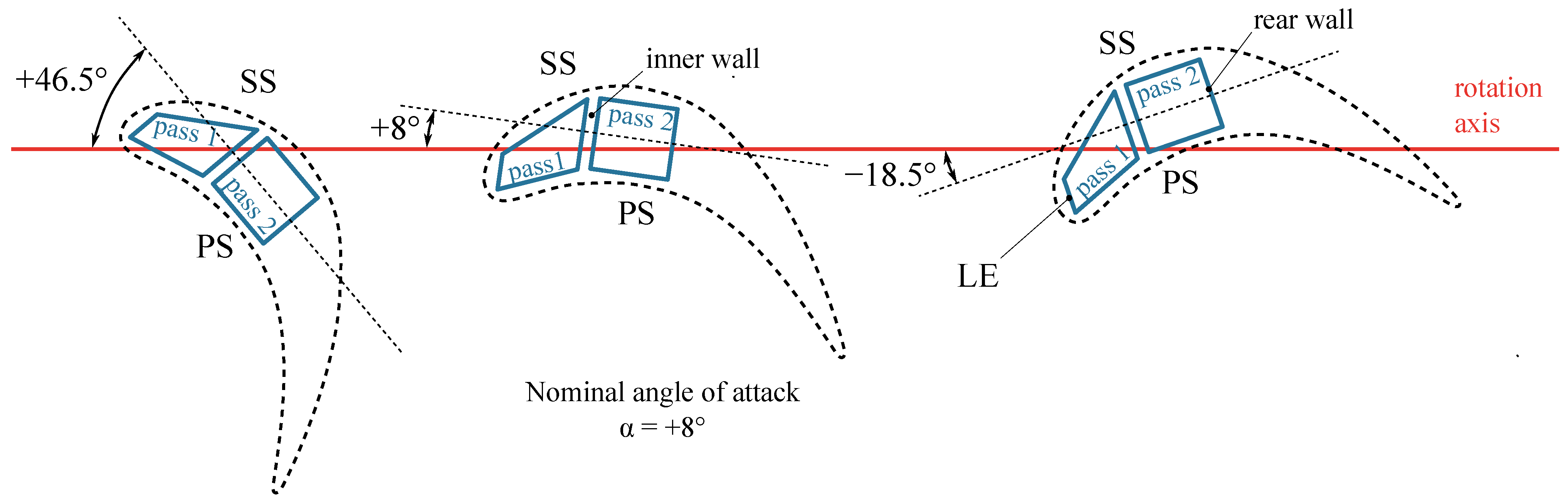
7.1. Angles of Attack

The internal cooling channel was investigated at different orientation angles or angles of attack, as represented in Figure 5, with the intention of providing a basis for validation against experiments. Through this, the prediction accuracy of the rotational direction and its magnitude can be examined. The choice of the three angles was based on the channel orientation at characteristic spanwise positions (hub, midspan, and tip) for twisted turbine blades. The nominal angle of attack ($\alpha =+8^{°}$) is taken as the reference value, corresponding to the midspan of the blade.

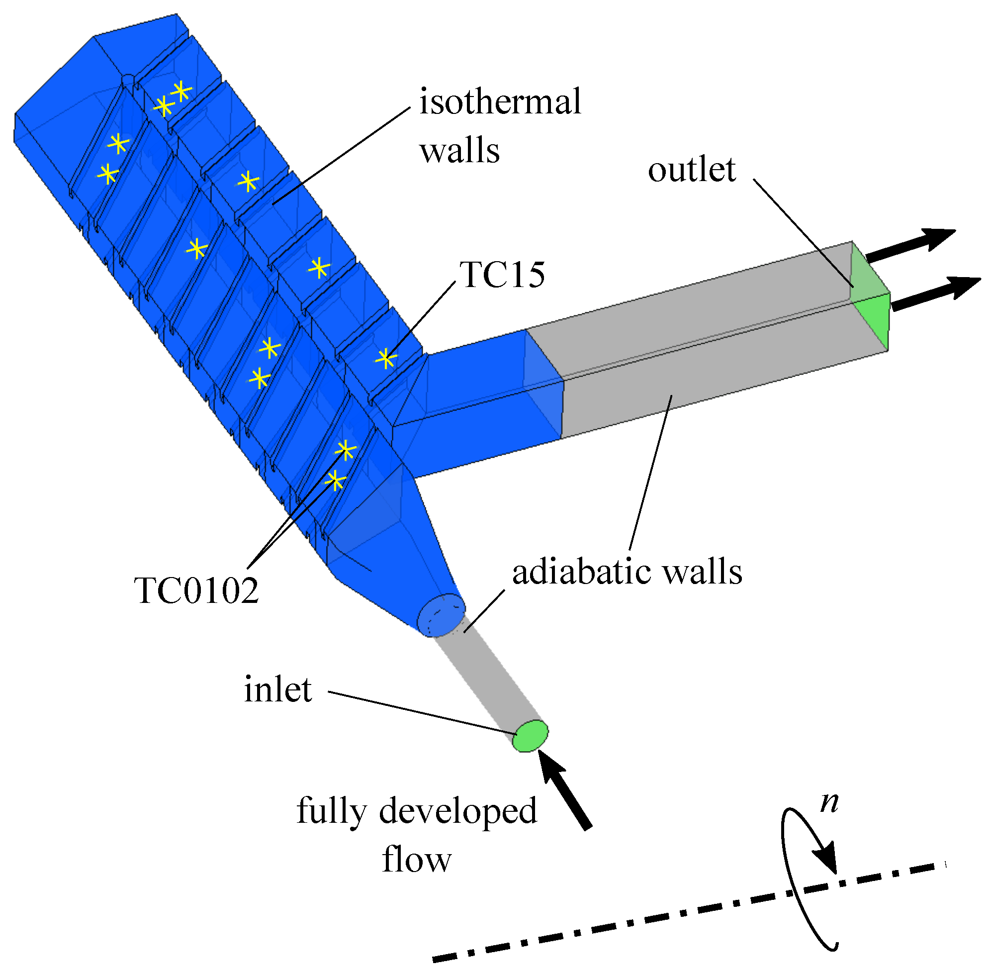
7.2. Boundary Conditions

Figure 6 schematically shows the cooling channel with the applied boundary conditions as well as the experimental temperature measurement locations through TCs (yellow crosses). Inflow conditions (velocity, temperature, turbulent kinetic energy, and turbulent length scale) are derived from a preceding calculation for a rotating pipe flow in order to obtain flow characteristics similar to those observed in the experiment (skewed, fully developed turbulent flow). The pipe flow represents the air supply from the rotor shaft to the test subject and was modeled with adiabatic walls. Considering this preceding computation for the pipe flow, the inlet temperature corresponds to the time-averaged fluid temperature for the duration of the TLC experiment measured with the thermocouple pair (TC0102). Sensitivity to the inlet temperature within a realistic frame (temperatures measured during the TLC experiment) proved to have a negligible impact on the heat transfer coefficient, although not demonstrated here. For the present investigation, the inlet temperature varied between −15.5 °C and −19.7 °C.

Wall temperature, including ribs, is held constant and equals the start temperature of the plexiglas model in the TLC experiment. For the investigated cases, it ranged between 18.9 °C and 22.3 °C. Furthermore, the no-slip boundary condition was applied.

Inflow and outflow sections to the channel are modeled as adiabatic. Moreover, the outflow is extended in order to capture any existing recirculation areas downstream of the 90°-turn.

A constant pressure boundary condition was applied to the outlet of the channel and was held constant at $p_{\mathrm{out}}=6\mathrm{bar}$ for all investigated cases. It was estimated as an average value of the existing pressures during the experiment.

Considering the rotating cases, the rotational speed from the experiment (n) was applied for the whole numerical domain.

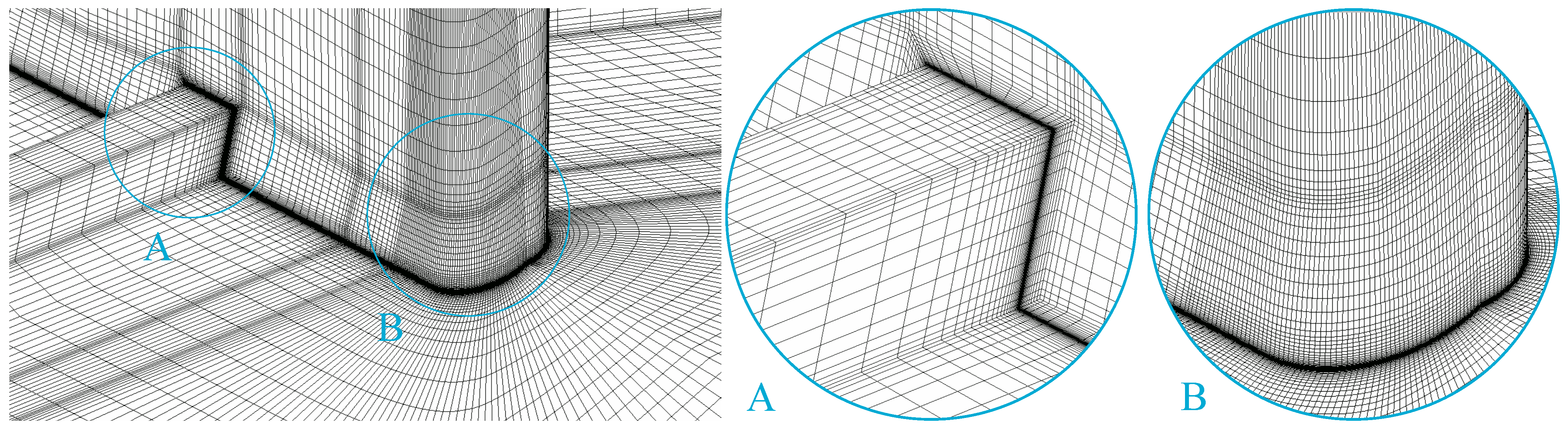
7.3. Computational Grid

A multi-block structured approach was undertaken for the computational mesh generation in the commercial software package ANSYS ICEM 17.1. The meshing strategy consisted of the separate generation of unique channel segments, which were ultimately concatenated to create the investigated cooling channel. By means of this approach, better control of the dimensionless wall distance and the mesh quality parameters (grid angle, aspect ratio, and volume change, amongst others) could be achieved. These were within the recommended limits defined in the ANSYS ICEM CFD User’s Manual [43]. Considering the interfaces between the different channel segments, special attention was devoted to the alignment of the nodes from both sides, which helps to avoid unnecessary flux interpolation of the calculated variables. This would be detrimental to the CFD simulation as it would induce an additional source of numerical error.

The computational grid consisted of a total of 11.7 million nodes for the cooling channel and $9\times {10}^5$ nodes for the funnel geometry. Near-wall regions were refined so as to achieve a dimensionless wall distance of $y_1^{+}\approx 1$, which is imperative for accurate heat transfer calculations. Some mesh features can be observed in Figure 7.

8. Numerical Heat Transfer Evaluation

With regard to the numerical simulation, heat transfer rates between the coolant and the channel walls are calculated locally by means of Newton’s Law of Cooling [44] and presented as Nusselt numbers (Nu) as follows:

$$Nu={\displaystyle \frac{h{d}_{\mathrm{h}}}{k\left(T_{\mathrm{ref}}\right)}}={\displaystyle \frac{\frac{{\dot{q}}_{\mathrm{w}}}{(T_{\mathrm{w}}-T_{\mathrm{ref}})}{d}_{\mathrm{h}}}{k\left(T_{\mathrm{ref}}\right)}}$$

(6)

The selection of the reference temperature ($T_{\mathrm{ref}}$) may have an immense impact on the heat transfer coefficient and is far from trivial. A typical issue that arises in case a unique reference temperature is chosen for the whole channel, e.g., at the channel inlet, is that the temperature increase along the flow path is not taken into consideration, leading to heat transfer underestimation at those regions farther downstream than the channel inlet. In previous investigations, thorough thought and effort were devoted to compare different reference temperatures for the heat transfer evaluation, including centerline temperatures and temperatures evaluated at specific positions (i.e., TC locations in the experiment), among others [30]. A valid definition was found through calculation of a unique bulk temperature for each PS and SS segment evaluated at the different cross-sections in the cooling channel. By this means, the total energy balance of the flow is taken into account at each cross-section.

In the present investigation, the latter strategy is utilized, thereby defining a unique bulk temperature for each PS and SS segment in the channel as a mass flow-averaged quantity. Furthermore, the thermal conductivity of the air is evaluated for these temperatures, as shown in Equation (6).

9. Results and Discussion

In order to account for possible deviations in the Reynolds number between rotating and non-rotating cases, as well as between experimental and numerical results, the local Nusselt number is normalized with the Nusselt number from the Dittus–Boelter/McAdams correlation for fully developed turbulent channel flow [45], defined as

$$N{u}_0=0.023R{e}_{\mathrm{in}}^{0.8}P{r}_{\mathrm{in}}^{0.4}$$

(7)

This Nusselt number ($N{u}_0$) is unique for every test case, in contrast to the pixel-wise determined $Nu$. The exponent ($n=0.4$) for the Prandtl number ($Pr$) can be utilized as long as the coolant is colder than the channel walls, which is certainly the prevailing condition for all test cases considered here. Both $R{e}_{\mathrm{in}}$ and $P{r}_{\mathrm{in}}$ are calculated considering the measured temperatures at the thermocouple position TC0102 (averaged temperature of TC01 and TC02; see Figure 6) located at the channel inlet. The validity range for this correlation is $Re>{10}^4$ and is fulfilled throughout this investigation. Through this normalization procedure, a measure for heat transfer enhancement relative to the smooth channel is obtained.

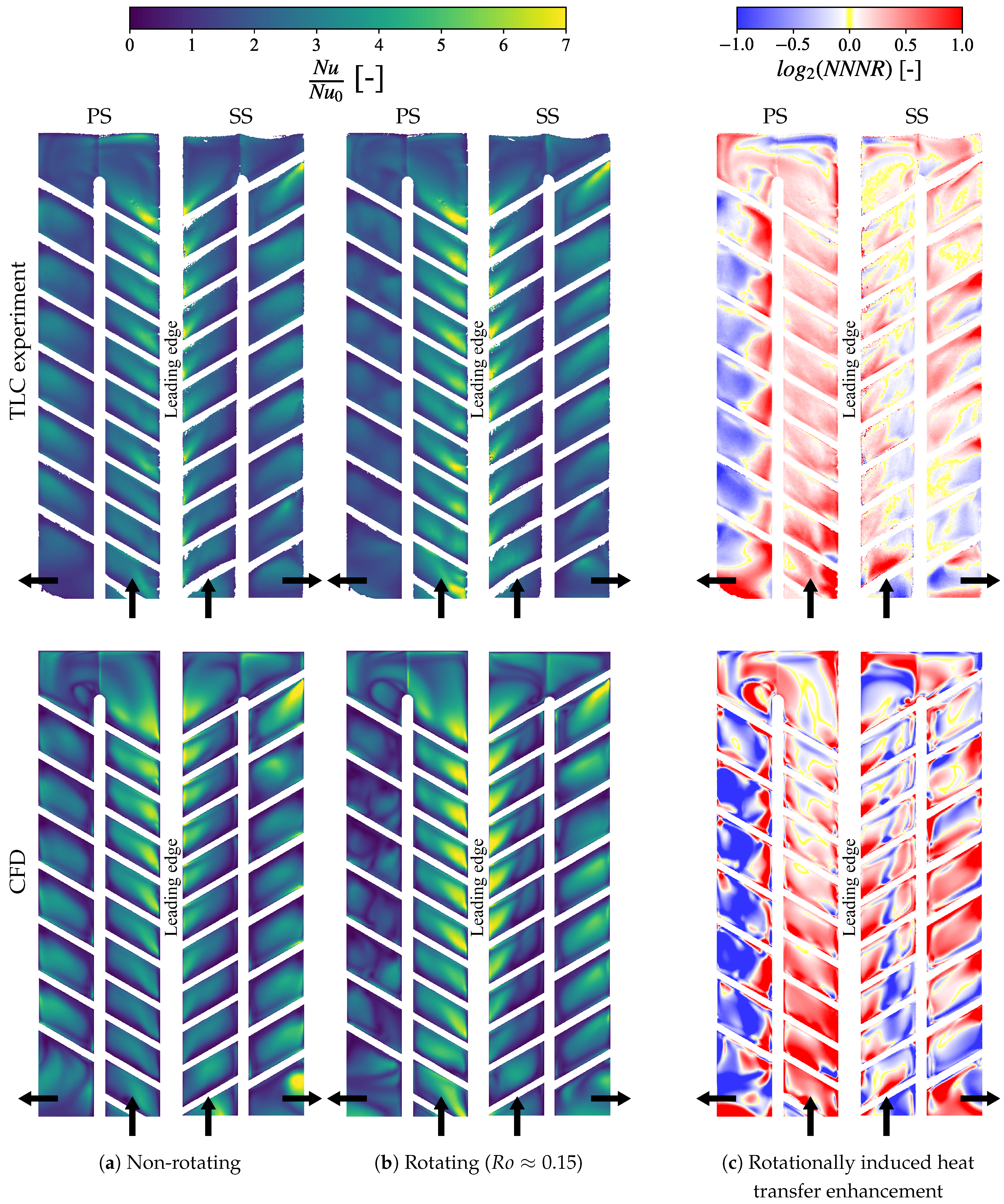
9.1. General Heat Transfer Characteristics

In Figure 8b, exemplary local heat transfer rates at the pressure side (PS) and suction side (SS) are depicted for the test case $Ro\approx 0.15$ with a nominal angle of attack ($\alpha =+8^{°}$) in the form of $Nu/N{u}_0$ contour plots. Its corresponding non-rotating case is presented in Figure 8a. The inner wall separates pass 1 and pass 2 (see Figure 5), and the 60°-angled ribs are masked out. At both the channel inlet and outlet, black arrows highlight the flow direction. Experimental TLC results are displayed at the top of the figure, and, for the sake of verification, CFD results are provided at the bottom.

The experimental non-rotating case displayed at the top of Figure 8a features the classical heat transfer pattern of a ribbed channel flow. In the radially outward flow of pass 1, angled ribs detach the air from near-wall regions and appear to drive it towards the leading edge (LE), as suggested by the heat transfer distributions from PS and SS. The flow then reattaches and heat transfer augmentation is expected in one of the most thermally stressed parts of the turbine blade, i.e., the leading edge. In the surrounding areas of the leading edge, both at PS and SS, the flow downstream of the ribs obliquely impinges the channel walls, thereby increasing heat transfer rates (yellow areas) by a factor as high as $Nu/N{u}_0\approx 7$ relative to the smooth channel. Downstream of the bend region, directly after the first rib, a spike in heat transfer at the SS can be observed. At the 180° bend, the channel shape changes from trapezoidal in pass 1 to rectangular in pass 2, with an increase in the cross-sectional area. The complex secondary flow structure induced by the bend appears to redirect the air towards the SS, resulting in this remarkable streak of increased heat transfer. Considering further downstream regions in pass 2, a similar pattern between PS and SS is observed, owing to the passage symmetry. All the above-mentioned comments are applicable to the CFD data presented at the bottom of Figure 8a, resulting in a qualitatively satisfactory agreement between the TLC experiment and CFD.

A first glance at the experimental results presented at the top of Figure 8b suggests that the rotational effect is beneficial, especially for PS pass 1, in terms of heat transfer augmentation (i.e., more heat pickup) compared with the non-rotating case. As regards pass 1, rotation leads to a Coriolis force directly proportional to the rotational speed with the direction of the vector of rotation, which drives the cold air from the suction side walls towards the pressure side walls (see Figure 5) and returns to the SS, upwashing the side walls. At PS pass 1, thinner boundary layers with increased turbulence levels are responsible for the enhancement of heat transfer. The Coriolis force changes its vector sign for radially inward flow so that heat transfer is noticeably reduced for PS pass 2 and increased for SS pass 2 as a result of rotation. The skewness of the velocity profiles under rotating and non-rotating conditions were investigated experimentally by Liou et al. [46]. The authors reported that the highest streamwise near-wall velocities in the second passage occurred at the SS, confirming the results presented here in the form of heat transfer distributions. Moreover, not only the overall heat transfer level, but also the local heat transfer shape, is prone to change due to the rotational effect, as can be observed in PS pass 2. In this region, distinctive pairs of structures with enhanced heat transfer appear in each rib segment, which were not present in the non-rotating case. These structures are also visible in the CFD contour plots. Further insights into the experimental–numerical agreement are provided in Section 9.2.

A means to isolate and directly assess the influence of rotation on heat transfer is through the calculation of the normalized Nusselt number ratio (NNNR) of the rotating case relative to its corresponding non-rotating case.

$$\mathit{NNNR}(x,y)={\displaystyle \frac{{\left(\frac{\mathit{Nu}(x,y)}{{\mathit{Nu}}_0}\right)}_{\mathrm{ROT}}}{{\left(\frac{\mathit{Nu}(x,y)}{{\mathit{Nu}}_0}\right)}_{\mathrm{STAT}}}}$$

(8)

Any possible systematic measurement errors can be reduced through the formation of normalized Nusselt number ratios, since these errors should affect the absolute Nusselt number values of rotating and non-rotating cases by the same amount. Nevertheless, direct NNNR data representation through the above-mentioned approach could give rise to misleading interpretations if NNNR data were directly plotted, e.g., as contour plots. Consider two pixel positions in a contour plot as an example; in one of them, the term ${\left.Nu/N{u}_0\right|}_{\mathrm{ROT}}$ is twice as high, and in the other one, it is half as high as in their respective pixels in the non-rotating case, i.e., ${\left.Nu/N{u}_0\right|}_{\mathrm{STAT}}$, resulting in $\mathit{NNNR}=2$ and $\mathit{NNNR}=0.5$, respectively. By applying a divergent color legend from 0 to 2 centered in $\mathit{NNNR}=1$ (i.e., ${\left.Nu/N{u}_0\right|}_{\mathrm{ROT}}={\left.Nu/N{u}_0\right|}_{\mathrm{STAT}}$), heat transfer increase and decrease due to rotation can be disclosed, yet the level to which it is increased/decreased could be misinterpreted by the reader. Doubling of heat transfer rates (×2) would be visually overestimated, and a 50% decrease (×0.5) would be underestimated. In order to avoid bias in favor of heat transfer enhancement, the authors opted for a data representation in which heat transfer enhancement and reduction factors are equally weighted in the contour plot color bar. Through calculation of the logarithm with base 2 of NNNR data, this issue can be tackled. Its usage is, therefore, highly recommended by the authors for the assessment of local rotational heat transfer effects and will be utilized in the following.

The results presented in Figure 8a,b are shown in Figure 8c as $lo{g}_2\left(\mathit{NNNR}\right)$ contour plots. Red areas indicate an increase in heat transfer, blue areas indicate a decrease in heat transfer, and yellow areas, i.e., $lo{g}_2\left(\mathit{NNNR}\right)\approx 0\to \mathit{NNNR}\approx 1$, remain unchanged or minimally affected by rotation. As can be observed, rotation mainly yields a heat transfer increase in PS pass 1, where the enhancement can reach a factor of up to two $lo{g}_2\left(\mathit{NNNR}\right)\approx 1\to \mathit{NNNR}\approx 2$. Contrarily, rotationally induced heat transfer can also be detrimental, as in some areas of PS pass 2 and the SS. More details on the impact of rotation on heat transfer are presented in the following sections.

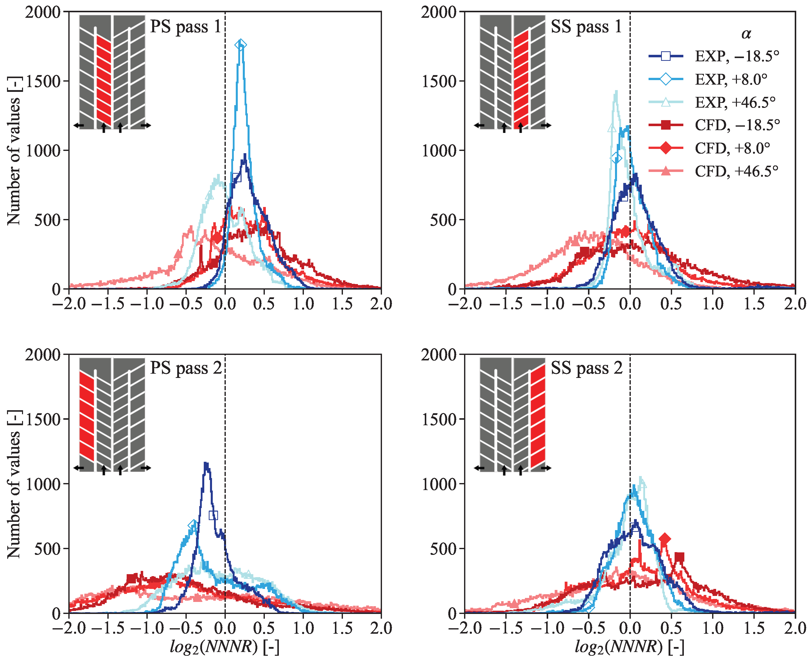
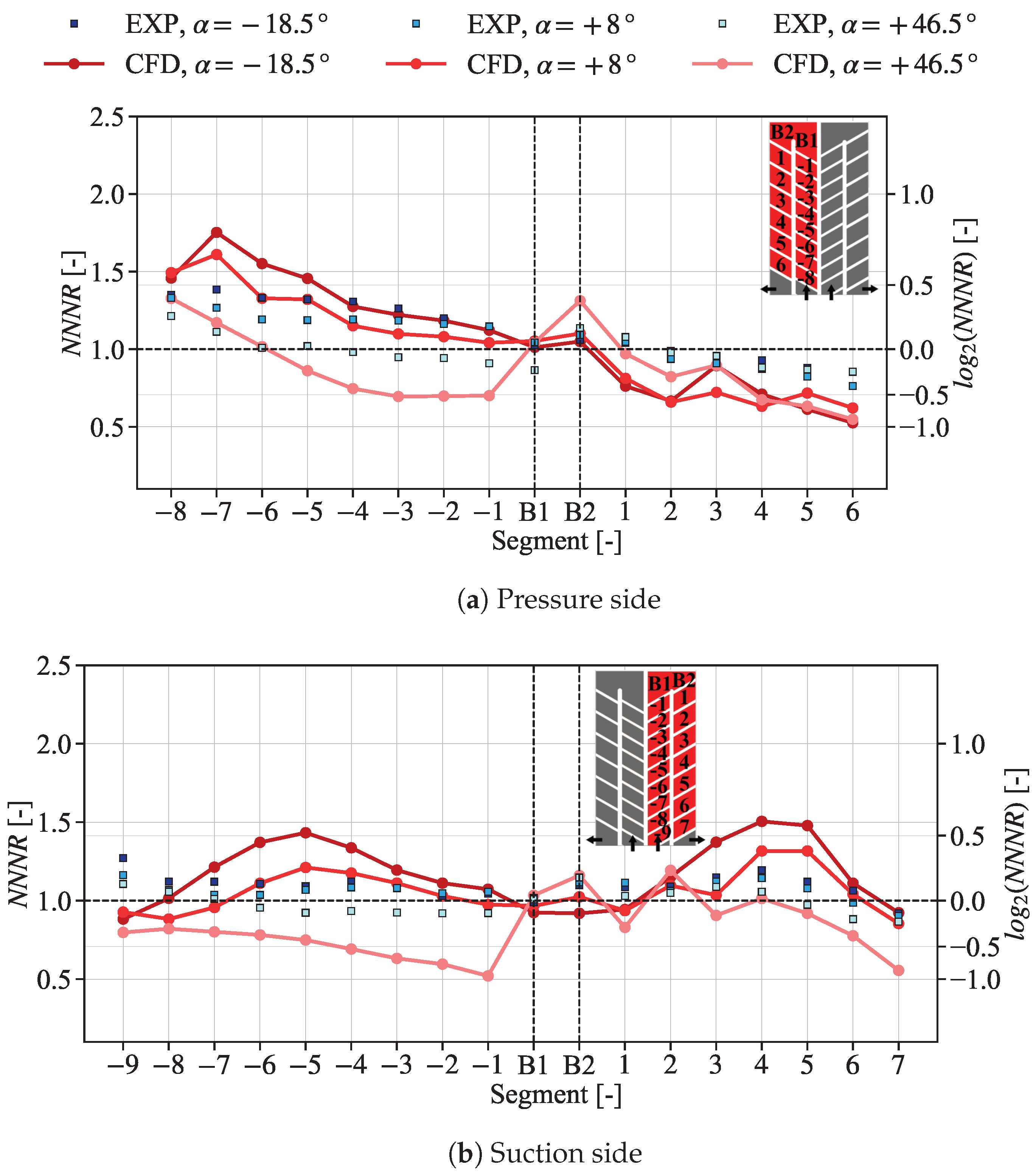
9.2. Numerical Validation at Different Angles of Attack

As introduced in Section 7.1, the cooling channel was investigated at three different angles of attack ($\alpha =+{46.5}^{°};+8^{°};-{18.5}^{°}$) so as to provide a validation basis for the numerical model. A change in the angle of attack under unaltered rotating conditions triggers a different direction of the Coriolis force, thereby altering the secondary flow field. This, in turn, modifies the local heat transfer footprint. A well validated numerical model under different angles of attack is not only able to support the experimental approach but can also be helpful as a design baseline for more complex twisted turbine blades. In the following, we discuss the rotationally induced heat transfer characteristics for a rotation number of $Ro\approx 0.15$ with the help of contour plots of the normalized Nusselt number ratios for the TLC experiment and CFD presented at the top and the bottom of Figure 9, respectively. First, the discussion focuses on the nominal angle of attack. Then, the other two angles are considered.

The nominal angle of attack ($\alpha =+8^{°}$) features high rotationally induced heat transfer rates for PS pass 1, as expected based on the governing direction of the Coriolis force. Here, NNNR appears to be highest in the upstream rib segments, i.e., close to the channel inlet, and tends to gradually decrease further downstream until the bend region is reached, maintaining generally positive heat transfer rates ($lo{g}_2\left(\mathit{NNNR}\right)>0\to \mathit{NNNR}>1$). In the most downstream part of each rib segment, however, local heat transfer rates are reduced (see A1 in Figure 9b) so that $lo{g}_2\left(\mathit{NNNR}\right)\approx 0$ or locally drop to negative values. The numerical results forecast higher heat transfer rates in the upstream rib segments and lower heat transfer rates in rib segments closer to the bend, in agreement with the experiment. Overall, the CFD prediction delivers higher gradients of NNNR than the experiment, i.e., brighter blue/red areas and thinner transitions where $lo{g}_2\left(\mathit{NNNR}\right)\approx 0$, which can be partly justified by the assumption of one-dimensional heat conduction in the experimental analysis (Equation (1)). Although not demonstrated here, three-dimensional heat conduction effects become especially relevant for increasing indication times and for complex cooling channels and turbulator designs. The purpose of turbulators, such as ribs, is to enhance heat transfer by increasing the surface in contact with the cooling air and by inducing a secondary flow field which generates turbulent mixing. As a direct consequence, ribs naturally cool down faster than the adjacent surfaces, i.e., they necessarily absorb heat from neighboring regions during the transient TLC experiment. In other words, regions adjacent to ribs reach the indication temperature ($T_{\mathrm{ind}}$) sooner than they would without the existence of lateral heat conduction effects (i.e., three-dimensional heat conduction), thereby leading to an overestimation of the heat transfer coefficient. Contrarily, whenever sharp lateral gradients in the heat transfer coefficient distribution are present, regions where the heat transfer coefficient is intrinsically high are underestimated in favor of adjacent regions where the heat transfer coefficient is lower. As a result, the experimental method tends to produce a generally milder local heat transfer footprint (i.e., with softer gradients) than its numerical counterpart, as can be observed through comparison of the top and bottom plots of the local heat transfer rates from Figure 8a,b. Moreover, since rotation locally alters the secondary flow field, the sharp $Nu/N{u}_0$ gradients observed in the CFD contour plots in Figure 8 translate to sharp gradients in $lo{g}_2\left(\mathit{NNNR}\right)$.

PS pass 2 is characterized by a distinctive heat transfer pattern, which features a positive effect, i.e., $lo{g}_2\left(\mathit{NNNR}\right)>0$, on surfaces next to the inner wall (A2) and a negative effect, i.e., $lo{g}_2\left(\mathit{NNNR}\right)<0$, on the remaining areas (A3). A similar phenomenon can be discerned from SS pass 1, where regions adjacent to the leading edge generally achieve positive NNNR rates (A4) and are clearly divided from regions next to the inner wall (A5) with a dashed line. Considering the region A5, some discrepancies between experimental and numerical results arise. As for the TLC experiment, A5 extends until the end of the first passage, in contrast to the CFD results, where A5 is limited to a relatively small region of pass 1. In any case, the areas in which the CFD and experimental results show inconsistencies in predicting the correct sign of NNNR are comparably tiny. Additionally, it is worth mentioning the fact that the surfaces on the peripheries of the leading edge achieve higher heat transfer rates under rotation than without rotation. This is highly relevant, since the leading edge is certainly an area of the turbine blade exposed to the highest thermal stresses, and additional cooling through the rotational effect can be strongly beneficial.

The PS and SS bend region (A6) is an area of the cooling channel with relatively high complexity, where inconsistencies between the TLC experiment and CFD appear. Here, the cooling air turns 180° from the trapezoidal cross-section of pass 1 to the rectangular pass 2. The Dean-type vortices and the recirculation bubble downstream of the bend seem to exhibit a much milder footprint in the TLC experiment than in the CFD. Nevertheless, in disregard of some local effects, the numerical prediction is overall consistent with the experimental results. Further downstream, SS pass 2 alternates regions with heat transfer increase and heat transfer decrease due to rotation. Here, as in the previously considered areas of the cooling channel, the qualitatively good agreement between the CFD prediction and the experiment must be emphasized again.

The local heat transfer footprint for the channel orientation of $\alpha =-{18.5}^{°}$ presented in Figure 9c resembles that of the nominal angle of attack. In accordance with our expectations, its structure remains unaltered for the most part, since the orientation of the inner channel walls with respect to the rotation axis does not change dramatically. As for pass 1, the channel walls exhibit a negative orientation with respect to the rotation axis for both considered angles, as depicted in Figure 5. Contrarily, for pass 2, the orientation changes from slightly positive for $\alpha =+8^{°}$ to negative for $\alpha =-{18.5}^{°}$. The previously described regions (A1…A6), as well as the remarks regarding the experimental–numerical agreement, hold true for $\alpha =-{18.5}^{°}$.

The channel orientation of $\alpha =+{46.5}^{°}$ unveils major changes in the heat transfer structure with rotation, as can be observed from the contour plots in Figure 9a. Broad parts of pass 1, mainly next to the leading edge (A7), are negatively affected by the channel rotation, with $lo{g}_2\left(\mathit{NNNR}\right)<0\to \mathit{NNNR}<1$. As a consequence of the new direction of the governing Coriolis force, the cooling air is no longer directed towards the leading edge but towards the corner side between the PS and the inner wall. A further outcome of the prevailing Coriolis force direction is a spot with high heat transfer rates in the bend region (A8). Here, rotation causes the cooling air to impinge on the rear wall and on PS bend pass 2. For the other angles of attack this area is significantly less pronounced. PS and SS of pass 2 share a heat transfer structure similar to that for the other angles of attack (see, e.g., regions A2 and A3).

A useful data visualization to qualitatively assess the change in angle of attack is derived from Waidmann et al. [15] and involves the use of $lo{g}_2$ (NNNR) histograms. Considering the data presented in Figure 9, the channel regions PS pass 1, SS pass 1, PS pass 2, and SS pass 2 are evaluated individually in Figure 10. Only the rib segments highlighted in red in each subfigure are taken into account, which means that the truncated segments and the inlet and outlet are neglected. The experimental (EXP) and numerical (CFD) datasets are plotted with a bin width of 0.01. Furthermore, due to the differing resolution (number of values) between experimental and numerical results, the numerical datasets have been linearly interpolated to the experimental map, thereby ensuring the same number of values for both experimental and numerical datasets in each channel region.

As observed in PS pass 1 (top left-hand side of Figure 10), the highest heat transfer enhancement due to rotation is achieved with an angle of attack of $-{18.5}^{°}$, as shown in dark blue (TLC experiment) and dark red (CFD), with a peak in the value count around $lo{g}_2\left(\mathit{NNNR}\right)\approx 0.3$. Contrarily, an angle of $+{46.5}^{°}$ under rotation generally results in decreased heat transfer rates and is centered at $lo{g}_2\left(\mathit{NNNR}\right)\approx -0.1$. Moreover, the highest value for $+8^{°}$ is found at $lo{g}_2($NNNR$)\approx 0.25$. This peak can be easily recognized in the experimental data, in contrast to the numerical data sets, in which distributions are much flatter and any peak is smoothed out. This supports the observation noted previously regarding the higher NNNR gradients existing in the CFD. The histogram plot for SS pass 1 shown at the top right-hand side of Figure 10 presents a tendency similar to that of PS pass 1, with a shift towards lower NNNR levels for an angle of $+{46.5}^{°}$.

In regard to pass 2, changes in NNNR are not so obvious, i.e., do not follow a recognizable trend. Whereas the peak in the experimental values shown at $lo{g}_2($NNNR$)\approx -0.25$ in PS pass 2 for $-{18.5}^{°}$ is flattened out with an increasing angle of attack, marginal change is observed in the numerical results. The same applies to SS pass 2, where the numerical method generally forecasts smoother and broader distributions than its experimental counterpart, i.e., higher heat transfer over- and underestimation due to rotation.

Figure 9 and Figure 10 enable qualitative assessment of heat transfer augmentation/reduction due to rotation. For a quantitative analysis, however, another data reduction method is required. In Figure 11, the datasets from Figure 9 are segmentally averaged and plotted in two XY diagrams for PS (top) and SS (bottom), respectively. We supplement the diagrams with an NNNR axis in order to allow for direct comparison with published literature without the need to transform the $lo{g}_2\left(\mathit{NNNR}\right)$ data. As regards the PS, the highest heat transfer enhancement rates are found at the inlet region (segment $-7$) for $\alpha =-{18.5}^{°}$, with $lo{g}_2\left(\mathit{NNNR}\right)\approx 0.47\to \mathit{NNNR}\approx 1.38$ (TLC experiment) and $lo{g}_2\left(\mathit{NNNR}\right)\approx 0.81\to \mathit{NNNR}\approx 1.75$ (CFD), and decrease steadily in the streamwise direction until the outlet of the cooling channel is reached. As visualized through the contour plots in Figure 9b,c for the angles $+8^{°}$ and $-{18.5}^{°}$ respectively, heat transfer enhancement dominates clearly in pass 1. Furthermore, it is worth mentioning the quite similar heat transfer distribution for both angles noted in the qualitative assessment through histogram plots, which results in a slightly higher overall heat transfer rates for $\alpha =-{18.5}^{°}$. In contrast, $\alpha =+{46.5}^{°}$ features reduced heat transfer level in pass 1 as a result of rotation for the majority of the channel segments.

When it comes to the suction side of the cooling channel, segment-averaged data are presented in Figure 11b. The CFD forecasts a remarkable heat transfer reduction due to rotation in pass 1 for $\alpha =+{46.5}^{°}$. Further downstream, however, a better experimental–numerical agreement is observed.

As demonstrated through the assessment of the segment-averaged results, the sign of $lo{g}_2\left(\mathit{NNNR}\right)$ is correctly predicted by the numerical method for most of the segments at PS and SS, yet the level to which heat transfer increase and decrease occur shows relevant deviations between the TLC experiment and CFD. Possible reasons for these deviations are outlined as follows:

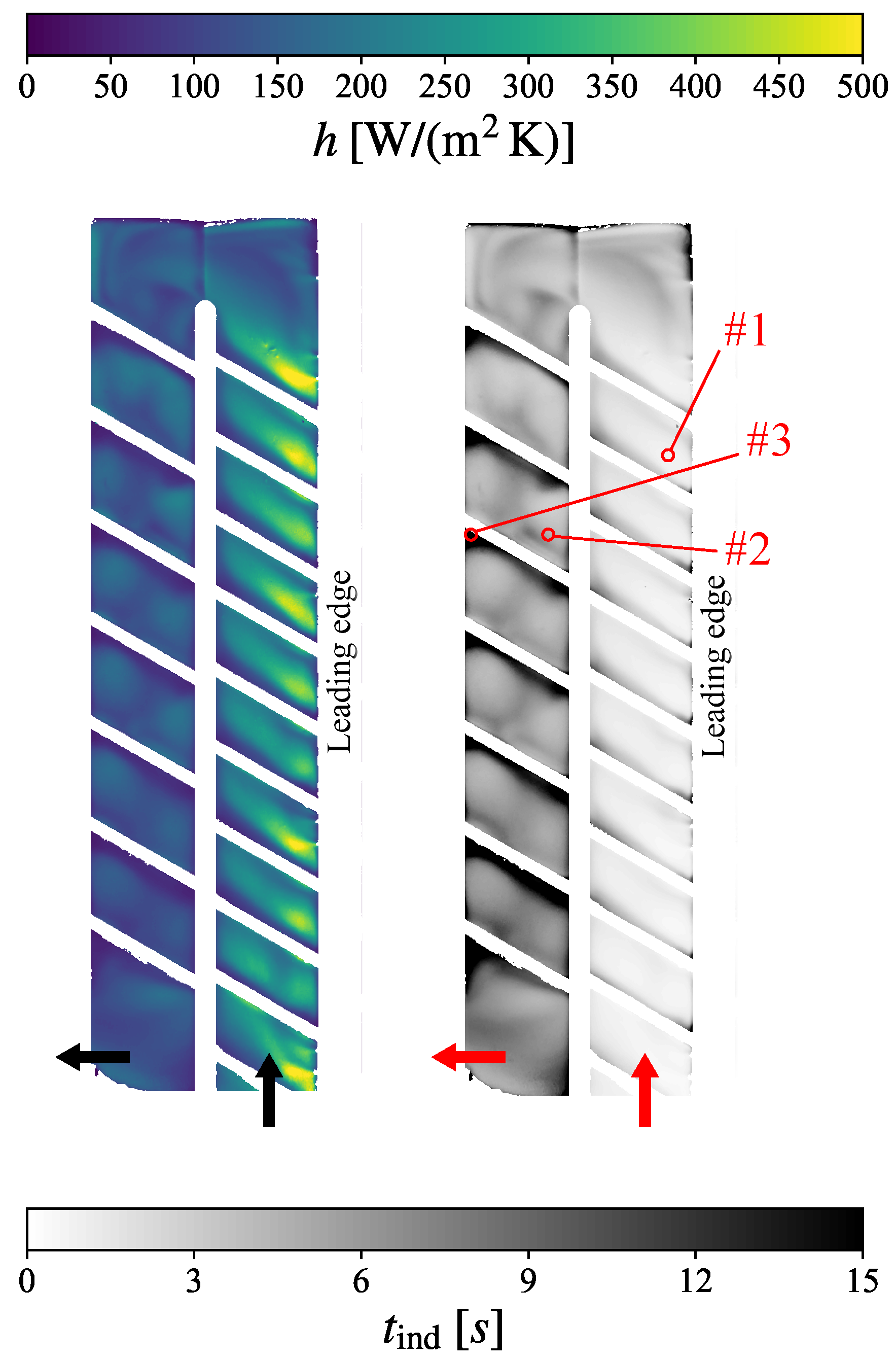
• Experimental uncertainty: In order to assess the uncertainty of a typical TLC experiment, a Monte Carlo analysis was performed on three different representative pixels, which is presented in Appendix A. Results disclosed local deviations up to 16.6% in the heat transfer coefficient (h) and up to 22.2% in the normalized Nusselt number ratio (NNNR).
• Lateral heat conduction effects present in the TLC experiment, as mentioned in the beginning of Section 9.2. The estimation of this experimental error is far from trivial, since there exist no simple analytical solutions for the transient three-dimensional heat conduction equation which can be applied here.
• Mismatch in the buoyancy number ($Bo$) between the transient TLC experiment and the steady-state numerical simulation. In order to fully address the effect of $Bo$ on the heat transfer rates, a computationally expensive transient conjugated CFD simulation would be required. On average, however, the time-averaged $Bo$ for the experiment and numerical simulation are well aligned, as reflected in

  Table A3. Actual dimensionless quantities for the investigated test cases.

  			TLC Experiment			CFD
  Parameter	Target Value	Angle:	+46.5°	+8°	−18.5°	+46.5°	+8°	−18.5°
  $Re$	15,000		14,915	14,910	14,821	14,832	14,890	14,913
  			14,881	15,106	14,836	14,843	15,098	14,891
  				14,964			14,967
  				14,634			14,612
  $Ro$	0		0	0	0	0	0	0
  	$0.15$		$0.149$	$0.152$	$0.148$	$0.149$	$0.152$	$0.150$
  	$0.30$			$0.305$			$0.303$
  	$0.50$			$0.499$			$0.492$
  $Bo$	0		0	0	0	0	0	0
  	$0.130$		$0.116$	$0.140$	$0.119$	$0.119$	$0.138$	$0.116$
  	$0.553$			$0.508$			$0.505$
  	$1.621$			$1.345$			$1.312$

  .
• Numerical modeling error and discretization error. The latter effect was quantified through a mesh independence study (not reported here) and resulted in uncertainties of up to 6% for the PS and 3% for the SS.

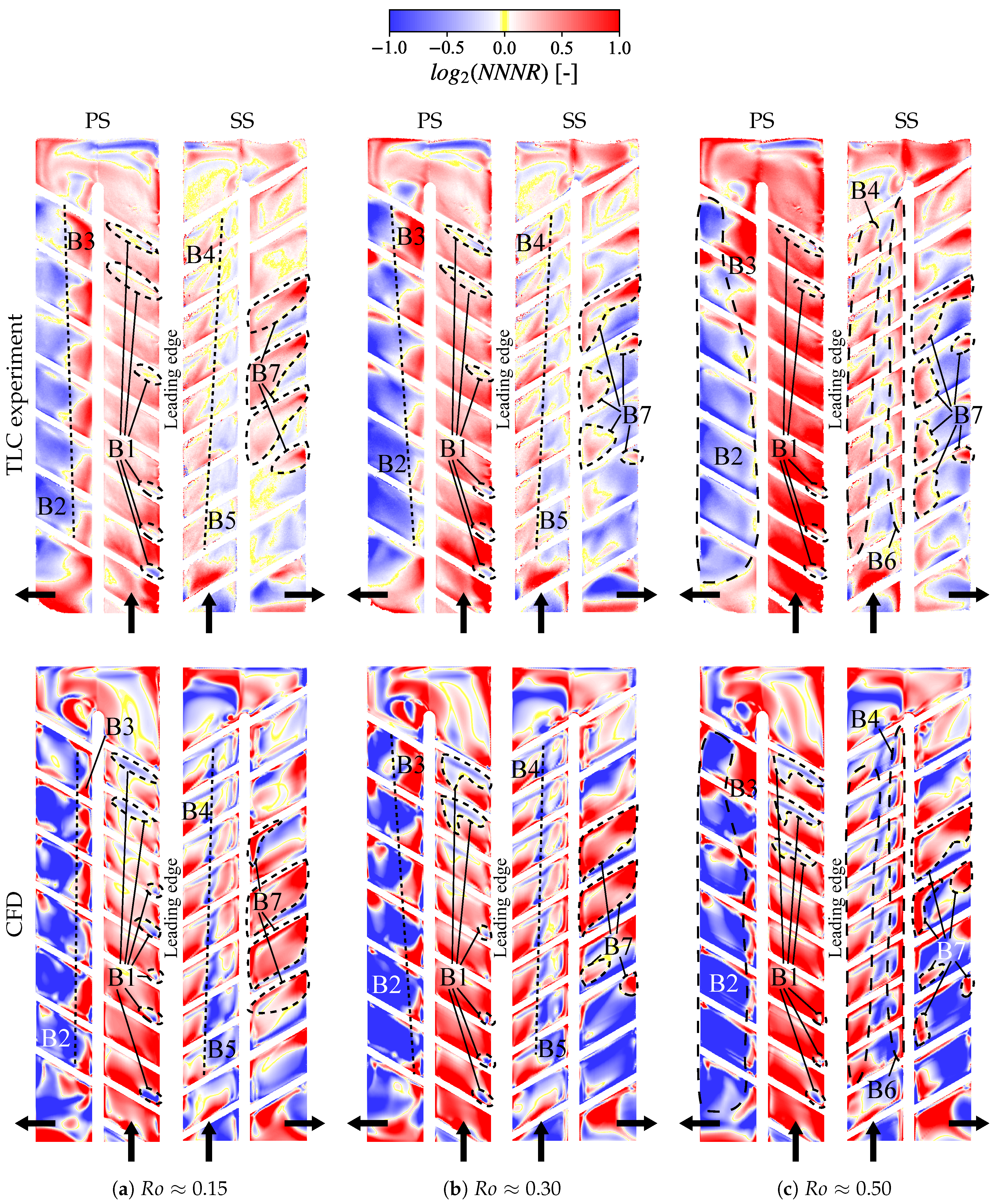
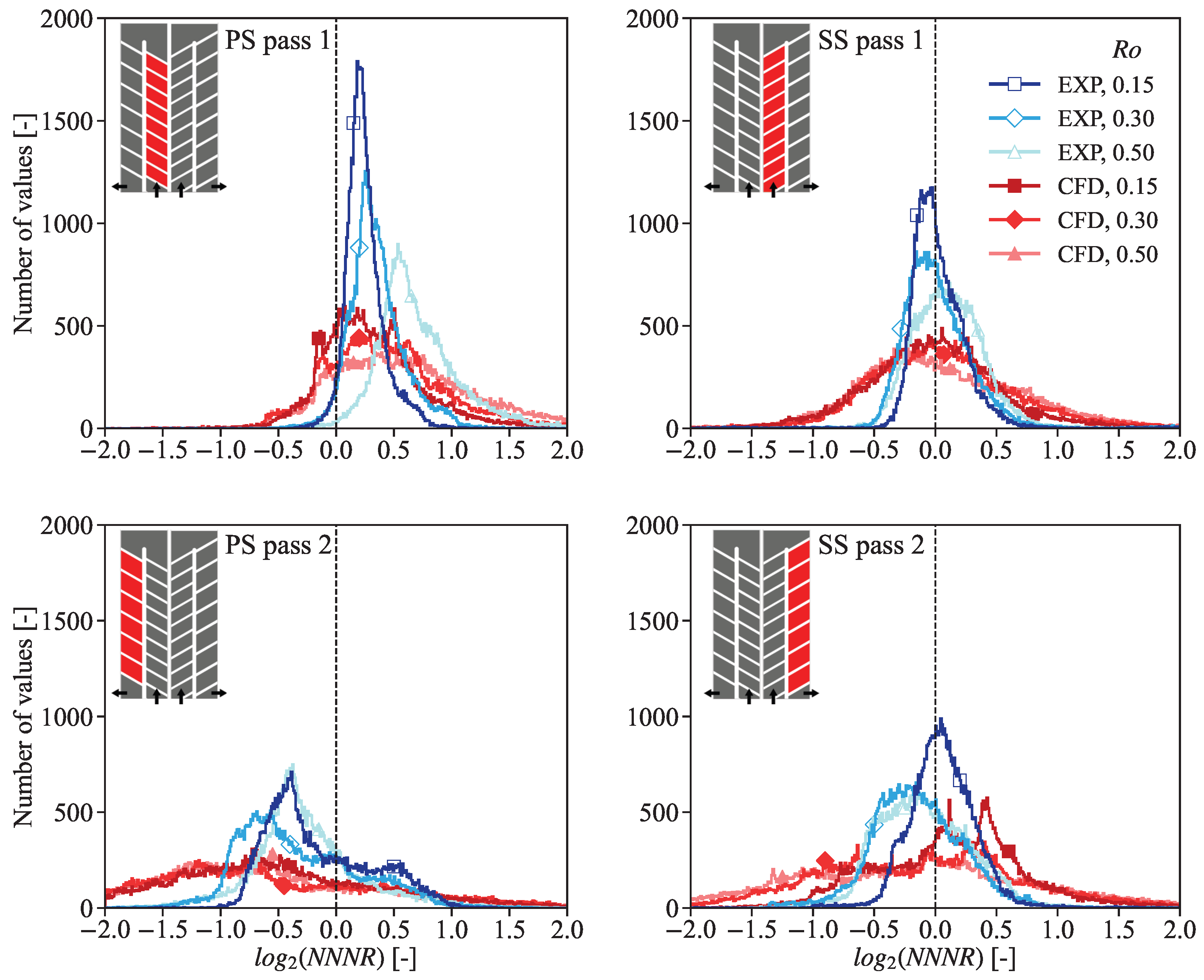
9.3. Rotational Effect

In Section 9.1, the rotationally induced heat transfer footprint was examined for the test case of $Ro\approx 0.15$ and $\alpha =+8^{°}$. As shown in Figure 8, the local rotational features vary significantly depending on the considered region of the cooling channel. Later, in Section 9.2, variation in the angle of attack exposed a remarkable influence on the local heat transfer structure for the PS, as well as for the SS, especially in pass 1. Contrarily, an increase in the rotational speed is not expected to modify the structure dramatically but boost or diminish the overall heat transfer rates while preserving its original shape. Considering the nominal angle of attack, a variation in the rotation number from $Ro\approx 0.15$ up to $Ro\approx 0.50$ is examined in the following.

In Figure 12, heat transfer data are presented via contour plots of $lo{g}_2$(NNNR) for increasing rotational speeds from left to right. As noted in Section 9.1 for $Ro\approx 0.15$, heat transfer augmentation dominates in PS pass 1. By further increasing the rotational speed, this effect is intensified so that the highest heat transfer rates are achieved for $Ro\approx 0.50$, with a remarkable enhancement in the first rib segments. At the top left-hand side of Figure 13, the $lo{g}_2$(NNNR) histogram for PS pass 1 confirms the latter remark. Clearly, the increase in rotational speed shifts the peak of the value count towards higher heat transfer values. Moreover, as $Ro$ is increased the distributions tend to flatten out and become broader, covering a wider range of $lo{g}_2$(NNNR) values. As noted by the contour plots presented in Figure 12, local spots where heat transfer decrease comes into view (B1) remain throughout all the investigated rotation numbers. These spots can also be observed in the CFD contour plots at the bottom. It is worth mentioning that their location and size are correctly predicted in the first rib segments, yet further downstream, the agreement between the TLC experiment and numerical simulation is reduced. Here, the CFD model locally overestimates the rotational effect on heat transfer rates, displaying relatively broad regions where rotationally induced heat transfer decrease dominates, i.e., $lo{g}_2\left(\mathit{NNNR}\right)<0\to \mathit{NNNR}<1$. In PS pass 2, areas with rotationally driven heat transfer augmentation appear to shrink with increasing rotational speed, in favor of regions with heat transfer decrease, as evidenced by B3 and B2 in Figure 12.

Disregarding local effects, the key trends observed for PS at different rotation numbers can be summarized by means of the segment-averaged representation presented in Figure 14a. As a general remark, an increase in $Ro$ leads to an augmentation in the rotationally driven heat transfer rates ($lo{g}_2\left(\mathit{NNNR}\right)$) for pass 1. The opposite holds true for pass 2. The increase in heat transfer rates in pass 1 is especially pronounced from $Ro\approx 0.30$ to $Ro\approx 0.50$. Clearly, the rotationally induced heat transfer enhancement consistently decreases along the channel length, displaying the highest $lo{g}_2$(NNNR) values at the channel inlet and the lowest values at the outlet, as experimental and numerical data reflect. There exists a turning point in the bend region, whereupon heat transfer rates turn from positive ($lo{g}_2\left(\mathit{NNNR}\right)>0$) to negative ($lo{g}_2\left(\mathit{NNNR}\right)<0$) and further decrease until the channel outlet is reached. The numerical model yields qualitatively reliable predictions of these trends; however, the heat transfer augmentation in the first section of pass 1 and in the last section of pass 2 is generally underpredicted, especially for $Ro\approx 0.50$. According to the experimental results, the maximum enhancement occurs in the first rib segment in streamwise direction ($-8$, pass 1), from $lo{g}_2\left(\mathit{NNNR}\right)\approx 0.41\to \mathit{NNNR}\approx 1.33$ ($Ro\approx 0.15$) up to $lo{g}_2\left(\mathit{NNNR}\right)\approx 1.2\to \mathit{NNNR}\approx 2.30$ ($Ro\approx 0.50$). Contrarily, the strongest heat transfer decrease arises for rib segment 5 in pass 2, from $lo{g}_2\left(\mathit{NNNR}\right)\approx -0.28\to \mathit{NNNR}\approx 0.82$ ($Ro\approx 0.15$) down to $lo{g}_2\left(\mathit{NNNR}\right)\approx -0.59\to \mathit{NNNR}\approx 0.66$ ($Ro\approx 0.30$).

With regard to the SS of the cooling channel, subtle changes transpire in the heat transfer structure due to rotation (see Figure 12). As for SS pass 1, the surfaces adjacent to the leading edge (B4) experience a heat transfer increase as a result of rotation for all considered rotation numbers, while the remaining areas (B5) experience a decrease in $lo{g}_2$(NNNR) for $Ro\approx 0.15$ and $Ro\approx 0.30$. Additionally, for the highest rotation number ($Ro\approx 0.50$), a new region appears adjacent to the inner wall separator (B6) where the increase in rotationally induced heat transfer dominates. By considering the histogram at the top right-hand side of Figure 13, we appreciate a slight yet systematic broadening of the distributions in both directions and a tendency to shift the distributions’ peaks towards higher heat transfer rates through increases in $Ro$ for the experimental and, to a lesser extent, numerical results.

Whereas the increase in rotational speed proved to be slightly beneficial for SS pass 1 in terms of increased heat transfer rates, it appears to be detrimental for SS pass 2. Generally, the surfaces where heat transfer enhancement dominates tend to shrink in favor of heat transfer reduction, as observed in region B7 in Figure 12. Furthermore, sharper $lo{g}_2$(NNNR) gradients appear with an increase in $Ro$. These remarks are supported by the histogram plot at the bottom right-hand side of Figure 13. The increase in rotation number leads to a peak shift to the left, i.e., towards lower $lo{g}_2$(NNNR) values, and the distribution widens in this direction, as evidenced by both experimental and numerical results. Segment-averaged data for the suction side (see Figure 14b) reveal an increase in $lo{g}_2$(NNNR) for the first segments of pass 1 and a strong decrease for the most downstream segments in pass 2 with increasing rotation number. Generally, segment-averaged data for SS is limited to a band of $\mathit{NNNR}=1.0\pm 0.5$, which contrasts with the broader spectrum of heat transfer rates for PS.

10. Conclusions

This study set out to gain a better understanding of the internal convective heat transfer characteristics in a generic two-pass cooling channel under engine-similar rotating conditions. In addition to the experimental approach based on transient TLC measurements, we introduce a numerical method based on steady-state RANS simulations, which effectively supports the experiment.

Preliminary heat transfer results for the nominal angle of attack ($\alpha =+8^{°}$) with rotation ($Ro\approx 0.15$) disclosed a remarkable local heat transfer enhancement as high as $Nu/N{u}_0\approx 7$ relative to the smooth channel flow. Furthermore, the heterogeneous impact of rotation on the different channel regions was revealed. Considering the exemplary radially outward flow in the first passage, the PS experiences an overall rotationally induced increase in heat transfer. Contrarily, the SS is split in two regions, i.e., the surfaces adjacent to the leading edge, where heat transfer enhancement dominates, and the surfaces next to the inner wall separator, where heat transfer is decreased.

The presented numerical approach was validated against locally resolved experimental heat transfer data under rotation. Variation in the angle of attack triggers a new Coriolis force direction, which results in major changes in the heat transfer structure, with the most significant differences occurring with an angle of attack of $+{46.5}^{°}$ relative to the other angles. For all considered channel orientations, the numerical model was able to reproduce the correct sign of $lo{g}_2\left(\mathit{NNNR}\right)$ from the experimental results with minor deviations and with an overall satisfactory agreement. The most noticeable inconsistencies between experimental and numerical results arose at the bend region, where the flow field exhibits a complex structure due to the transition from a trapezoidal to rectangular cross-section. One of the most significant findings to emerge from this experimental–numerical study is the sharper gradient observed in the CFD $lo{g}_2\left(\mathit{NNNR}\right)$ contours, which could later be confirmed in the broader histogram distributions. A potential explanation for this phenomenon is the three-dimensional nature of heat conduction, which might be dominant in the TLC experiment but is not corrected (one-dimensional assumption).

A sensitivity study on the rotational speed proved that a higher $Ro$ mainly has an enhancing or diminishing effect on heat transfer rates, while the local heat transfer structure is preserved. In particular, PS pass 1 showed a clear tendency of heat transfer enhancement, with averaged rotationally induced heat transfer rates as high as $lo{g}_2\left(\mathit{NNNR}\right)\approx 1.2\to +130\%$ for $Ro\approx 0.50$. In other channel regions, such as PS pass 2 and SS pass 2, the effect was primarily detrimental. Histogram plots confirmed the qualitative observations derived from the contour plots, and area-averaged representation allowed for quantification of the results.

In view of the findings reported here, the proposed numerical method qualifies for accurate heat transfer predictions under different operating conditions, and its usage is recommended by the authors for upcoming investigations. The results of this research underscore the importance of rotation as a central aspect shaping the local heat transfer structure within internal cooling channels. If considered in the development process through, e.g., optimized turbulator designs, the rotational effect could potentially enable reduced coolant consumption in the future, with a subsequent increase in the thermal efficiency.

References

- Han, J.C. Fundamental Gas Turbine Heat Transfer. J. Therm. Sci. Eng. Appl. 2013, 5, 021007. [Google Scholar] [CrossRef]
- Ligrani, P. Heat Transfer Augmentation Technologies for Internal Cooling of Turbine Components of Gas Turbine Engines. Int. J. Rotating Mach. 2013, 2013, 275653. [Google Scholar] [CrossRef]
- Wagner, J.H.; Johnson, B.V.; Hajek, T.J. Heat Transfer in Rotating Passages with Smooth Walls and Radial Outward Flow. J. Turbomach. 1991, 113, 42–51. [Google Scholar] [CrossRef]
- Johnson, B.; Wagner, J.; Steuber, G.; Yeh, F. Heat transfer in rotating serpentine passages with selected model orientation for smooth or skewed trip walls. Int. J. Turbomach. 1994, 116, 738–744. [Google Scholar] [CrossRef]
- Zhou, F.; Lagrone, J.; Acharya, S. Internal Cooling in 4:1 AR Passages at High Rotation Numbers. In Turbo Expo: Power for Land, Sea, and Air; American Society of Mechanical Engineers: New York, NY, USA, 2004; pp. 451–460. [Google Scholar] [CrossRef]
- Chang, S.W.; Yang, T.L.; Wang, W.J. Heat Transfer in a Rotating Twin-Pass Trapezoidal-Sectioned Passage Roughened by Skewed Ribs on Two Opposite Walls. Heat Transf. Eng. 2006, 27, 63–79. [Google Scholar] [CrossRef]
- Huh, M.; Lei, J.; Liu, Y.H.; Han, J.C. High Rotation Number Effects on Heat Transfer in a Rectangular (AR = 2:1) Two-Pass Channel. J. Turbomach. 2010, 133, 021001. [Google Scholar] [CrossRef]
- Wright, L.M.; Yang, S.F.; Wu, H.W.; Han, J.C.; Lee, C.P.; Azad, S.; Um, J. Heat Transfer in a Rotating, Blade-Shaped Serpentine Cooling Passage With Discrete Ribbed Walls at High Reynolds Numbers. J. Heat Transf. 2019, 142, 012002. [Google Scholar] [CrossRef]
- Ekkad, S.V.; Singh, P. Detailed Heat Transfer Measurements for Rotating Turbulent Flows in Gas Turbine Systems. Energies 2021, 14, 39. [Google Scholar] [CrossRef]
- Ekkad, S.V.; Singh, P. Liquid Crystal Thermography in Gas Turbine Heat Transfer: A Review on Measurement Techniques and Recent Investigations. Crystals 2021, 11, 1332. [Google Scholar] [CrossRef]
- Lorenzon, A.; Casarsa, L. Validation of the Transient Liquid Crystal Thermography Technique for Heat Transfer Measurements on a Rotating Cooling Passage. Energies 2020, 13, 4759. [Google Scholar] [CrossRef]
- Waidmann, C.; Poser, R.; Nieland, S.; von Wolfersdorf, J. Design of a Rotating Test Rig for Transient Thermochromic Liquid Crystal Heat Transfer Experiments. In Proceedings of the ISROMAC 2016, International Symposium on Transport Phenomena and Dynamics of Rotating Machinery, Honolulu, HI, USA, 10–15 April 2016; Available online: https://hal.science/hal-01884257v1 (accessed on 20 November 2023).
- Waidmann, C.; Poser, R.; Göhring, M.; von Wolfersdorf, J. First Operation of a Rotating Test Rig for Transient Thermochromic Liquid Crystal Heat Transfer Experiments. In Proceedings of the XXIV Biannual Symposium on Measuring Techniques in Turbomachinery Transonic and Supersonic Flow in Cascades and Turbomachines, Prague, Czech Republic, 30–31 August 2018; Available online: https://www.meastechturbo.com/paper-archives/item/344-first-operation-of-a-rotating-test-rig-for-transient-thermochromic-liquid-crystal-heat-transfer-experiments (accessed on 20 November 2023).
- Waidmann, C. Heat Transfer Measurements in Rotating Turbine Blade Cooling Channel Configurations Using the Transient Thermochromic Liquid Crystal Technique. Ph.D. Thesis, University of Stuttgart, Stuttgart, Germany, 2020. Available online: https://elib.uni-stuttgart.de/handle/11682/11344 (accessed on 20 November 2023).
- Waidmann, C.; Poser, R.; Gutiérrez de Arcos, D.; Göhring, M.; von Wolfersdorf, J.; Semmler, K.; Jäppelt, B. Experimental Investigation of Local Heat Transfer in a Rotating Two-Pass Cooling Channel Using the Transient Thermochromic Liquid Crystal (TLC) Technique. In Proceedings of the ASME Turbo Expo 2022: Turbomachinery Technical Conference and Exposition, Rotterdam, The Netherlands, 13–17 June 2022; Volume 6B: Heat Transfer—General Interest/Additive Manufacturing Impacts on Heat Transfer; Internal Air Systems; Internal Cooling, p. V06BT15A009. Available online: https://asmedigitalcollection.asme.org/GT/proceedings-abstract/GT2022/86045/V06BT15A009/1149022 (accessed on 20 November 2023).
- Gutiérrez de Arcos, D.; Waidmann, C.; Poser, R.; von Wolfersdorf, J.; Jäppelt, B. Comparison of Experimental and Numerical Local Rotational Heat Transfer Effects in a Two-Pass Cooling Channel Configuration. In Proceedings of the ASME Turbo Expo 2022: Turbomachinery Technical Conference and Exposition, Rotterdam, The Netherlands, 13–17 June 2022; Volume 6B: Heat Transfer—General Interest/Additive Manufacturing Impacts on Heat Transfer; Internal Air Systems; Internal Cooling. p. V06BT15A008. Available online: https://asmedigitalcollection.asme.org/GT/proceedings-abstract/GT2022/86045/V06BT15A008/1148975 (accessed on 20 November 2023).
- Gutiérrez de Arcos, D.; Waidmann, C.; Poser, R.; von Wolfersdorf, J.; Jäppelt, B.; Semmler, K. Effect of protrusions and leading edge ribs on the local heat transfer characteristics in a two-pass cooling channel under rotation. In Proceedings of the GPPS Technical Conference, Chania, Greece, 4–6 September 2024; Available online: https://www.researchgate.net/publication/384361224_Effect_of_protrusions_and_leading_edge_ribs_on_the_local_heat_transfer_characteristics_in_a_two-pass_cooling_channel_under_rotation (accessed on 10 December 2023).
- Pagnacco, F.; Furlani, L.; Armellini, A.; Casarsa, L.; Davis, A. Rotating Heat Transfer Measurements on Realistic Multi-pass Geometry. Energy Procedia 2016, 101, 758–765. [Google Scholar] [CrossRef]
- Pearce, R.; Ireland, P.; He, L.; McGilvray, M.; Romero, E. Computational and Experimental Study of Heat Transfer in Rotating Ribbed Radial Turbine Cooling Passages. In Turbo Expo: Power for Land, Sea, and Air; American Society of Mechanical Engineers: New York, NY, USA, 2015; Volume 5A: Heat Transfer, p. V05AT11A026. Available online: https://asmedigitalcollection.asme.org/GT/proceedings-abstract/GT2015/56710/V05AT11A026/237166 (accessed on 20 November 2023).
- Massini, D.; Burberi, E.; Carcasci, C.; Cocchi, L.; Facchini, B.; Armellini, A.; Casarsa, L.; Furlani, L. Effect of rotation on a gas turbine blade internal cooling system: Experimental investigation. J. Eng. Gas Turbines Power 2017, 139, 101902. [Google Scholar] [CrossRef]
- Burberi, E.; Massini, D.; Cocchi, L.; Mazzei, L.; Andreini, A.; Facchini, B. Effect of rotation on a gas turbine blade internal cooling system: Numerical investigation. J. Turbomach. 2017, 139, 031005. [Google Scholar] [CrossRef]
- Duchaine, F.; Gicquel, L.; Grosnickel, T.; Koupper, C. Large-Eddy simulation of the flow developing in static and rotating ribbed channels. J. Turbomach. 2020, 142, 041003. [Google Scholar] [CrossRef]
- Singh, P.; Sarja, A.; Ekkad, S.V. Experimental and Numerical Study of Chord-Wise Eight-Passage Serpentine Cooling Design for Eliminating the Coriolis Force Adverse Effect on Heat Transfer. J. Therm. Sci. Eng. Appl. 2021, 13, 011026. [Google Scholar] [CrossRef]
- Murata, A.; Mochizuki, S. Effect of centrifugal buoyancy on turbulent heat transfer in an orthogonally rotating square duct with transverse or angled rib turbulators. Int. J. Heat Mass Transf. 2001, 44, 2739–2750. [Google Scholar] [CrossRef]
- Abdel-Wahab, S.; Tafti, D.K. Large eddy simulation of flow and heat transfer in a 90 deg ribbed duct with rotation: Effect of Coriolis and centrifugal buoyancy forces. J. Turbomach. 2004, 126, 627–636. [Google Scholar] [CrossRef]
- Sewall, E.A.; Tafti, D.K. Large Eddy Simulation of Flow and Heat Transfer in the Developing Flow Region of a Rotating Gas Turbine Blade Internal Cooling Duct With Coriolis and Buoyancy Forces. J. Turbomach. 2007, 130, 011005. [Google Scholar] [CrossRef]
- Saravani, M.S.; DiPasquale, N.J.; Beyhaghi, S.; Amano, R.S. Heat transfer in internal cooling channels of gas turbine blades: Buoyancy and density ratio effects. J. Energy Resour. Technol. 2019, 141, 112001. [Google Scholar] [CrossRef]
- Göhring, M.; Krille, T.; Feile, J.; von Wolfersdorf, J. Heat Transfer Predictions in Smooth and Ribbed Two-Pass Cooling Channels under Stationary and Rotating Conditions. In Proceedings of the 16th International Symposium on Transport Phenomena and Dynamics of Rotating Machinery, Honolulu, HI, USA, 10–15 April 2016; Available online: https://hal.science/hal-01884254 (accessed on 20 November 2023).
- Göhring, M.; Hartmann, C.; von Wolfersdorf, J. Numerical Investigation of Transient Heat Transfer Experiments Under Rotation. Turbo Expo: Power for Land, Sea, and Air; American Society of Mechanical Engineers: New York, NY, USA, 2018; Volume 5A: Heat Transfer, p. V05AT11A011. Available online: https://asmedigitalcollection.asme.org/GT/proceedings-abstract/GT2018/51081/V05AT11A011/272426 (accessed on 20 November 2023).
- Göhring, M. Numerical Investigation of Internal Two-Pass Gas Turbine Cooling Channels Under the Influence of Rotation. Ph.D. Thesis, University of Stuttgart, Stuttgart, Germany, 2020. Available online: https://elib.uni-stuttgart.de/handle/11682/11076 (accessed on 20 November 2023).
- Steurer, A.; Poser, R.; von Wolfersdorf, J.; Retzko, S. Application of the Transient Heat Transfer Measurement Technique Using Thermochromic Liquid Crystals in a Network Configuration with Intersecting Circular Passages. J. Turbomach. 2019, 141, 051010. [Google Scholar] [CrossRef]
- Jenkins, S.C.; Shevchuk, I.V.; von Wolfersdorf, J.; Weigand, B. Transient Thermal Field Measurements in a High Aspect Ratio Channel Related to Transient Thermochromic Liquid Crystal Experiments. J. Turbomach. 2012, 134, 031002. [Google Scholar] [CrossRef]
- Waidmann, C.; Poser, R.; von Wolfersdorf, J.; Fois, M.; Semmler, K. Investigations of heat transfer and pressure loss in an engine-similar two-pass internal blade cooling configuration. In Proceedings of the 10th European Conference on Turbomachinery Fluid dynamics & Thermodynamics, European Turnomachinery Society, Lappeenranta, Finland, 15–19 April 2013; Available online: https://www.euroturbo.eu/publications/proceedings-papers/etc2013-168 (accessed on 20 November 2023).
- Ireland, P.T.; Jones, T.V. Liquid crystal measurements of heat transfer and surface shear stress. Meas. Sci. Technol. 2000, 11, 969–986. [Google Scholar] [CrossRef]
- Poser, R.; von Wolfersdorf, J.; Semmler, K. Transient Heat Transfer Experiments in Complex Passages. In Proceedings of the HT2005 ASME Summer Heat Transfer Conference, San Francisco, CA, USA, 17–22 July 2005; Available online: https://asmedigitalcollection.asme.org/HT/proceedings-abstract/HT2005/47314/797/313393 (accessed on 20 November 2023).
- Poser, R.; von Wolfersdorf, J.; Lutum, E. Advanced evaluation of transient heat transfer experiments using thermochromic liquid crystals. Proc. Inst. Mech. Eng. Part J. Power Energy 2007, 221, 793–801. Available online: https://journals.sagepub.com/doi/10.1243/09576509JPE464 (accessed on 20 November 2023). [CrossRef]
- Poser, R.; Ferguson, J.R.; von Wolfersdorf, J. Temporal Signal Preprocessing and Evaluation of Thermochromic Liquid Crystal Indications in Transient Heat Transfer Experiments. In Proceedings of the 8th European Conference on Turbomachinery Fluid Dynamics and Thermodynamics, Graz, Austria, 23–27 March 2009; pp. 785–795. [Google Scholar]
- Poser, R.; von Wolfersdorf, J. Transient Liquid Crystal Thermography in Complex Internal Cooling Systems; VKI Lecture Series—Internal Cooling in Turbomachinery; von Karman Institute for Fluid Dynamics: Brussels, Belgium, 2010. [Google Scholar]
- Taler, J.; Duda, P. Solving Direct and Inverse Heat Conduction Problems; Springer: Berlin/Heidelberg, Germany, 2006. [Google Scholar]
- Myers, G. Analytical Methods in Conduction Heat Transfer, 2nd ed.; Genium Publishing Corp.: New York, NY, USA, 1998. [Google Scholar]
- White, F.M.; Majdalani, J. Preliminary Concepts. In Viscous Fluid Flow; McGraw-Hill: New York, NY, USA, 2006; Volume 3, Chapter 1. [Google Scholar]
- ANSYS Inc. ANSYS CFX Theory Guide; ANSYS Inc.: Canonsburg, PA, USA, 2021; Release 21.2. [Google Scholar]
- ANSYS Inc. ANSYS ICEM CFD User’s Manual; ANSYS Inc.: Canonsburg, PA, USA, 2016; Release 17.1. [Google Scholar]
- Incropera, F.P.; DeWitt, D.P.; Bergman, T.L.; Lavine, A.S. Fundamentals of Heat and Mass Transfer, 7th ed.; International Student version ed.; Wiley: Singapore, 2013. [Google Scholar]
- Williams, W.C. If the Dittus and Boelter equation is really the McAdams equation, then should not the McAdams equation really be the Koo equation? Int. J. Heat Mass Transf. 2011, 54, 1682–1683. [Google Scholar] [CrossRef]
- Liou, T.M.; Chen, C.C.; Chen, M.Y. Rotating effect on fluid flow in two smooth ducts connected by a 180-degree bend. J. Fluids Eng. 2003, 125, 138–148. [Google Scholar] [CrossRef]
- Crowder, S.; Delker, C.; Forrest, E.; Martin, N. Introduction to Statistics in Metrology; Springer: Berlin/Heidelberg, Germany, 2020. [Google Scholar]
- Forster, M.; Seibold, F.; Krille, T.; Waidmann, C.; Weigand, B.; Poser, R. A Monte Carlo approach to evaluate the local measurement uncertainty in transient heat transfer experiments using liquid crystal thermography. Measurement 2022, 190, 110648. [Google Scholar] [CrossRef]
- Brandrup, J.; Immergut, E.H.; Grulke, E.A.; Abe, A.; Bloch, D.R. Polymer Handbook; Wiley: New York, NY, USA, 1999; Volume 89. [Google Scholar]