1. Introduction
In today’s competitive world, higher education (HE) institutions need to deliver efficient and quality education to retain their students. The extensive blending of digital technologies into HE teaching and learning environments has resulted in large amounts of student data that can provide a longer-term picture of student learning behaviours. To understand and assist student learning, HE providers are implementing learning analytics (LA) systems; these systems provide data-driven insights about students to assist educators in determining their overall academic progression. This technology is particularly being leveraged to predict at-risk students and identify their learning problems at early stages, with the purpose of initiating timely interventions and tailoring education [
1,
2,
3] to each student’s level of need.
LA approaches typically rely on educational data collected from various learning activities provided via online learning platforms, such as learning management systems (LMSs) [
4]. LMSs are web-based learning systems that offer a virtual platform for facilitating teaching and learning, such as providing students with online course content, tracking student interactions, enabling peer communication over online forums, delivering course assessments to students, or releasing assessment grades [
5]. Various stakeholders have different objectives for using an LMS. For instance, Romero and Ventura [
6] suggest that students use an LMS to personalise their learning, such as review specific material or engage in relevant discussions as they prepare for their exams. Meanwhile, teachers rely on an LMS to deliver their course content and manage teaching resources in a relatively simple and uniform manner [
7] without worrying about pace, place or space constraints. Irrespective of how an LMS is used, user interaction with the system generates significant and detailed digital footprints that can be mined using LA tools.
The most widely used open source LMS is Moodle (i.e., Modular Object-Oriented Dynamic Learning Environment). It facilitates instructors to create online lessons that can be used in any of the three delivery modes: face-to-face, entirely online, or blended [
5]. Moodle is mostly used as a communication platform for educators to communicate with students, as well as to publish course materials and grade student assignments. Students can therefore benefit from Moodle by having more interactions with their instructor and their peers, as they engage with the course content. Every activity performed in Moodle is captured in a database or system log, which can then be analysed to examine underlying student learning behaviours via LA approaches. A deeper investigation may be conducted if any indicators pertaining to at-risk students are identified [
7]. A modelling process translates these indicators (extracted from training data) into predictive insights, which can be used on new data (or test data) to gauge student online behaviours. Teachers can then support at-risk students in overcoming their learning difficulties [
8].
Most of the research into predicting student performance and identifying at-risk students has focused on developing tailor-made models for different courses. There are multiple problems with this approach, such as the issue of scalability and overhead in developing, optimising and maintaining custom models for each course within the HE provider’s vast array of course offerings. This approach brings to the fore both human resource and technical expenses. Even if these challenges can be overcome, course-specific models are likely to perform poorly across numerous courses due to data insufficiency, resulting in overfitting. This is a tendency for courses that may have small cohorts, or for courses that have been newly set up and thus do not have historic data from which patterns can be learned through machine learning.
An alternative approach is to develop generic predictive models that operate across all of the disparate courses, though only a few works have attempted this strategy to date [
9]. This is a technically more challenging approach due to the fact that more experimental rigour is required in the feature engineering phase, whereby more generic and abstract features that describe students’ learning patterns need to be devised in a way that they are course-agnostic. The present study focuses on building a generic (or portable) model using a machine learning algorithm to generate a classifier for predicting student final outcomes.
Therefore, the motivation of this study is to demonstrate how a generic, course-agnostic predictive model can be developed that has strong portability attributes and can thus be effective at predicting students’ final outcomes across disparate courses. Furthermore, this research demonstrates how an effective model can be built using a variety of student attributes that range from demographic to those that capture students’ academic performances. We perform numerous experiments by developing models at different time frames (two, four, six and eight weeks into a course) to examine how early in the course an effective prediction can be made. Our experiments involve multiple algorithms, and we note the CatBoost algorithm as being the most effective on our dataset.
Against this backdrop, the rest of the paper is organised as follows. The next section reviews existing studies on LA, with emphasis on the various machine learning techniques used to predict students’ academic performance. Next, the datasets used in this study are described, followed by our proposed algorithmic approach. The results are then presented, findings are discussed, and conclusions are made thereafter.
2. Review of Related Studies
Prediction of student academic performance has drawn considerable attention in the educational field. For instance, predicting whether a student will pass or fail a course, and then notifying the instructor about the at-risk student, can enable the instructor to intervene and provide the student with learning pathways to improve their performance [
10]. Several studies have reported success in predicting student academic performance using various educational data mining techniques. This review covers related works on prediction using a generic (or course-agnostic) model and early prediction techniques within the scope of the study.
2.1. Related Study Exploring Prediction Using Generalised Model
Chen and Cui [
11] applied a deep learning approach—long short-term memory (LSTM) networks—to analyse student online behaviours for early prediction of course performance using the students’ LMS data. The prediction performance of the LSTM networks approach was compared against eight conventional machine learning classifiers and AUC was used as the evaluation metric. The model generalisability was evaluated using the data derived from semester 1 and semester 2. The results showed that test AUC scores for semester 1 were around 0.75, which was higher than those obtained for semester 2, as the training data was also from the course in semester 1.
The motivation of Zambrano et al. [
9] was to study the portability of student performance where the knowledge extracted from a specific course can be applied directly to a different course from the same degree and with similar levels of LMS usage. Using J48 decision trees, the authors created a predictive model based on 24 courses to classify the students into a pass or fail category. The model achieved an AUC loss value of 0.09 and 0.28 when using the courses to the same degree, and an AUC loss range from 0.22 to 0.25 for courses with similar levels of Moodle usage.
LMS data and in-between assessment grades were used in another study [
7] to predict student performance. Multiple linear regression was used to induce predictive models at the end of the course and evaluate the efficacy of the available features within LMS. To assess whether the data could offer an intervention during a course, linear and logistic regression was applied to the features at the end of each week of the course. The results showed the LMS usage data to be a weak predictor here unless other assessment data were also included, which ultimately improved predictions.
In another study by Nakayama et al. [
12], the performance of students in a blended learning course was predicted based on their note-taking activities and their individual characteristics, which were measured via student surveys. The possibility of predicting performance in final exams was evaluated by using the features of the contents of notes taken by students throughout the course and overall participant characteristics. The results showed that features of note-taking activities play a major role in predicting the final exam scores.
Gasevic et al. [
13] built different logistic regression models for nine undergraduate courses to predict student performance (pass or fail). They used LMS logs and student information from the institutional student information system to build one model that would cover all the courses, as well as one model per course. The authors computed the area under the ROC (receiving operating characteristic) curve (AUC) values. The generalised model for all the courses showed an acceptable accuracy (0.5 ≤ AUC < 0.7). However, the models specifically built for a particular course achieved excellent (0.8 ≤ AUC < 0.9) or outstanding (AUC ≥ 0.9) performances.
2.2. Related Study Exploring Early Prediction of Student Performance
The main reason to predict student performance is to identify the at-risk students, intervening and customising learning strategies in time to support them in achieving better results; however, most earlier studies have focused on predicting students’ final course results once all the student course data was gathered, which would leave no time for such interventions. Upon recognising this issue, more researchers have recently attempted to predict student outcomes earlier in their course of study. For instance, González et al. [
14] tried to identify struggling learners at early stages of the course. They used LMS data to predict student performance at set points along the way, when 10%, 25%, 33% and 50% of the course had been completed. Different classification algorithms, namely Decision Tree (DT), Naïve Bayes (NB), Logistic Regression (LR), Multilayer Perceptron (MLP), and Support Vector Machine (SVM), were used to evaluate the prediction accuracy. MLP achieved the best performance on this dataset, with 80% accuracy when 10% of the course had been delivered and 90% accuracy when half of the course had been completed.
A solution proposed by Queiroga et al. [
14] used students’ interaction with their virtual learning environment to identify at-risk students as early as possible. Classic DT, MLP, LR, random forest (RF), and the meta-algorithm AdaBoost (ADA) were used. The proposed approach utilised genetic algorithms (GA) to tune the hyperparameters of the classifiers, and the results were compared with the traditional method without hyperparameter optimisation. The prediction model was run every two weeks for a 50-week duration course. The results showed that the highest AUC score was achieved using the GA during the initial period. There was a considerable decrease in performance from week 30 due to the increase in the number of input attributes.
A study by Zhao et al. [
15] used Moodle data to predict student performance in the first quarter of a semester. They used the fuzzy rule-based classification method (FRBCS) and a modified FRBCS to predict the learning outcomes of students. The results showed that the modified FRBCS method provided higher stability and better performance compared to the unmodified FRBCS method.
A study made by Ramaswami et al. [
16] tried to estimate the earliest possible time within a course at which reliable identification of students at risk could be made. The input data were a combination of LMS, demographics and assignment grades. Four different classifier algorithms were tested: NB, RF, LR and k-Nearest Neighbours (kNN). Two experiments were conducted, one using all the features and the other using features selected for their high prediction accuracy. LR produced the best accuracy of 83% in week 11, and the authors noted that it is better to apply feature selection approaches rather than select all features for making predictions due to overfitting.
Howard et al. [
17] attempted to determine the ideal time to apply an early warning system in a course. LMS data along with student grades and their demographic information were used as input data for the prediction model. After testing multiple predictive models, the Bayesian additive regressive trees (BART) model yielded the best results with a mean absolute error (MAE) of 6.5% as early as week 6, precisely midway through the course. This point in the course is sufficiently early so that remedial measures can be taken by the teacher, as required.
To sum up, various models have been proposed by researchers and a variety of different machine learning approaches have been used to mine educational data for student performance prediction. Moreover, some excellent results have been achieved using an assortment of different methods, with no one method outshining all other methods (refer to
Table 1), unsurprisingly in line with the “No Free Lunch” theorem [
18]. In general, a recent systematic literature review [
10] into predicting student performance has found that reported accuracies range widely and are influenced by many factors, with the bulk of the studies appearing to achieve predictive accuracies between ~70% to ~90%.
3. Datasets
The data used in this exploratory research was extracted from courses offered at an Australasian HE institution in a blended learning environment. Tayebinik and Puteh [
20] have defined blended learning as a fusion of traditional face-to-face and online learning, where instructional delivery happens across both traditional and online courses, such that the online component becomes a natural extension of traditional learning. Data from various semesters were included in building the prediction model. The purpose of considering courses of different durations was to make sure our models could handle courses of different lengths and attributes. Single course-specific predictive models are commonly able to provide better performance when they have sufficient historic data, but they are not easily scalable to port to other courses. Data from the LMS (Moodle) action logs, the Student Management System (SMS) and the Enrolment Management System (EMS) were used for the study. These are described next.
3.1. Action Logs from Moodle
Moodle’s built-in features track student activities in each course [
21]. The courses comprise online modules pertaining to subject readings (provided via book resources, URL links or web pages), assessments (in the form of assignments or quizzes) and forum discussions. For the purposes of this study, the log data directly related to student activities were extracted from Moodle, while instructor data were excluded.
Each event record in the log signifies various actions (started, viewed, created, updated, etc.) performed by students on Moodle; data related to eight types of learning activities were collected.
Table 2 shows the percentage of various activities logged by course. It should be noted that the usage of these activities varies across courses, and not all activities may be relevant for every course.
For instance, quiz activities do not form part of many courses, such as for Internet Programming or Application Software Development courses, amongst a few others; therefore, log data are not available for them (see
Table 2). Numerical representations were calculated for each course module.
3.2. Enrolment Management System
The usage of the LMS and therefore the amount of logged data is scarcer in earlier parts of a course, which can be expected to lead to a lower predictive accuracy at initial stages of a course. Hence, demographic information and pre-academic data, such as age, gender, citizenship and entrance requirements, from the EMS were also utilised to augment the total dataset.
3.3. Student Management System
The SMS provided assessment data consisting of in-between assignment grades, quizzes, final exams and total course marks. Some of the assessments were online and logged in the Moodle LMS, while other assessments were offline and handed in on paper or via other systems.
4. Method
Before the students’ data could be accessed for conducting any form of analysis, ethics approval was required. An ethics application was submitted to the Human Research Ethics Committee at the host HE institution, and subsequently, approval to proceed was attained.
Once the data were obtained, a design decision was made to use a derivative of the final course mark for each student as the target (or dependent) variable for prediction. The final course mark is based on weighted averages of the marks that students received from the online assignments and the final examination.
Student support services at the given institution require predictive outputs that indicate only two possible outcomes for each student, namely if they are at risk or otherwise. Therefore, in order to conduct machine learning, each student in the historic dataset record needed to be labelled as being either at risk or not. A subsequent design decision needed to be made on how to define each of these two categories so that models could be generated. An early assumption was made that students with a mean final course mark of 50% or less were likely to be at-risk students due to the fact that these students have not successfully completed numerous courses. However, initial experiments using this threshold yielded highly imbalanced datasets and consequently poor models.
Subsequently, the threshold for defining at-risk students was adjusted and fixed at 60% or less for a mean final course mark, with the remainder being considered not at-risk. This threshold decision was supported by the underlying data, which revealed that the mean course mark for students who eventually abandoned their qualification studies was 61%, and only 15% of students who eventually completed their qualification studies achieved a mean course mark of 60% or less. The adjusted threshold addressed the class imbalance problem to a sufficient degree since most machine learning algorithms can handle some imbalance, and standard performance evaluation measures can still be effective unless large amounts of imbalance exist [
22].
The raw data from the LMS log files were processed in order to engineer features used for building the predictive models. This data processing step converted raw data into variables that captured normalised and relative attributes of each student in respect to their cohort. In doing so, features were generated that were course-agnostic and thus generic. This entailed calculating the rolling mean of the actions performed by students over multiple weeks rather than displaying the counts of the actions performed by students each week. The rolling mean was calculated from the averages of actions from every week and is represented as a single column, hence reducing the number of feature columns. In addition to the rolling mean, the Z-score (or standard score) was also calculated, which relativised a student’s score on a given feature with that of their peer’s based on the degree of deviation from the mean. When in-between assessment grades were available, they were added to the input data and the same procedure was followed, which meant that the assessment features were not tightly coupled with the specific courses.
In Equation (1), X denotes the value of the independent variable, µ is the cohort mean score for the independent variable and σ is the standard deviation of the independent variable.
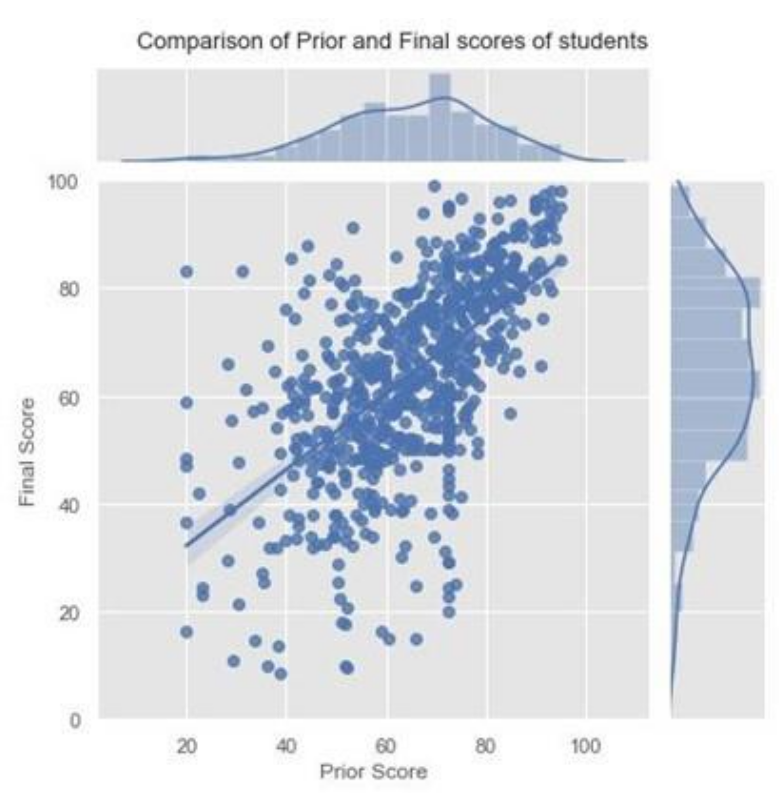
Students’ prior course grades had an impact on the students’ performance, as the prior course grade was linearly related to the final score (
Figure 1). Hence, the prior grades of the students along with the count of pass/fail for previous courses were measured.
Table 3 represents the various numerical and categorical features that were used for this study.
4.1. Predictive Modelling
The prediction was performed using classification algorithms that classify a given instance into a set of discrete categories; in our case, the pre-defined categories are at risk or not at risk. There is a wide range of algorithms supporting classification used throughout the literature. Choosing the optimal algorithm is difficult since they differ in numerous aspects, such as learning rate, robustness and the amount of data required for training, as well as their biases and behaviours on different datasets.
This study used the recently developed CatBoost [
23] algorithm for prediction tasks. CatBoost was chosen since it is flexible in its ability to work with both categorical and numeric features and is able to seamlessly function in the presence of missing values. A categorical feature is a feature that has a discrete set of values that are not essentially comparable with each other. In practice, categorical features are usually converted to numerical values before training, which can affect the efficiency and performance of the algorithm. However, CatBoost has been designed with the specific aim of handling categorical data. The ability to handle both categorical and missing data represents a considerable technical advantage over other algorithms, and a recent interdisciplinary review [
24] has found it to be competitive with other state-of-the-art algorithms.
CatBoost is a category boosting ensemble machine learning algorithm that uses the gradient boosting technique by combining a number of weak learners to form a strong learner. It does not use binary substitution of categorical values; instead, it performs a random permutation of the dataset and calculates the average label value for every object.
The combinations in CatBoost are created by combining all categorical features already used for previous splits in the current tree with all categorical features in the dataset. CatBoost thereby reduces overfitting, which leads to more generalised models [
23]. CatBoost uses ordered target statistics (Ordered TS) to tackle categorical features for a given value of the categorical feature, which means that the categorical feature is ranked before the sample is changed with the expectation of the original feature value. In addition, the priority and its weights are included. In this way, the categorical features are changed into numerical features, which effectively decreases the noise of low-frequency categorical features and improves the robustness of the algorithm [
25]. The performance of CatBoost was benchmarked against four other standard machine learning algorithms: Random Forest [
26], Naïve Bayes [
27], Logistic Regression [
28] and kNearest Neighbours [
29].
4.2. Machine Learning Procedure
The machine learning procedure used the hold-out method to perform the experiments where the order of occurrences of the training-test split was maintained. The experiments were implemented using Python [
30], which has built-in functions suitable for estimating and refining the results of predictions.
4.3. Model Evaluation
After designing the classification model, the next step is to evaluate the effectiveness of the model. This study used total accuracy, recall, precision and the F-measures derived from a confusion matrix [
31]. The total accuracy alone can be a misleading evaluation measure if the dataset is imbalanced because a model often favours learning and the prediction of a value of the most frequent class. This can give a misleading impression that the classifier has generalised better than it really has. In such circumstances, it is preferable to use the F-measure, which considers both precision and recall; an F-measure is the harmonic mean of precision (or positive predictive value) and recall (sensitivity) shown in Equation (2).
Precision is the measure of classifier’s exactness
Recall is the measure of the classifier’s correctness.
where
TP denotes TruePositive,
FP signifies FalsePositive,
FN represents FalseNegative, and
TN denotes TrueNegative.
Further, the AUC (Area Under the Curve)—ROC (Receiver Operating Characteristics) curve is a performance measurement for a classification problem at several threshold settings [
32]. ROC is a probability curve, and AUC signifies a measure of separability and is used for distinguishing between the class labels. AUC rates range from 0 to 1. The acceptable AUC range for a predictive model depends on the context. Typically, in most research areas, an AUC rate above 0.7 is preferred [
33]. In general, higher AUC scores indicate models of higher quality. The following equations are used for calculating AUC-ROC. In our study, we used the accuracy, F-measure and AUC as evaluation metrics. Our decision to use accuracy, F-measure and AUC as evaluation metrics is supported by a recent systematic literature review [
10] into the usage of predictive models in LA contexts.
4.4. Experimental Design
Our experimental design was devised in a manner that robustly evaluated the ability of our generic models to port across different courses and different deliveries of the same courses. We used a modified k-fold cross validation approach to evaluate our generic models. Given that our dataset is made up of seven different courses, and a total of 10 separate deliveries of those courses, we decided to train a model using nine course deliveries and test against the remaining hold-out course offering. We repeated this process 10 times with a different combination of training and hold-out courses in order to arrive at our final, aggregated evaluation scores for our models.
5. Results
The results from our evaluations in regard to portability of the generic (or course-agnostic) prediction model and feature selection approaches are described here.
5.1. Overall Performance Comparison of Classifiers
The generalisability of all the generic classifier models is shown in
Table 4, which records the aggregated model evaluation across all the hold-out datasets, together with the standard deviation over the 10 separate train/test executions. The best performing scores are in bold.
We can observe from the results that the F-measure scores range from 0.67 to 0.77, with CatBoost achieving the highest score. The variability across the different algorithms on all 10 datasets is similar, indicating that all algorithms generated generic models with a stable behaviour on all the courses.
The overall accuracy of all the algorithms has similarly ranged between 65% and 75%, with the result from CatBoost again clearly outperforming the other algorithms on these datasets. The accuracies of the bottom three algorithms, namely Naïve Bayes, Random Forest and Logistic Regression, did not exhibit significantly divergent accuracy results.
The AUC is a particularly effective measure of the effectiveness of the decision boundary generated by the classifiers tp separate out the two class labels representing at-risk and not at-risk students. These scores range from 0.71 to a very high score of 0.87, with CatBoost once more producing the best result and demonstrating that it has generated a classifier with the most effective decision boundary.
5.2. Classifier Performance Snapshots
The experimental results indicate that CatBoost is the most effective algorithm on these datasets and feature set, across the various standard algorithms considered in the study. Our attention now turns to examining the behaviour of the best performing algorithm on one of the hold-out datasets (Computer Applications and the Information Age—Semester 3). Our motivation was to analyse the ability of the algorithm to produce generic models that can identify at-risk students at early stages of a course so that in a practical setting, timely interventions can be initiated. To that end, we partitioned the dataset into 2, 4, 6 and 8 week intervals. We trained a CatBoost classifier on each snapshot/partition of the dataset in order to simulate a real-world scenario where only partial information is available at different stages and points in time of a course.
Figure 2 depicts the F-measure and AUC score for the CatBoost classifier on the hold-out dataset, depicting the metric scores at each of the 2, 4, 6 and 8 week snapshots in time. As expected, we observe that there is generally an improvement in the generalisability of the classifier as a course progresses and more data and a richer digital footprint are acquired for each student. However, the predictive accuracy as expressed by both AUC and the F-measure is still very high at an early 2-week mark, meaning that an accurate identification of at-risk students can already be made within two weeks of a course’s commencement, and that necessary interventions can be conducted as required in a timely fashion. Similar patterns were observed on the remaining nine hold-out datasets at the same snapshots in time.
5.3. Feature Importance
Feature importance analysis is an important aspect of machine learning, as it enables practitioners to understand what the key factors are that drive the predictions. In this analysis, we are able to quantify how much each feature of the data contributes to the model’s final prediction, thus introducing some measure of interpretability.
In this study, we used the Shapely Additive Explanations (SHAP) method [
34] for estimating feature importance and model behaviour. The SHAP method has the additional ability to depict how changing values of any given feature affect the final prediction. The SHAP method constructs an additive interpretation model based on the Shapley value. The Shapley value measures the marginal contribution of each feature to the entire cooperation. When a new feature is added to the model, the marginal contribution of the feature can be calculated with different feature permutations through SHAP. The feature importance ranking plot from the training data is shown in
Figure 3, representing the generic model from
Section 5.1.
In the SHAP feature importance graph seen in
Figure 3, each row signifies a feature. The features are arranged from the most important at the top to the least consequential at the bottom. The abscissa corresponds to the SHAP value (
Figure 4), which influences the final prediction. Every point in the plot denotes a sample, where red represents a higher feature value and blue represents a lower feature value. The vertical line on the plot, centred at 0 represents a neutral contribution towards a final prediction. As the points on the graph move further to the right on the
x-axis from this vertical line, the higher the positive contribution becomes towards the prediction of a student succeeding. The inverse is true for the strength of a contribution towards a prediction for an at-risk student as the values extend into the negatives on the
x-axis.
In our model, the assignment grades (both current and prior grades) played a vital part in prediction, which is unsurprising. We can observe from the graph that as the maximum grade for a student increased, the stronger this became as a predictor for positive outcomes. The reverse relationship also held; however, it was more acute, indicating that lower assignment grades had a stronger negative contribution than higher assignment grades for positive outcomes.
The above figure depicts the behaviours of the model at a global level. However, the SHAP method can also explain a given prediction for an individual student using a SHAP force plot (refer to
Figure 4). The force plot depicts the extent to which each of the most significant features is pushing a final prediction towards a negative or positive prediction. The ‘base value’ on the graph represents the mean prediction value, which can be regarded as a 50/50 point. Values to the right of the base value represent a final positive prediction and the inverse for the final values on the left. In the example below, we see that the assignment deviation score, the rolling assignment average score and the part-time study mode of a student most strongly influence the final prediction towards a positive prognosis for this specific student. Meanwhile, the age of the student has some influence towards a negative outcome prediction.
While feature importance shows what variables affect predictions the most, and force plots indicate the explainability of each model’s predictions for an individual student, it is also insightful to explore interaction effects between different features on the predicted outcome of a model. A dependence scatter plot seen in
Figure 5 demonstrates this. The
x-axis denotes the value of a target feature, and the y-axis is the SHAP value for that feature, which relates directly to the effect on the final prediction.
Figure 5a denotes that there is generally a positive correlation between LMS engagement scores and the assignment scores. Two noteworthy patterns emerge from
Figure 5a. First, we can see that students who score highly on the assignment scores but exhibit poor engagement levels with the LMS receive strongly negative outcome predictions by the model. We also see there is a threshold of 0.4 for the LMS engagement score, and those that score above this threshold are positively correlated with the model’s predictions for successful outcomes, which is amplified further for those with higher assignment scores.
Figure 5b considers the feature interaction of learner age and LMS engagement scores. Age of a student plays a significant role in the generated models. As the age of a student increases, the effect on the model predictions for positive outcomes becomes stronger. From approximately age 26 onwards, increases in the student age carry a stronger positive effect on model predictions for positive outcomes until age 40, from which point there do not appear to be any further increasing positive effects. Higher LMS engagement scores generally interact positively with age for successful outcomes. It is striking that those who are most at-risk are those in their early twenties with LMS engagement scores having no clear positive effect on prediction outcomes for this student demographic.
6. Discussion
The results have clearly indicated that generating viable generic models that are not tightly coupled to specific attributes of different courses is possible. The generic model has shown an effective average accuracy of around 75% across quite diverse courses. The diversity was seen in the fact that courses had varying numbers of assessments, differing distributions in their usage of the messaging Fora. Some courses used quizzes, books and various online learning resources, while others did not, or they differed greatly in their emphasis of their usage. The generic models were able to handle widely disparate courses, and despite them, produce useful predictive models even at earliest stages of a course’s delivery in order to permit timely interventions for at-risk students if necessary.
The 75% accuracy was stable across all the diverse courses, and it is comparable to predictive accuracies attained in published research. It could be argued that 75% accuracy may not be high enough to instil sufficient confidence in the models. However, one needs to keep in mind that the defined categories of ‘at-risk’ and ‘not at-risk’ are not black-and-white, clear-cut categories. These categories are moving targets and students are likely to fall into either category at different times of their study, or perhaps during different courses that they might be undertaking. Therefore, these categories embody many grey areas, and due to the lack of hard boundaries, the predictive accuracy can always be expected to be somewhat compromised when converting this complex problem describing a shifting continuum into a well-defined binary problem. One strategy to overcome this limitation is to instead focus on success prediction probabilities, which produce continuous valued outputs between 0 probability of success to 1, denoting complete confidence in successful outcomes. In addition to relying more on these outputs rather than on hard-thresholded binary categories, one can produce weekly probability predictions and monitor the change in the delta from one week to the next in order to generate deeper insights into the risk profile of a given student.
As for the superior performance of CatBoost over the other algorithms on these datasets, some of this can be attributed to the higher complexity of CatBoost over the other algorithms used in this study. CatBoost is a gradient boosting algorithm that makes it considerably more sophisticated than our benchmarking algorithms, capable of inducing more complex decision boundaries with some safeguards against overfitting. These internal mechanics undoubtedly contributed, but also the fact that it is able to seamlessly handle both missing and categorical data, which is not the case with the implementations of the other benchmarking algorithms. Both the missing data and categorical (mixed) data challenges often faced in the LA datasets, as well as the need to generate highly complex decision boundaries, do seem to indicate that this algorithm should form a part of the suite of algorithms that practitioners consider using in this problem domain.
7. Conclusions
The large volumes of LMS data related to teaching and learning interactions hold hidden knowledge about student learning behaviours. Educational data mining methods have the potential to extract behavioural patterns for the purpose of improving student academic performances via prediction models. Early prediction of students’ academic performance enables the identification of potential at-risk students, which provides opportunities for timely intervention to support them while at the same time encouraging those students who are not at risk to get more out of the course via data-driven recommendations and suggestions.
This study considered the problem of developing predictive models that have the capability to operate accurately across disparate courses in identifying at-risk students. Our study demonstrates how such generic and course-agnostic models can be developed in order to overcome the limitations of building multiple models, where each model is tightly coupled with the specific attributes of different courses. The portability of one model across multiple courses is useful because such generic models are less resource-intensive, easier to maintain, and less likely to overfit under certain conditions.
We formulated the machine learning problem as a binary-classification problem that labelled each student as either at risk of failing the course or otherwise. We demonstrated how features can be engineered that are not tightly coupled to the specifics of each course, and thus retain the property of being portable across all course types. Our experiments used Moodle log data, student demographic information and assignment scores from various semesters. Diverse courses were considered in order to robustly evaluate the degree to which our models were generic and portable.
The experiment was carried out using the commonly used Random Forest, Naïve Bayes, Logistic Regression and k-Nearest Neighbours algorithms, as well as the recently developed CatBoost algorithm. Across several performance metrics used in the experiments, the results indicated that the best performance was achieved using CatBoost on our datasets. CatBoost has capabilities in handling categorical features and missing data, while maintaining competitive generalisation abilities compared to current state-of-the-art algorithms. We performed a series of experiments in which we simulated the progression of a teaching semester, considering how early on within a given semester we could accurately identify an at-risk student. For this, our experiments considered data at regular intervals (i.e., at the end of week two, four, six and eight). Our results showed that from as early as two weeks into a course, our generic, course-agnostic model built using CatBoost was viable for identification of at-risk students and had the potential to reduce academic failure rates through early interventions.
Further, we observed that attributes related to assignment grades (current and prior grades) have a greater impact on model performance relative to other features. Also, students’ pre-enrolment data such as study mode, highest school qualification and English proficiency contributed positively to the model prediction. However, one of the most significant challenges in the space of predictive LA is to address how developed models can be effectively deployed across new and diverse courses. Our future work will expand the capabilities of our proposed model to an even broader set of courses.


