Improving Natural Language Person Description Search from Videos with Language Model Fine-Tuning and Approximate Nearest Neighbor

Abstract

Due to the ubiquitous nature of CCTV cameras that record continuously, there is a large amount of video data that are unstructured. Often, when these recordings have to be reviewed, it is to look for a specific person that fits a certain description. Currently, this is achieved by manual inspection of the videos, which is both time-consuming and labor-intensive. While person description search is not a new topic, in this work, we made two contributions. First, we improve upon the existing state-of-the-art by proposing unsupervised finetuning on the language model that forms a main part of the text branch of person description search models. This led to higher recall values on the standard dataset. The second contribution is that we engineered a complete pipeline from video files to fast searchable objects. Due to the use of an approximate nearest neighbor search and some model optimizations, a person description search can be performed such that the result is available immediately when deployed on a standard PC with no GPU, allowing an interactive search. We demonstrated the effectiveness of the system on new data and showed that most people in the videos can be successfully discovered by the search.

1. Introduction

Nowadays, in public places and even in private homes, there are many surveillance cameras. They record videos 24/7, producing large amounts of video data. If, for any reason, the videos have to be reviewed and the precise date and time are not available, then long segments of videos have to be reviewed manually. This is both labor-intensive and time-consuming. Typically, when surveillance is reviewed, one is looking for a specific person with a certain description, such as the clothes the person is wearing or the object they may have on their person. The problem of interest in this paper is: given a video clip and a natural language text description of a person, determine the timestamps in the video where people that match the description can be seen. One can then refer back to the original video at exactly the right moment and make further observations as needed, potentially saving a lot of effort and time.

In the literature, this task is known as a person description search. Since the task involves both a text description and cropped images of people in the video, it is a multimodal learning problem. Fundamentally, one seeks to produce embeddings of both image and text such that they are the same dimensions, and the embedding vectors are located near each other if the image–text pair is a match, i.e., they both are from the same person. On the other hand, they should be far apart if they are from different people. Joint embedding of image–text pairs generally involves a machine learning model with two branches, where one branch is responsible for producing the embedding of an image and the other one for the text. The embeddings are then aligned if they are a matched pair by a loss function that brings matched pairs together and pushes unmatched pairs away. Once trained, the model is used at an inference time as follows: a text description is written by a user, the embedding of the text is calculated, then it must be compared to the embeddings of the image of every unique person in the video that is being searched. The result of the search is the top-k closest image–text pairs. The user then reviews the images to see if any one of them actually matches the description or not, and if so, reviews the corresponding timestamp in the video. If no match is found, the description may need to be reworded, or another video can be tried.

Clearly, the search procedure outlined here is an iterative process that can involve many search queries. Moreover, for each query, the image embedding of every unique person in the video being searched must be calculated. This can take a significant amount of time if the video is long and/or there are a lot of people in the video. The problem is compounded by the fact that PCs that are used with surveillance cameras are generally low-cost ones that do not have the capability to perform heavy computation fast enough for a good user experience without long waits for every query.

In this paper, we propose a method that allows for an interactive search, i.e., the search result of each query is returned immediately. This is achieved by pre-indexing every video: for each video, we detect every unique person in the video and embed the image of each person. The image embedding vectors are then used to construct an approximate nearest neighbor (ANN) structure. The structure then acts as the “index” of the video. At inference time, one needs to embed only the query text, which can then be used in conjunction with the ANN structure to find the closest image in $log\left(n\right)$ time, where n is the number of unique people in the video. Moreover, we present a complete system for natural language person description search from videos in both English and Thai. For the English version, we experimented with different language models (LM) used as the embedding layers and demonstrated that using an LM that had been unsupervised—finetuned on the text of the target task before training—we were able to exceed the current state-of-the-art. For the Thai version, we tested the system in the field and demonstrated strong results on new test data that had not been used to train the model.

2. Related Works

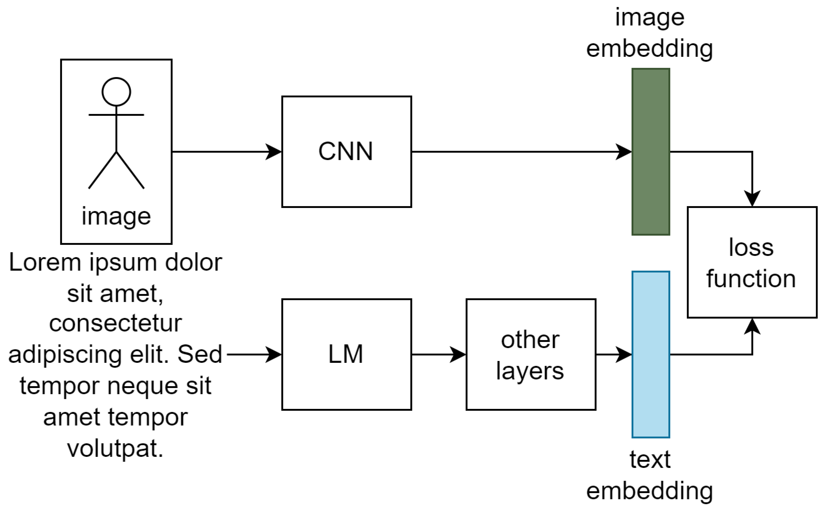
2.1. Joint Image-Text Embedding

Joint embedding of image–text pairs was considered as early as [1], where the visual branch consists of a convolutional neural network (CNN) [2]. The text branch was only compatible with single words, where the embeddings are obtained from a lookup table. The embedding of the image branch, which is in a higher dimension, goes into a linear transformation to make the dimensions match. The Hinge loss [3] was used to pull matched pairs together and push unmatched ones away. In [4], the image branch consists of the VGG [5] visual model, the text branch is a pipeline of first tokenizing the description into individual words, one-hot-encoding and concatenating them, and then passing through an LSTM [6] layer plus a single output gate at the back. The embeddings of both branches are then multiplied element-wise and summed. The resulting scalar is the similarity score of the image-text pair. In [7], a standard bi-directional LSTM was used as the first layer of the text branch, followed by max-pooling and fully connected layers in order to make the dimension of the embeddings of both branches the same. The image branch was given more attention in [8], and the structure consists of a bank of inception [9] modules. The output of which is multiplied back into the main flow of activation through the network at different layers to produce a kind of multi-level attention map. The strength at each level is modulated by a scaling weight, which is learned together with the model.

Joint image-text embedding can be categorized as global-level and local-level. Global-level methods consider the entire image of a person as a whole and do not have pre-built inductive bias toward any specific part of the image. Examples in this category are [10,11,12,13]. In [10], the local-level relationships between the image and text are left to be discovered by the latent-space co-attention mechanism. In [11], the authors used adversarial training, where the training objective includes a task to identify the original modality of an embedding. The work in [12] focused on hard-negative mining, a technique that is often used in image representation learning. Person description texts produced by different caption writers can have very different structures, and the work in [13] addressed this issue by performing image–text alignment prior to model training.

Methods that have an explicit inductive bias for local-level features are [14,15,16,17]. These works consider the local-level features explicitly either by having multiple models for different scales or by multi-level image–text alignment. In [14], the authors proposed two neural networks: one for what they called coarse-level features, and the other for fine-detail alignment between body parts and the noun phase in the text description. In [15], the image–text alignment was considered hierarchically at global–global, global–local, and local–local levels. Easy unmatched image–text pairs can be detected at the global–global level, while harder examples benefit from the local–local level alignment. The work in [16] separates features into three levels: whole body, top and bottom, and inside top/bottom plus footwear. Each level was embedded using a different neural network during training. In [17], the authors proposed a visual–textual attribute alignment that projects the feature of a person in image embedding space into subspaces of the text attributes. The loss values during training were calculated in each of the subspaces during training.

In addition to image–text joint features, other works focused on the loss function. In [18], a new component for the loss was introduced that considers each unique image–text pair as a distinct class and treats them as examples in a standard classification problem. This component of the loss was called the instance loss. In [19], a new loss function was proposed based on cross-modal projection matching [7]. The loss is the KL-divergence between the ideal distribution with 1.0 for a matched image–text pair and 0.0 everywhere else and the normalized projection between the image and text vector. The structure of the image branch was also considered in the work, and it was inspired by part-based features commonly used in the person re-identification [20] task. We focus our work on [19] as it is, at the time of writing, the state-of-the-art in person description searches according to [21] under the Text-based Person Retrieval on the CUHK-PEDES [22] benchmark.

2.2. Language Models in Person Description Search

A generic model structure for person description search is shown in Figure 1. The image branch is typically a visual model, such as some kind of CNN. The ResNet architecture [23] is a popular choice. The text branch nowadays is typically a large-scale LM based on the transformer architecture [24]. The BERT model [25] is a popular choice as it is the most well-known transformer-based LM. Since the text branch is basically a natural language processing (NLP) on its own, the structure of the text branch in Figure 1 follows the same development in NLP, where the transformer architecture now dominates. The key advantage of transformers is the attention mechanism, where the strength of the relationship between each pair of tokens in the text is explicitly weighted. This allows for an embedding of each word to not be isolated like in traditional word embedding but to consider the context of the entire text. The overall embedding of the text produced by a transformer-based LM is a better representation of the text, which benefits downstream tasks where the embedding is used.

Transformer-based models are usually trained in a two-stage manner: pretraining followed by finetuning. Large language models are never trained from randomly initialized weights directly on the target supervised task; instead, they are first pre-trained. Pretraining consists of training the model from randomly initialized weights, but the training task is unsupervised. In unsupervised pretraining, the task is either to predict the next word given the words that came before it or to predict words that had been masked out in a sentence. The first is called autoregressive LM, and the second one is called the mask language model (MLM). It can be seen that there is no labeling needed as the correct answer is dictated by the data itself. Data for this step are usually large open-domain text, such as the book corpus [26]. Once the pretraining step is complete, the weights are saved from being used as initial weights for the finetuning phase. Finetuning is training the model initialized by the pretraining weights on a supervised learning task normally. Optionally, one can perform an extra step between pretraining and finetuning called LM-finetuning, where the LM is trained using the same loss as in pretraining but on the text of the finetuning task, i.e., unsupervised MLM training but using texts for the person description search. This step is beneficial if the target task has a specific language structure that may not always be present in the pretraining data.

2.3. Loss for Image-Text Matching

The loss function used in one of the most recent works on person description search is cross-modal projection matching (CMPM). This loss is different from other representation learning losses, such as the aforementioned hinge loss or the triplet loss [27], in that it makes use of information-theoretic criteria. Instead of viewing the embedding of both branches as just vectors, CMPM formally defines these vectors as samples from unknown probability distribution. Specifically, a training batch is defined as ${\left\{(v_i^I,v_j^T),y_{i,j}\right\}}_{j=1}^N$ where I and T indicate image and text modality, $v_i$ and $v_j$ are embedding vectors and $y_{i,j}=1$ if $v_i^I$, N is the batch size and $v_j^T$ are from the same person and zero if otherwise. The probability that $v_i^I$ and $v_j^T$ are a matched pair is defined using the softmax function ((3) from [19])

$$p_{i,j}=\frac{exp\left({\left(v_i^I\right)}^{\top }{\overline{v}}_j^T\right)}{{\sum }_{k=1}^{N}exp\left({\left(v_i^I\right)}^{\top }{\overline{v}}_k^T\right)}$$

(1)

where ${\overline{v}}_j^T$ is the normalized text embedding vector. The inner product is the projection of $v_i^I$ onto ${\overline{v}}_j^T$. For a matched pair, ideally these two are the same vector, and the probability becomes 1. For an unmatched pair, ideally the vectors are perpendicular and the probability is zero. The core idea of CMPM loss is that one defines the ideal distribution $q_{i,j}$ as

$$q_{i,j}=\frac{y_{i,j}}{{\sum }_{k=1}^N{y}_{i,k}}$$

(2)

where $y_{i,j}$ is the indicator function as defined above. This distribution is 1 where $i,j$ forms a matched pair and zero otherwise. One then tries to minimize the distance between $y_{i,j}$ to the ideal distribution $q_{i,j}$ by minimizing the KL-divergence between them

$$L_{I2T}=\frac{1}{N}\sum _{i=1}^N\sum _{j=1}^N{p}_{i,j}log\left(\frac{p_{i,j}}{q_{i,j}+ϵ}\right)$$

(3)

where $ϵ$ is a small constant for numerical stability. The $I2T$ indicates that this is the loss for the image to text direction. Since the KL-divergence is not symmetric, the loss in the other direction can be similarly defined, and the final loss is the sum between the two. In [19], this loss is computed using not only the final embedding of each branch but also the intermediate outputs of each layer as well. The ultimate loss is the weighted sum of the loss at each layer.

2.4. Approximated Nearest Neighbor Search

At the search time, a user would supply the text description. Finding the matched image involves calculating the embedding vector of an image and then the inner product in (1). Repeat for all images and then rank the results in decreasing order of inner product value. Typically, the top-k most similar images are returned to the user. The clear disadvantage of this direct approach is that the number of image embedding vectors that had to be calculated is the same as the number of people in the video. If it is collected from a crowded location, even a relatively short video can contain hundreds of people. Each additional person requires one extra forward pass through the image branch of the model, which can be quite slow if the PC is not equipped with a discrete GPU.

This issue can be overcome by using approximated nearest neighbors and preprocessing each video before search time. Assuming that each person in the video had been detected, the image of each person is passed through the image branch, the set of image embedding vectors obtained can then be used to build an ANN index. The principle of ANN [28] is: given a set of vectors, repeatedly generate a random hyperplane to partition the space. Each added hyperplane exponentially increases the number of partitions in the space of increasingly smaller size. This process is repeated until each partition has only a single vector, as illustrated in Figure 2. In terms of data structure, each hyperplane corresponds to a node in a binary tree, where the leaves of this tree are the final partitions. At a search time, given a query vector, one traverses this tree from root, taking the direction at each node according to which side of the hyperplane the query vector lies on, until one arrives at a leaf. The vector that corresponds to that partition is the nearest neighbor of the query vector. Since the height of the tree is $log\left(n\right)$ on average and, in practice, multiple trees are generated for robustness, the complexity of the search operation is $Plog\left(n\right)$ where P is the number of trees—a hyperparameter that can be chosen as a tradeoff between speed vs. accuracy.

2.5. Object Detection and Tracking

The first step for indexing a video file is to detect and track each person in the video. Object detection is a well-studied problem in computer vision. The task is to locate each object in an image or a video frame and determine the coordinate of a tight bounding box around each object of interest, i.e., people. From the bounding box coordinate, the objects can be cropped out for object-specific further processing. In other applications, object detection can be used to count the number of objects of each type in an image for understanding a scene. Modern object detection methods use CNN as the backbone and can be roughly categorized into two groups: multi-pass methods [29] and single pass methods [30,31]. As the name implies, single pass methods are faster in terms of frames per second because only one pass through the model is needed for each frame. Since in this work we are concerned with potentially very long videos, we focus on the single pass method. Out of the two families of single pass detectors, the Yolo family is more widely used. In the original version of Yolo, an image is divided into a grid of seven-by-seven cells. Each cell is responsible for detecting at most two objects whose centroid’s coordinates fall within the cell. The target output of the model is a 3D array of shape seven by seven by L. The class label and bounding box coordinate of each object (or two objects) is encoded in the one-by-L vector “tube”. Furthermore, part of the tube is the probability that this cell has an object, set to one for cells that actually contain an object and zero for cells that do not. The loss function is a weighted sum of softmax loss for object type classification, the mean square error for the bounding box coordinates, and the “objectness” probability. Later versions offered improvements such as normalizing the bounding box coordinate, anchor boxes, increased input resolution and speed optimization.

Object detection is not enough to prepare a video for a fast person description search. This is because the videos were recorded at 24 to 30 fps. Thus, if one were to use object detection alone, one would get a large number of images for each person. This is not good for two reasons: first, it increases the number of images that must be embedded when a video is being indexed; second, it floods the search space with many vectors that do not contribute any new information. Ideally, one would like to have only a single image for each person in the video. Object tracking [20] allows us to track individual objects through many video frames. It works on top of object detection, where the detection results of consecutive frames are compared and bounding boxes that are close in size and location across frames are potentially the same person. This is checked using person re-identification [32], a task that shares some similarities with the person description search. For person re-identification, the goal is to build a robust embedding of people such that images of the same person that are different because of lighting, posture and camera angle can be identified as such. Typically, a model for this task has two branches, like the person description search, but the main difference is that both of these branches are identical image models. When the two inputs are from the same person, the model should output a one, and when they are from different people, output a zero. Person re-identification draws from a large body of literature on representation learning [33] that seeks to learn robust vector representation of objects. This is commonly achieved by training a model to distinguish between pairs of images where one is the original and the other is randomly a heavily augmented version of the same object or a different object entirely.

Since neither object detection nor tracking is the main focus of this work, we used off-the-shelf implementation of these tools without any modification. They form part of the pipeline to prepare a video for fast person description search.

3. Methods

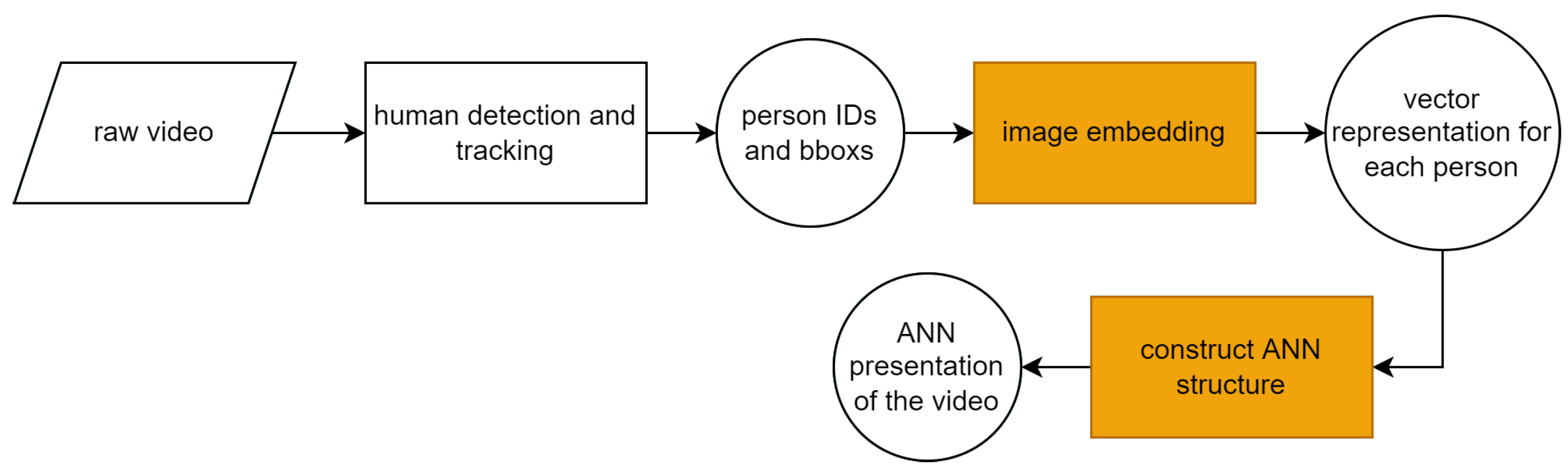
3.1. Video Indexing Pipeline

The proposed pipeline is shown in Figure 3. The rectangles represent processes, while the circles represent data objects. Given a video, the first step of the pipeline is to detect and track the people in the video. We used the implementation of [34] for the detector and tracker. The tracking result is checked if any bounding box has a side smaller than S pixels long (see Algorithm 1), and if so, they are removed. The remaining bounding boxes are then sorted by object IDs, which are assigned consecutively by the tracking engine, after which the bounding boxes, which have the same object ID, are then sorted by the bounding box sizes. The bounding box that has the median size is chosen to be the representative image of the person. This choice was made to avoid bounding boxes that are too small (the person is too far from the camera) or too large (the person is too close to the camera such that their entire body does not fit in the camera frame). The decision to choose the bounding box with the median size was made after experimenting with other criteria such as bounding box size and aspect ratio. Unfortunately, these criteria are not robust to the posture of a person, such as sitting down or riding a bicycle, or the recording resolution. Algorithm 1 is the process of detecting unique persons from the video and choosing the best bounding box to represent each person.

After the image of each person in the video is obtained, the text branch of the model is embedded. We use the same model structure as in [19]. The output is the image embedding vector of each person. Finally, the ANN structure is constructed from all the vectors. We used the implementation of [35]. The ANN object is effectively the index of the entire video. The bounding box images are kept and named <person id>_<frame number>. The <frame number> is important as it allows one to convert back to the exact time in the video that this image came from. The process of building an ANN object from a video is give in Algorithm 2. The process in the pipeline is repeated for each video that is to be made searchable. In terms of the speed of the pipeline, for a video with 1080p resolution, the detection and tracking take approximately 50% of the length of the video, while the embedding and construction of the ANN take less than one minute on a PC with a GPU. The indexing time, however, is not really a limitation, as for an actual deployment, the detection and tracking can be performed on the live stream as the video is being recorded. Real-time tracking at 24–30 fps and 1080p is easily possible using Yolo and a PC with a low-end GPU. Finally, the search progress is given in Algorithm 3. At the search time, only the text description needs to be embedded, which only requires a single forward pass through the model.

Algorithm 1 Tracking and Bounding Box Filtering

Require: path                         ▷ The path to a video file to be indexed.   1: doTracking(path) ▷ Run YOLOv5 tracking [34] on the video file, the output trackResult is a text file.   2: initialize Table (Pandas Dataframe) with columns: frameID, personID, bbox, area   3: for each line in trackResult do                 ▷ Each line describes a detected bbox.   4:     if width >= S and height >= S then         ▷ S is a threshold set according to video resolution   5:         append frameID, personID, bbox, area to Table   6:     end if   7: end for   8: sort Table by personID and then by area   9: for each group of rows in Table with the same personID do   10:     saveFrameID = medianRow.frameID ▷ medianRow is row with median area among this personID.   11:     crop from the saveFrameIDth frame in the video file using medianRow.bbox   12:     save the cropped image as img_<videoName>_<personID>_<frameID>   13: end for

Algorithm 2 Building ANN Structure for Fast Person Description Search

Require: path ▷ Path to a folder containing all the bbox images from a video obtained by Algorithm 1. Require: model     ▷ Loaded ONNX model for the person description search model.   1: initialize ANN object [35] with parameters space = ‘ip’ and dim = 2048   2: for each image in path do   3:     read image from disk and apply preprocessing   4:     imgEmbed, textEmbed = model(image, text)   ▷ Run forward pass on the model. imgEmbed is the embedding of the input (person) image. The text input which is not used can be set to all padding character.   5:     add imgEmbed to ANN ▷ Note that the image embeddings are added in the same order as personID.   6: end for   7: save ANN to a Python pickle file with the same name as the video ▷ The pickle file is the “index” of the current video.

Algorithm 3 Searching The ANN Structure

Require: videoName   ▷ The filename of the video (indexed by Algorithms 1 and 2) to search. Require: description             ▷ The description of the person to search. Require: model    ▷ Loaded ONNX model for the person description search model.   1: ANN = Load the ANN model (saved pickle file from Algorithm 2) of this video.   2: imgEmbed, textEmbed = model(image, description) ▷ The image input can simply be set to all-black image.   3: mostSimilarIndices = ANN.knn_query(textEmbed, top_k=K)  ▷ mostSimilarIndices holds personID of the top-K most matched to the description.

3.2. LM-Finetuning and Model Training

We obtained the CUHK-PEDES dataset [22] courtesy of the authors. The dataset consists of image–description pairs, where one image is paired with at least 2 or more descriptions. We performed LM-finetuning for both English and Thai. For English, the data were used as is. For Thai, it was first translated using an en-th machine translation model. We experimented with two types of models as the LM: the aforementioned BERT, and RoBERTa [36]. Structurally, RoBERTa is identical to BERT. It is pretrained with more data, and one component of the pretraining loss function used in BERT is removed. The loss function used to pretrain BERT is MLM prediction loss + next sentence prediction (NSP) loss. The MLM loss is from predicting the masked words in a sentence. For the NSP loss, the model is fed two sentences A and B and asked to predict whether they are actually consecutive sentences or if B is an unrelated sentence. RoBERTa does not make use of NSP loss and the authors argued that NSP is actually detrimental to performance. While we cannot determine if this statement is actually true or not, the lack of NSP is actually an advantage for us for two reasons. The first is that some person descriptions are only one sentence long, making it impossible to calculate NSP loss. The second reason is specific only for Thai, which has no sentence boundary marker and loose grammatical structure. Sentence boundaries are quite ambiguous in Thai, even for a human reader. This makes the NSP loss impractical. For Thai, there is a version of the RoBERTa model pretrained on Thai text called WangchanBERTa [37] and also RoBERTa pretrained on 100 languages known as xlm-roberta [38]. Each LM was finetuned with just MLM loss (no NSP loss even for BERT) with the hyperparameters summarized in

Table 1. The hyperparameters for LM-finetuning.

Hyperparameter	Value
batch size	32
learning rate	$2.5\times {10}^{-5}$
MLM mask probability	5%
maximum text length	64 (subword) tokens
weight decay	0.001
warmup steps	1400
half precision (FP16)	true
train epochs	100
early stopping patient	10 epoch
optimizer	Adam

. We used the Hugging Face [39] implementation of the LMs, and the initial pretrained weights were obtained from the Hugging Face’s Model Repository.

For the supervised model training, we trained the TIPCB model using the same data splits as in the original paper [19]. The important training hyperparameters are summarized in

Table 2. The hyperparameters for supervised training.

Hyperparameter	Value
batch size	32
learning rate	$2.5\times {10}^{-5}$
Maximum text length (tokens)	64
Weight decay	$4.0\times {10}^{-5}$
Number of epochs	80
Learning rate reduction epoch	40
Learning rate reduction factor	10
Warmup epochs	10
optimizer	Adam

. We reimplemented the training code in the Pytorch Lightning [40] framework, which allows easy use of half precision (FP16) mode, resulting in significantly shorter training time. To allow for direct comparison with the original work, besides swapping the LM part of the model and utilizing FP16, there was no change made to the hyperparameters, the model (except increasing the hidden layer size to match when larger versions of the LMs were used), or the data pipeline.

3.3. ANN Construction

Once the model is trained, it can be used as part of the pipeline in Figure 3 at the image embedding step. As this step has to be performed for each video to be indexed, it is desirable to make the model run as fast as possible. We convert the pytorch checkpoint of the best epoch (the epoch with the best top 1 recall) into ONNX format [41]. The ONNX format is proposed to be a common format for storing deep neural networks that is compatible with all major deep learning frameworks and all backends (x86, ARM, CUDA). Inference with ONNX also benefits from optimizations such as weight quantization, reduced weight precision, and model pruning, etc. Another benefit of using ONNX is cross-platform compatibility and the independence of the original deep learning framework originally used to train the model.

The trained model was converted to ONNX. The input batch size was chosen to be dynamic (inferred during inference time), the input image size was fixed at 128 × 384 pixels, for the text branch the input length was fixed at 64. The ONNX opset version was 11. The exported ONNX model was used to embed all images from each video, and the batch size for embedding was 32. Once the image embedding vectors of a video are calculated, we construct the ANN structure using the hnswlib library [42]. The parameter for ANN construction was chosen as follows: the type of distance was the inner product to match with (1). The number of trees $ef$ was 200, and the number of bi-directional splits for each vector added M was 48. The resulting ANN object was serialized to a Python pickle file for deployment. Each video that is indexed generates one pickle used for deployment.

4. Results

4.1. The Impact of LM-Finetuning

First, we present the result that LM-finetuning has on the performance of the supervised model.

Table 3. The top-k recall value of the supervised model trained with various LM configurations as the initial weight. For the English version, we considered BERT-base (≈120 M parameters), BERT-large (≈300 M parameters), RoBERTa-base and RoBERTa-large. For Thai, we considered WanchangBERTa (it does not have a large version), xlm-roberta-base and xlm-roberta-large. For each LM type, both LM-finetuned and not finetuned were considered. It can be seen for every type that LM-finetuning leads to improved recall for all values of k except for BERT-large vs. BERT-base. The best configuration for English was a finetuned RoBERTa-base with 0.6451, 0.8303 and 0.8919 top 1, 5, and 10, respectively. The top-1 value is higher than 0.6363 reported in [19]. For Thai, the best configuration was finetuned xlm-roberta-base.

Language	Model	LM-Finetune	Top-1	Top-5	Top-10
en	BERT-base	n	0.6314	0.8266	0.8890
en	BERT-base	y	0.6424	0.8297	0.8930
en	BERT-large	n	0.6399	0.8332	0.8933
en	BERT-large	y	0.6354	0.8327	0.8862
en	RoBERTa-base	n	0.6324	0.8294	0.8901
en	RoBERTa-base	y	0.6451	0.8303	0.8919
en	RoBERTa-large	n	0.6319	0.8221	0.8874
en	RoBERTa-large	y	0.6429	0.8285	0.8905
th	WangchanBERTa	n	0.1690	0.2935	0.3578
th	WangchanBERTa	y	0.5737	0.7771	0.8452
th	xlm-roberta-base	n	0.5566	0.7720	0.8470
th	xlm-roberta-base	y	0.5745	0.7794	0.8507
th	xlm-roberta-large	n	0.5564	0.7668	0.8436
th	xlm-roberta-large	y	0.5695	0.7802	0.8468

shows the top-k recall value of the supervised model trained with various LM configurations as the initial weight. It can be seen that for every type that LM-finetuning leads to improved recall for all values of k, except for BERT-large vs. BERT-base, where the reason may be because of the lack of the NSP loss that BERT originally used. The difference between finetuning and not finetuning is largest for WanchanBERTa. The best configuration for English was the finetuned RoBERTa-base with top-1, top-5 and top-10 recall values of 0.6451, 0.8303, and 0.8919, respectively. All of the recall values are higher than those reported in [19], which are 0.6363, 0.8281, and 0.8901, respectively. Our recall values are also higher than those reported in [43] of 0.6408, 0.8173, and 0.8819, respectively. Note that the top-1 recall of [43] is higher than that in [19], but ours is the highest for all top-k values. The result demonstrates the benefit that LM-finetuning has on the person description search model. The top-1 value is higher than 0.6363 reported in [19]. For Thai, the best configuration was the finetuned xlm-roberta-base. However, for deployment, we went with WangchanBERTa instead, as xlm-roberta is a cross-language model with a large vocabulary and, therefore, a large embedding layer that requires more computation to run. The rest of the results shown in this section are with respect to the LM-finetuned WanchanBERTa configuration.

4.2. System for Person Description Search

Next, we present the person description search results on new data with fast search enabled by pre-embedding the images and using ANN. The test videos were recorded at Thammasat University Rangsit campus. The camera used was a GoPro Hero 10. The recording resolution was 1080p, and the frame rate was 30 fps. The camera was mounted on a pole at a height of around 3 m. Each video was processed, as described in Figure 3. The model and processed videos are deployed on a cloud virtual machine with 2 CPU cores, 4 GB of RAM and no GPU. Due to the use of ANN, only one forward pass through the text branch of the model is needed during the search. The optimizations made by the ONNX format enable this forward pass to run very fast. Upon clicking search, the results are available immediately in about 1 s. In contrast, for the same video, there are 187 images that must be processed by the model if one were to naively deploy the model. The time that it takes to perform this calculation is longer than the default HTTP request timeout using NGINX as the web server of 60 s. The immediate search allows one to use the system interactively and try different phasing for the queries and/or different videos quickly, leading to a better user experience.

Figure 4 shows a screenshot of the web interface for fast person description search. For demonstration purposes, only two video files are shown, but in reality, there is no limit on the number of video files that can be made available for search. Figure 5 shows the search result of the query “short sleeve grey t-shirt grey short grey pants sandals bag” (Thai literal translation). It can be seen that the top 2 matches are the correct person that fits the description. For each search result, the time in the original video is shown so that users can quickly cross-check and, if necessary, observe the person more. Figure 6 shows the video file at the same time as the top result in Figure 5, and it can be seen that it is the correct time that matches the search result.

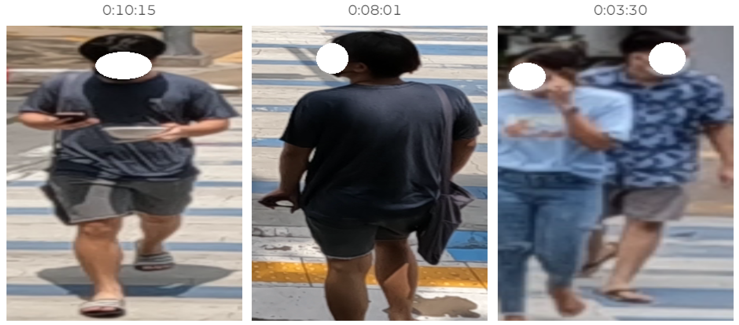
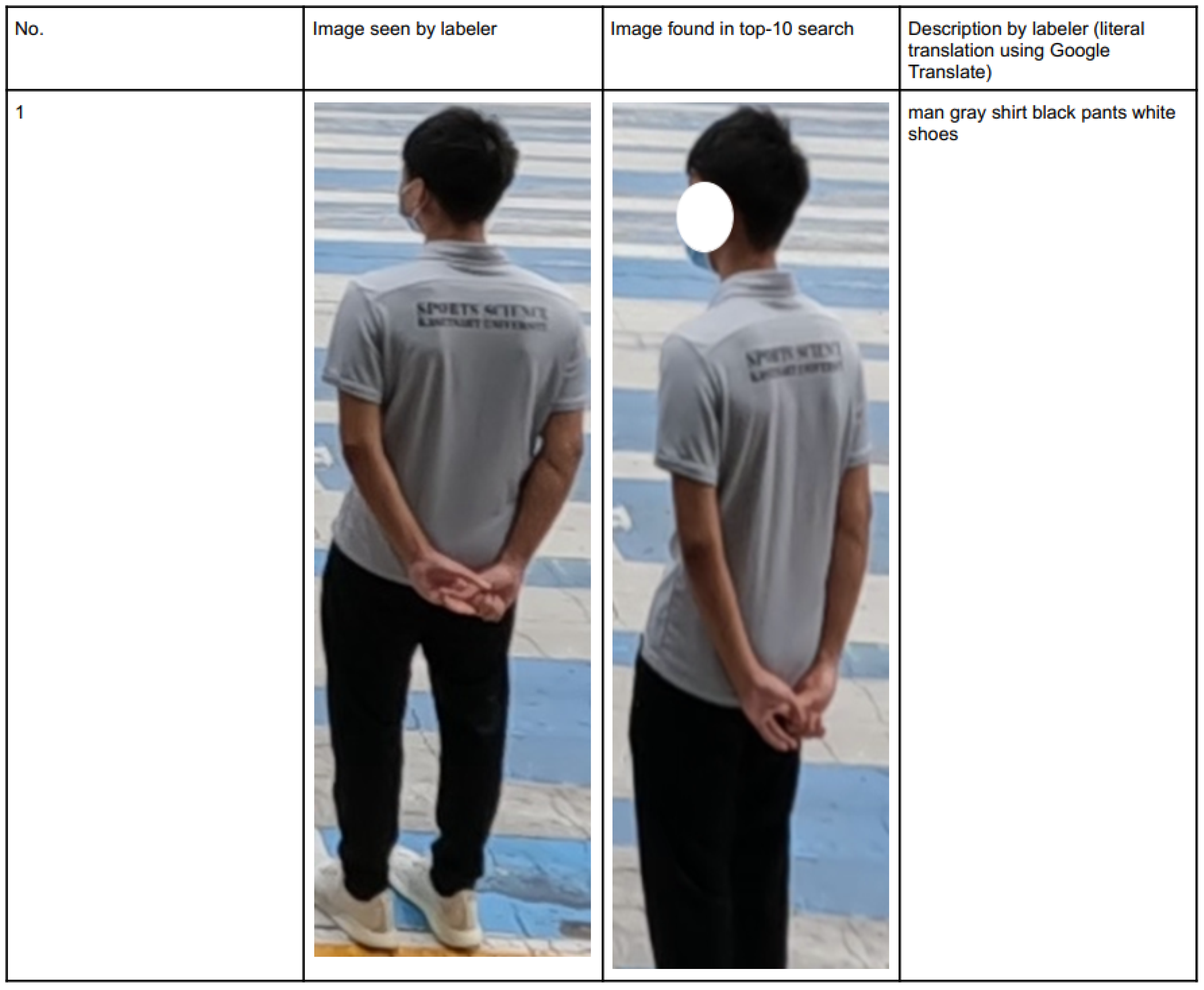
4.3. Search Result on Unseen Data

Part of this work is an ongoing process of building a new dataset for a person description search. For each video obtained, as described in the previous section, we performed detection and tracking to get a cropped image of each person. The corresponding text description for each is written by multiple labelers. For each image, we plan to have at least two descriptions that were written by different people. In order to enable multiple people to work concurrently and keep the data at a central location, we create a separate web interface for the labelers to use. Each labeler’s descriptions are kept separate from the others by assigning each labeler to a separate collection in the database.

We used some of the newly labeled data to simulate actual use and test the effectiveness of the proposed search system. For each image that the labelers see, we take the description written by one labeler and then run it through the system to check if the same person can be found in the top-10 result. Whether the same person had been found was checked by manual inspection of the returned images. This was performed on the images of 50 different people. Figure 7 shows one example of the results. The full results can be found in the supplementary data. Out of 50 searches, 46 were successful, which gives a top-10 recall value of 0.92.

4.4. Comparison of Search Speeds

We compared the search speeds between our method and the direct method. The direct method consists of calculating and embedding the search query on each image of a person (only a single image for each person) found in a video. Then, the nearest neighbor is calcuated exactly. The results for three different videos are summarized in

Table 4. Comparison between the search speed of the direct method and our method. In all cases, the direct method is unacceptably slow. When there are a large number of people in a video, the search time is so slow that it leads to an http request timeout, such as in the case of video 1.

Video	Number of People	Direct Method	Our Method
1	383	timeout (>1 min)	<1 s
2	103	24 s	<1 s
3	207	47 s	<1 s

.

4.5. Limitations

While working quite well, the system has some limitations. The first limitation is that a video must go through object detection and tracking and then the building of the ANN object. In our current implementation, object detection and tracking take roughly half the length of a video itself. In future work, we plan to work around this issue by performing detection and tracking as the video is being recorded, so that this step in the pipeline is no longer the bottleneck. The second limitation is of the person description model itself. To showcase this limitation, consider the target person shown in Figure 8, and the search result using the description “white t-shirt women jeans” (direct Google Translated) shown in Figure 9. It can be seen that the system was able to find people who generally fit the description, i.e., wearing a white t-shirt and/or jeans, but it was unable to find the correct person. Furthermore, the description was short as the target person does not have any other distinctive features: her shoes are not clearly visible, and she is not holding anything on her person. Person description search faces a challenge when there are a lot of people with similar clothes, for example, uniforms, or a lack of features that can easily be described in words. One possible way to tackle this problem is to take advantage of face mask color/styles (she is wearing a pink surgical mask), but currently, the model does not know of face masks because it was trained with data collected before 2020. Another limitation is that the search is essentially a “closeness” measure and not a hard yes/no; thus, if a man is wearing a white t-shirt, he will be close to the description “white t-shirt women jeans” even when the gender is wrong. This is another challenge that we defer for further research.

5. Conclusions

In this paper, we present a real-time natural language person description search from videos with two main contributions. The first contribution is that we propose finetuning of the language models that are part of the text branch of modern person description search models on the target task’s data before supervised training. We demonstrated that doing so led to improved recall across all top k values and across all language model types. The second contribution is that we engineered a system that spanned the entire process from raw video to fast searchable objects. The system is built for Thai text, but changing it to any other language can be easily achieved by swapping out the language model and retraining. We demonstrated the effectiveness of the system by searching new unseen-in-training-data videos with query descriptions written by a labeler with no knowledge of how the model works and found that for the top-10 results, most people in the videos can be correctly discovered from the search. Moreover, the search is very fast, and the result is available immediately, allowing the system to be used interactively. For future work, we plan to optimize the pipeline further so that the detection and tracking part can be run live as the video is being recorded to amortize the computational cost and make the entire pipeline able to run on a regular PC with no GPU. Another improvement is to take advantage of new features such as face masks and improve the ability to differentiate between genders.

References

1. Frome, A.; Corrado, G.S.; Shlens, J.; Bengio, S.; Dean, J.; Ranzato, M.; Mikolov, T. Devise: A deep visual-semantic embedding model. Adv. Neural Inf. Process. Syst. 2013, 26, 2121–2129. [Google Scholar]
2. LeCun, Y.; Boser, B.; Denker, J.S.; Henderson, D.; Howard, R.E.; Hubbard, W.; Jackel, L.D. Backpropagation applied to handwritten zip code recognition. Neural Comput. 1989, 1, 541–551. [Google Scholar] [CrossRef]
3. Rosasco, L.; De Vito, E.; Caponnetto, A.; Piana, M.; Verri, A. Are loss functions all the same? Neural Comput. 2004, 16, 1063–1076. [Google Scholar] [CrossRef] [PubMed] [Green Version]
4. Li, S.; Xiao, T.; Li, H.; Zhou, B.; Yue, D.; Wang, X. Person search with natural language description. In Proceedings of the IEEE Conference on Computer Vision and Pattern Recognition, Honolulu, HI, USA, 21–26 July 2017; pp. 1970–1979. [Google Scholar]
5. Simonyan, K.; Zisserman, A. Very deep convolutional networks for large-scale image recognition. arXiv 2014, arXiv:1409.1556. [Google Scholar]
6. Hochreiter, S.; Schmidhuber, J. Long short-term memory. Neural Comput. 1997, 9, 1735–1780. [Google Scholar] [CrossRef] [PubMed]
7. Zhang, Y.; Lu, H. Deep cross-modal projection learning for image-text matching. In Proceedings of the European Conference on Computer Vision (ECCV), Munich, Germany, 8–14 September 2018; pp. 686–701. [Google Scholar]
8. Liu, X.; Zhao, H.; Tian, M.; Sheng, L.; Shao, J.; Yi, S.; Yan, J.; Wang, X. Hydraplus-net: Attentive deep features for pedestrian analysis. In Proceedings of the IEEE International Conference on Computer Vision, Venice, Italy, 22–29 October 2017; pp. 350–359. [Google Scholar]
9. Szegedy, C.; Vanhoucke, V.; Ioffe, S.; Shlens, J.; Wojna, Z. Rethinking the inception architecture for computer vision. In Proceedings of the IEEE Conference on Computer Vision and Pattern Recognition, Las Vegas, NV, USA, 27–30 June 2016; pp. 2818–2826. [Google Scholar]
10. Li, S.; Xiao, T.; Li, H.; Yang, W.; Wang, X. Identity-aware textual-visual matching with latent co-attention. In Proceedings of the IEEE International Conference on Computer Vision, Venice, Italy, 22–29 October 2017; pp. 1890–1899. [Google Scholar]
11. Sarafianos, N.; Xu, X.; Kakadiaris, I.A. Adversarial representation learning for text-to-image matching. In Proceedings of the IEEE/CVF International Conference on Computer Vision, Seoul, Korea, 27 October–2 November; pp. 5814–5824.
12. Ge, J.; Gao, G.; Liu, Z. Visual-textual association with hardest and semi-hard negative pairs mining for person search. arXiv 2019, arXiv:1912.03083. [Google Scholar]
13. Niu, K.; Huang, Y.; Wang, L. Fusing two directions in cross-domain adaption for real life person search by language. In Proceedings of the IEEE/CVF International Conference on Computer Vision Workshops, Seoul, Korea, 27–28 October 2019. [Google Scholar]
14. Jing, Y.; Si, C.; Wang, J.; Wang, W.; Wang, L.; Tan, T. Pose-guided multi-granularity attention network for text-based person search. In Proceedings of the AAAI Conference on Artificial Intelligence, New York, NY, USA, 7–12 February 2020; Volume 34, pp. 11189–11196. [Google Scholar]
15. Niu, K.; Huang, Y.; Ouyang, W.; Wang, L. Improving description-based person re-identification by multi-granularity image-text alignments. IEEE Trans. Image Process. 2020, 29, 5542–5556. [Google Scholar] [CrossRef] [PubMed] [Green Version]
16. Gao, C.; Cai, G.; Jiang, X.; Zheng, F.; Zhang, J.; Gong, Y.; Peng, P.; Guo, X.; Sun, X. Contextual non-local alignment over full-scale representation for text-based person search. arXiv 2021, arXiv:2101.03036. [Google Scholar]
17. Wang, Z.; Fang, Z.; Wang, J.; Yang, Y. Vitaa: Visual-textual attributes alignment in person search by natural language. In Proceedings of the European Conference on Computer Vision, Glasgow, UK, 23–28 August 2020; pp. 402–420. [Google Scholar]
18. Zheng, Z.; Zheng, L.; Garrett, M.; Yang, Y.; Xu, M.; Shen, Y.D. Dual-path convolutional image-text embeddings with instance loss. ACM Trans. Multimed. Comput. Commun. Appl. (TOMM) 2020, 16, 1–23. [Google Scholar] [CrossRef]
19. Chen, Y.; Zhang, G.; Lu, Y.; Wang, Z.; Zheng, Y. TIPCB: A simple but effective part-based convolutional baseline for text-based person search. Neurocomputing 2022, 494, 171–181. [Google Scholar] [CrossRef]
20. Wojke, N.; Bewley, A.; Paulus, D. Simple online and realtime tracking with a deep association metric. In Proceedings of the 2017 IEEE International Conference on Image Processing (ICIP), Beijing, China, 17–20 September 2017; pp. 3645–3649. [Google Scholar]
21. The Latest in Machine Learning|Papers with Code. Available online: https://paperswithcode.com (accessed on 25 October 2022).
22. Xiao, T.; Li, S.; Wang, B.; Lin, L.; Wang, X. End-to-end deep learning for person search. arXiv 2016, arXiv:1604.01850. [Google Scholar]
23. He, K.; Zhang, X.; Ren, S.; Sun, J. Deep residual learning for image recognition. In Proceedings of the IEEE Conference on Computer Vision and Pattern Recognition, Las Vegas, NV, USA, 27–30 June 2016; pp. 770–778. [Google Scholar]
24. Vaswani, A.; Shazeer, N.; Parmar, N.; Uszkoreit, J.; Jones, L.; Gomez, A.N.; Kaiser, Ł.; Polosukhin, I. Attention is all you need. Adv. Neural Inf. Process. Syst. 2017, 30, 6000–6010. [Google Scholar]
25. Devlin, J.; Chang, M.W.; Lee, K.; Toutanova, K. Bert: Pre-training of deep bidirectional transformers for language understanding. arXiv 2018, arXiv:1810.04805. [Google Scholar]
26. Zhu, Y.; Kiros, R.; Zemel, R.; Salakhutdinov, R.; Urtasun, R.; Torralba, A.; Fidler, S. Aligning Books and Movies: Towards Story-Like Visual Explanations by Watching Movies and Reading Books. In Proceedings of the IEEE International Conference on Computer Vision (ICCV), Santiago, Chile, 7–13 December 2015. [Google Scholar]
27. Chechik, G.; Sharma, V.; Shalit, U.; Bengio, S. Large Scale Online Learning of Image Similarity through Ranking. J. Mach. Learn. Res. 2010, 11, 1109–1135. [Google Scholar]
28. Andoni, A.; Indyk, P. Near-optimal hashing algorithms for approximate nearest neighbor in high dimensions. In Proceedings of the 2006 47th Annual IEEE Symposium on Foundations of Computer Science (FOCS’06), Berkeley, CA, USA, 22–24 October 2006; pp. 459–468. [Google Scholar]
29. Girshick, R.; Donahue, J.; Darrell, T.; Malik, J. Rich feature hierarchies for accurate object detection and semantic segmentation. In Proceedings of the IEEE Conference on Computer Vision and Pattern Recognition, Columbus, OH, USA, 23–28 June 2014; pp. 580–587. [Google Scholar]
30. Liu, W.; Anguelov, D.; Erhan, D.; Szegedy, C.; Reed, S.; Fu, C.Y.; Berg, A.C. Ssd: Single shot multibox detector. In Proceedings of the European Conference on Computer Vision, Amsterdam, The Netherlands, 11–14 October 2016; pp. 21–37. [Google Scholar]
31. Redmon, J.; Divvala, S.; Girshick, R.; Farhadi, A. You only look once: Unified, real-time object detection. In Proceedings of the IEEE Conference on Computer Vision and Pattern Recognition, Las Vegas, NV, USA, 27–30 June 2016; pp. 779–788. [Google Scholar]
32. Wieczorek, M.; Rychalska, B.; Dąbrowski, J. On the unreasonable effectiveness of centroids in image retrieval. In Proceedings of the International Conference on Neural Information Processing, Bali, Indonesia, 8–12 December 2021; pp. 212–223. [Google Scholar]
33. Bengio, Y.; Courville, A.; Vincent, P. Representation learning: A review and new perspectives. IEEE Trans. Pattern Anal. Mach. Intell. 2013, 35, 1798–1828. [Google Scholar] [CrossRef] [PubMed] [Green Version]
34. Broström, M. Real-Time Multi-Camera Multi-Object Tracker Using YOLOv5 and StrongSORT with OSNet. 2022. Available online: https://github.com/mikel-brostrom/Yolov5_StrongSORT_OSNet (accessed on 9 September 2022).
35. Malkov, Y.A.; Yashunin, D.A. Efficient and robust approximate nearest neighbor search using hierarchical navigable small world graphs. IEEE Trans. Pattern Anal. Mach. Intell. 2018, 42, 824–836. [Google Scholar] [CrossRef] [PubMed]
36. Liu, Y.; Ott, M.; Goyal, N.; Du, J.; Joshi, M.; Chen, D.; Levy, O.; Lewis, M.; Zettlemoyer, L.; Stoyanov, V. Roberta: A robustly optimized bert pretraining approach. arXiv 2019, arXiv:1907.11692. [Google Scholar]
37. Lowphansirikul, L.; Polpanumas, C.; Jantrakulchai, N.; Nutanong, S. Wangchanberta: Pretraining transformer-based thai language models. arXiv 2021, arXiv:2101.09635. [Google Scholar]
38. Conneau, A.; Khandelwal, K.; Goyal, N.; Chaudhary, V.; Wenzek, G.; Guzmán, F.; Grave, E.; Ott, M.; Zettlemoyer, L.; Stoyanov, V. Unsupervised cross-lingual representation learning at scale. arXiv 2019, arXiv:1911.02116. [Google Scholar]
39. Hugging Face—The AI Community Building the Future. Available online: https://huggingface.co (accessed on 25 October 2022).
40. Pytorch Lightning. Available online: https://www.pytorchlightning.ai (accessed on 25 October 2022).
41. ONNX Home. Available online: https://onnx.ai (accessed on 25 October 2022).
42. nmslib/hnswlib: Header-Only C++/Python Library for Fast Approximate Nearest Neighbors. Available online: https://github.com/nmslib/hnswlib (accessed on 25 October 2022).
43. Han, X.; He, S.; Zhang, L.; Xiang, T. Text-based person search with limited data. arXiv 2021, arXiv:2110.10807. [Google Scholar]
Figure 1. The general model structure for person description search. The top row is the image branch, and the bottom row is the text branch. The sub-model for the text branch is generally a CNN, while for the text branch, it is a large language model (the LM block) followed by additional layers. The output of each branch is chosen to be the same size so that some representation learning loss function can be used. In this work, we focus on the LM part.
Bdcc 06 00136 g001
Figure 2. An illustration space partitioning in approximate nearest neighbor. The black dots represent the vectors, and each partitioning of the space is shown in a different color. Credit: https://en.wikipedia.org/wiki/File:Coloured_Voronoi_2D.svg (accessed on 9 September 2022).
Bdcc 06 00136 g002
Figure 3. The proposed pipeline for indexing a video for a fast person description search. The rectangles represent a process, and the circles represent data. The first step in the pipeline is to perform person detection and tracking. The output of this step is a list of detection results that consists of object IDs and bounding boxes for each frame. If the object is considered to be the same person across multiple frames, the corresponding bounding boxes are given the same ID. The tracking result is then processed and the image of each person is extracted from the video. We choose the box that has the median size to be the representative image of each person. Each image is then embedded with the image branch of the model, and finally, the embedding vectors are used to construct an ANN structure. Each ANN object is the “index” for a video.
Bdcc 06 00136 g003
Figure 4. A screenshot of the web interface for fast person description search. The user selects the video to perform the search from a list (shown are two videos with names GX010008 and GX020006) and types the search description in the text box. At the bottom right, they can select the desired k value. The search result appears on the bottom part of the screen below this interface.
Bdcc 06 00136 g004
Figure 5. The top 3 search results for the query description (literal translation from Thai): “short sleeve grey t-shirt grey short grey pants sandals bag”. The top 2 matches are the correct person. The third match, while not the correct person, captures the “short grey pants” and “sandals”. Above the image of each person is the timestamp from the original video.
Bdcc 06 00136 g005
Figure 6. The video frame (cropped to fit) that the top 1 result in Figure 5 originates from. Note that the current time in the video of 0:10:15 matches with the value in Figure 5 and that it is the same person.
Bdcc 06 00136 g006
Figure 7. One example comparing the image that the labeler sees, and the matched image found by the search using the labeler’s description as the query text. Note that the English description is obtained by a literal translation using Google Translate, which sometimes is not exactly correct compared to the original description in Thai. The matched image was chosen from the top-10 result by manual inspection. The full table can be found in the supplementary data at https://bit.ly/3GcAGTn.
Bdcc 06 00136 g007
Figure 8. An image of the person to search for that our system was unable to find. The challenge for this particular case is that a white t-shirt and jeans is a popular choice of clothes, and the description is short because the person does not have any other distinctive features. The system was able to discover people that generally fit the description but was unable to find this particular person.
Bdcc 06 00136 g008
Figure 9. The search result using the description “white t-shirt women jeans”.
Bdcc 06 00136 g009