Abstract
Data completeness is one of the most common challenges that hinder the performance of data analytics platforms. Different studies have assessed the effect of missing values on different classification models based on a single evaluation metric, namely, accuracy. However, accuracy on its own is a misleading measure of classifier performance because it does not consider unbalanced datasets. This paper presents an experimental study that assesses the effect of incomplete datasets on the performance of five classification models. The analysis was conducted with different ratios of missing values in six datasets that vary in size, type, and balance. Moreover, for unbiased analysis, the performance of the classifiers was measured using three different metrics, namely, the Matthews correlation coefficient (MCC), the F1-score, and accuracy. The results show that the sensitivity of the supervised classifiers to missing data differs according to a set of factors. The most significant factor is the missing data pattern and ratio, followed by the imputation method, and then the type, size, and balance of the dataset. The sensitivity of the classifiers when data are missing due to the Missing Completely At Random (MCAR) pattern is less than their sensitivity when data are missing due to the Missing Not At Random (MNAR) pattern. Furthermore, using the MCC as an evaluation measure better reflects the variation in the sensitivity of the classifiers to the missing data.
1. Introduction
With the increasing value of data in all business fields, data quality is considered to be a major challenge, especially when it comes to analytics. Data analytics platforms (DAP) are integrated services and technologies that are used to support insightful business decisions from large amounts of raw data that come from a variety of sources. Learning about the quality of these data is one of the most important factors in determining the quality of the analytics delivered by these platforms. Data quality is measured through different dimensions [1]. Among these dimensions, data completeness is the most challenging. Completeness, as a data quality dimension, means the dataset is free of missing values (MVs or NAs). The causes for missing data are known as the missingness mechanisms (MMs). These mechanisms can be categorized into three classes: Missing Completely at Random (MCAR), Missing at Random (MAR), and Missing Not at Random (MNAR) [2]. In the case of MCAR, values are missing independently of any other values, whereas in MAR, values in one feature (variable) are missing based on the values of another feature. In MNAR, values in one feature (variable) are missing based on the values of the same feature [3]. It has been shown in different studies that when missing data comprise a large percentage of the dataset, the performance of the classification models, which can give misleading results, is affected [4]. Numerous techniques are presented in the literature to deal with missing values, ranging from simply discarding these values by deleting the whole record, to using different imputation methods (IMs) such as the K-nearest neighbor (KNN) algorithm, mean, and mode techniques [2,3,5,6,7,8,9,10,11,12]. Selecting the best method for handling MVs is dependent on an extensive analysis of the performance of each method. Different measures are used to evaluate these methods, such as accuracy [13], balanced accuracy [14], F1-score [15], Matthews correlation coefficient (MCC) [16], Bookmaker Informedness [17], Cohen’s kappa [18], Krippendorf’s alpha [19], Area Under ROC Curve (AUC) [20], precision, recall and specificity [21], error rate [22], geometric mean, and others [23]. Most research in this area has focused on studying the effect of the IMs on different classifiers [24,25,26,27]. Though most of these studies concluded that the choice of the IM influences the performance of the classifiers [28,29], few of them took the properties of the datasets, such as size, type, and balance, into consideration when reaching this conclusion. The work in [30] considered the properties of the datasets when analyzing the relationship between the IMs and the performance of different classifiers. However, this analysis is based on the accuracy of the classifiers as a single evaluation metric. Accuracy, by itself, can be a misleading measure in some cases as it does not consider the unbalancing factor in the datasets. Different evaluation metrics need to be considered since most of the real-life datasets in different domains are unbalanced [31]. This paper presents an in-depth study of the sensitivity of five main classification models, namely, decision tree (DT), support vector machine (SVM), naïve Bayes (NB), linear discriminant analysis (LDA), and random forest (RF), to different ratios of MVs with respect to the MMs, IMs, and the properties of the datasets. The analysis was conducted using six datasets that vary in their type, size, and balance as a baseline for the performance of the classifiers. We generated missing values with gradual ratios using two different MVs techniques (MCAR and MNAR) and imputed them using three IMs (KNN, mean, and mode). The evaluation was carried out using three different evaluation metrics—the accuracy, the F1-score, and Matthews correlation coefficient (MCC)—to better reflect the sensitivity under both cases of balanced and imbalanced datasets [32]. The motivation of this study stems from the need for an investigation of the effect of the imputation techniques on the data quality with regard to the classification process and when considering the properties of the datasets along with the evaluation criteria. Therefore, the main contribution of this paper is providing an in-depth analysis of the impact of missing values on the classification models with regards to missingness mechanisms, imputation methods, different ratios of missing values, and dataset features such as size and data types, and whether the dataset is balanced. Furthermore, the analysis considered multiple evaluation metrics to accurately judge the results. The rest of this paper is organized as follows: the studies related to our work are described in the Section 2. Section 3 presents the techniques used to handle missing values. Then, the evaluation metrics used are described in the Section 4. This is followed by the Section 5, which describes the datasets, the experimental framework, the results, and the discussion of the results. Finally, the Section 6 summarizes the findings of the paper.
2. Related Work
There is a limited number of studies that examine the effect of missing values on the behavior of the classifiers based on the properties of the datasets and using several criteria. In [30], the authors provide an extensive analysis of the behavior of eleven supervised classification algorithms: regularized logistic regression, linear discriminant analysis, quadratic discriminant analysis, deep neural networks, support vector machine, radial basis function, Gaussian naïve Bayes classifier, gradient boosting, random forests, decision trees, and k-nearest neighbor classifier, against ten numeric and mixed (numeric and categorical) datasets. They deduced that the behavior of the classifiers is dependent on the missing data pattern and the imputation method that is used to handle these values. Authors in [33] investigated the influence of missing data on six classifiers, Bayesian classifier, decision tree, neural networks, linear regression, K-nearest neighbors classifier, fuzzy sets, and fuzzy logic. They used accuracy as a metric to evaluate the performance of the classifiers on ten datasets. They reported that as the percentage of missing values increases, the performance of the classifiers decreases. Among the classifiers, naïve Bayesian has the least sensitivity to NAs. In [34], the authors show the effect of missing data on two classifiers, the deep neural network and the Bayesian probabilistic factorization, using two datasets. They judged the performance using different evaluation metrics: the coefficient of determination (R2), the mean absolute error (MAE), the root mean square deviation (RMSD), the precision, the recall, the F1-score, and the Matthews correlation coefficient (MCC) were calculated. They concluded that the degradation of the performance was slow when there was a small ratio of NAs in the training dataset and accelerated when the NA ratio reached 80%. Another study [35] presented the influence of missing data at random on the performance of the support vector machine (SVM) and the random forest classifiers using two different datasets. The accuracy metric was used to validate the results and the study concluded that the performance of the classifiers was reduced when the percentage of MVs was over 8%. The problem of missing data using the transfer learning perspective, the least squares support vector machine (LS-SVM) model, is handled in [36] using seven different datasets. Besides this approach, the authors used other techniques such as case deletion, mean, and KNN imputation techniques. The results were validated using the accuracy metric. They proved that LS-SVM is the best method to handle missing data problems. A comparative study of several approaches for handling missing data, namely, listwise deletion(which means deleting the records that have missing values), mean, mode, k-nearest neighbors, expectation-maximization, and multiple imputations, is performed in [37] using two numeric and categorical datasets. The performance of the classifiers is evaluated using the following measures: accuracy, root mean squared error, receiver operating characteristics, and the F1-score. They deduced that support vector machine performs well with numeric datasets, whereas naïve Bayes is better with categorical datasets. In [38], they provide a comprehensive analysis to select the best method to handle missing data through 25 real datasets. They introduced a Provenance Meta Learning Framework which is evaluated using different evaluation metrics, namely, true positive rate (TP Rate), precision, F-measure, ROC area, and the Matthews correlation coefficient (MCC). They concluded that there is no universally single best missing data handling method. Other studies have handled the missing values problem using deep learning models, such as the work presented in [39], which used an artificial neural network (ANN) to handle the completeness problem. Few studies have investigated the relationship between the classifiers’ sensitivity to missing values and imputation techniques under the case of imbalanced and balanced datasets using different evaluation metrics to verify the results.
3. Missing Values Imputation Techniques
Numerous techniques exist in the literature to handle missing values. Among these techniques, we used three simple baseline imputations, namely, the KNN imputation, the mean, and the mode as imputation techniques. They were used individually and in combination, based on the nature of the dataset at hand. The main reason for choosing these techniques is that they represent the main two different approaches for imputation. The mean and median are forms of central tendency measures, whereas the KNN imputation is a mining technique that relies on the most information from the present data to predict the missing values [40]. The advantages of the chosen imputation techniques are considered to be that they are simple, faster, and can improve the accuracy of the classification results. However, the disadvantages of the KNN method are its difficulty in choosing the distance function and the number of neighbors, and its loss in performance with a complex pattern. Furthermore, the disadvantages of the mean method are that the correlation is negatively biased and the distribution of new values is an incorrect representation of the population values because the new distribution is distorted by adding values equal to the mean [11].
3.1. KNN Imputation Technique
This is also known as the Hot Deck imputation method [6]. This method replaces missing data with the nearest value using the KNN algorithm. One of the advantages of the KNN imputation method is that it can be used with both qualitative and quantitative attributes [7,41], it does not require creating a predictive model for each attribute having missing data, it can easily handle instances with multiple missing values, and it takes into consideration the correlation of the data [9]. Selecting the distance method is considered to be challenging.
3.2. Mean Imputation Technique
This method replaces the missing values in one column with the mean of the known values of that column. It works with quantitative attributes [7,41,42]. However, although the mean imputation method has a good experimental result when it is used for supervised classification tasks [9], it is biased by the existence of the outliers, hence leading to a biased variance [43].
3.3. Mode Imputation Technique
This method replaces the missing values in one column with the mode (most frequent value) of the known values of that column. It works with qualitative attributes [7,41]. The disadvantage of this method is that it leads to underestimation of the variance [44].
4. Classification Models Evaluation Metrics
Evaluation metrics for classification algorithms can be categorized into three groups: (i) basic measures, (ii) derived measures, and (iii) graphical measures. The basic measures are those taken from the confusion matrix which are: true positive (TP), true negative (TN), false positive (FP), and false negative (FN). Derived measures are those calculated from the four basic previous measures, such as precision, recall, and F1-score. The graphical measures are graphical displays of the derived measures, such as the ROC curve [23]. Among these groups, the work conducted in this paper uses three of the derived measures, namely, the accuracy, F1-score, and Matthews correlation coefficient (MCC).
4.1. Accuracy
This is the most popular and simple evaluation measure that shows the degree of closeness between the calculated value to the actual one [45]. Equation (1) [46] is used for both binary and multi-class classification.
Accuracy = (TP + TN)/(TP + FP + TN + FN)
The worst value is 0 and the best value is 1. Accuracy is beneficial when the target class is well-balanced (all classes in the dataset have the same proportion), but it is not a suitable option when the target class is unbalanced (has more observations in one specific class than the others) [47].
4.2. F1-Score
Also called F-measure, this is the harmonic mean of precision and recall and is calculated as depicted in Equation (2) [46].
F1-Score = TP/(TP + 1/2(FP + FN))
The worst value is 0 and the best value is 1. The usage of F1-score with binary classes [17,46,48,49,50,51] and multi-class [45,52,53,54,55,56,57] classification has been addressed in the literature. Equation (2) is used to easily calculate the F1-score for binary classification. In the case of multi-class classification, F1-score is not calculated as an overall score; instead, it is calculated for each class separately [45]. After deriving F1-score for each class, micro- or macro-weighted averages are calculated. The micro-weighted average takes into account the distribution of data with the F1-scores of each class [45,57], whereas the macro-weighted average simply means averaging all F1-scores of the multiple classes regardless of the data distribution [58]. This makes it less informative with unbalanced data. For the purpose of this paper and to solve the unbalanced data issue, the micro-weighted average is used with multi-class cases.
4.3. The Matthews Correlation Coefficient (MCC)
This measures the differences/correlation between actual values and predicted values. Equation (3) [43] is used with binary and multi-class classification with some modification [45].
The worst value is −1 and the best value is 1. Although accuracy and F1-score are more popular measures, they may give misleading results, especially with imbalanced datasets [59]. However, this is not the case with MCC. MCC is not biased because of the unbalanced datasets issue [60]. As presented in [17], the four basic measures of a confusion matrix should be calculated with respect to each other to have higher informative rates, such as true positive rate (TPR), true negative rate (TNR), positive predicted value (PPV), and negative predicted value (NPV). Based on these rates, having high accuracy means high TPR and PPV, or high TNR and NPV, whereas a high F1-score means high PPV and TPR. A high MCC means that all four basic rates are high. This means that MCC is more complete, reliable, and informative as it takes into consideration all four rates, rather than two rates, as in the case of F1-score and accuracy [17]. MCC generates a high score only if the classifier is able to correctly predict the majority of the positive data instances (TPR) and the majority of the negative data instances (TNR), and correctly make the most positive predictions (PPV) and most negative predictions (NPV). In addition, MCC is unaffected by class swapping (where the positive class is renamed as negative, and vice versa), whereas F1-score is affected by this problem. Moreover, F1-score is independent of the number of samples correctly classified as negative, which make it less informative [48].
5. Experimental Analysis
Our target was to study the effect of missing values in binary and multi-class classification. Therefore, five diverse classifiers, selected based on how they work, were investigated in this task: decision tree (DT) and random forest (RF) follow the decision tree manner; support vector machine (SVM) follows linear algorithms that separate between classes with a hyperplane; naïve Bayes (NB) works using the probabilistic technique; and linear discriminant analysis (LDA) discriminates between classes by maximizing the distance and minimizing the scale between them. The classifiers were tested against six complete datasets to provide a baseline for the unbiased performance. Then, the classifiers were evaluated again on the six datasets when having gradient ratios of MVs generated using two types of MMs. The MVs were imputed with IMs that are known to be appropriate for each classifier. MVs were generated using two MMs: MCAR and MNAR, and imputed using two IMs: KNN and the mean (and mode) imputation techniques. For a more accurate measure of the changes in the performance of each classifier, three evaluation metrics were used: accuracy, F1-score, and MCC. The full descriptions of the datasets, experimental steps, and results are presented below.
5.1. Datasets
In our experiments, we used a collection of six complete (with no missing values) datasets that were obtained from UCI Machine Learning Repository [61,62,63] and Kaggle [64,65,66]. As shown in Table 1, the datasets vary in terms of their size and type, and whether they are balanced. There are two numeric datasets, two categorical datasets, and two mixed (numeric and categorical) datasets. One of the datasets is balanced (all classes have the same proportion) and the rest are imbalanced (classes are not represented equally).

Table 1.
Description of the datasets.
5.2. Experiments Framework
The behavior of the six classifiers was examined through 630 experiments to reflect their sensitivity to different datasets, MMs and IMs. Three groups of experiments were used. Group A was the baseline experiment where the classifiers were evaluated agents of the complete datasets, Group B was the MCAR experiments, and Group C was the MNAR experiments. In Groups B and C, each experiment was executed three times, as each yielded a different performance; however, the reported performance of each experiment was not significantly different, and the average performance is reported. All the experiments were conducted using the R tool. Group A comprised 30 experiments, an experiment for each of the five classifiers on the six datasets (five classifiers × six datasets), without any missing values, to report the baseline performance using accuracy, F1-score, and MCC metrics. In Group B, the MCAR pattern was used to generate the missing values with five different ratios (10–50%) in each dataset. A total of 300 experiments were conducted: the five classifiers on the six datasets for each of the five ratios of generated MVs, using two different IMs (five MV ratios × six datasets × five classifiers × two IMs). Group C also included the same 300 experiments as used in Group B; however, the MNAR pattern was used to generate the missing values in the six datasets. The performance of each classifier was evaluated using accuracy, F1-score, and MCC metrics for comparison with the baseline performance. Figure 1 presents a general description of the three groups of experiments.
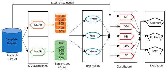
Figure 1.
The framework of the three groups of experiments A, B, and C.
5.3. Experimental Results
This part comprises three subsections. The first subsection presents the results of the Group A experiments where the baseline performance of the five classifiers is reported. The two other subsections depict the results of experimental Groups B and C in twelve column charts, six in each section, to show the performance of the five classifiers against the datasets when using two different imputation techniques, KNN and the mean (mode), with different ratios of missing values.
5.3.1. Baseline Performance
Table 2 shows the performance of each of the five classifiers on the six datasets without any missing values to report the baseline performance using accuracy, F1-score, and MCC metrics. The following are some observations from the baseline evaluation in Table 2:

Table 2.
The baseline performance of the classifiers evaluated by three measures.
- As stated in the literature [48,67,68], MCC is a more informative measure for classifier performance on imbalanced datasets, and therefore it provides a less truthful performance than both the accuracy and the F1-score, which report over-optimistic and inflated results.
- Though the impact of the imbalanced data on the performance of all classifiers is clear, it decreases dramatically on small, mixed, and imbalanced data, such as that of the Bank dataset.
- The performance of the naïve Bayes classifier decreased dramatically for the categorical imbalanced datasets because Gaussian naïve Bayes treats categorical data as if they are normally distributed; however, the data are made of up 0 s and 1 s, which makes it a non-sensible model with categorical datasets. In comparison with the other datasets, NB reported low performance ranging from 12% to 26% within the car and nursery datasets under different evaluation metrics. So, NB was excluded from experiments when dealing with categorical datasets.
5.3.2. Missing Values with MCAR Pattern
MCAR—Imputed with KNN
Figure 2a–c show the sensitivity of the five classifiers when using the KNN imputation technique on the six datasets with different ratios of NAs (10–50%). Generally speaking, and apart from the size of the datasets, the performance of the five classifiers degrades as the NA ratio increases. It was observed that the percentage of this degradation differs from one dataset to another according to two factors: the size of the dataset and the type of the dataset. The size of the dataset is not a factor with mixed datasets, but it can be taken into consideration when dealing with numeric datasets; for example, the degradation in the performance of all classifiers in the Iris dataset is higher than the degradation in the Dry Beans dataset due to the size factor. The size of the dataset is also a factor within categorical datasets; as shown in Figure 2a, the degradation of the classifiers in the Car dataset is higher than the degradation in the Nursery dataset. In terms of the dataset type, it can be said that all classifiers are highly sensitive to the NAs in categorical datasets. This is clear in Figure 2a. The NB classifier was excluded from the categorical datasets experiments because it is not a sensible model for categorical data. However, this cannot be noted in the numeric and mixed datasets as they do not give a clear performance for the classifiers. When using different evaluation metrics, i.e., MCC, F1-score, or accuracy, it was noted that the variation in the degradation ratios of all classifiers was smaller within numeric datasets. Within the Dry Beans dataset, DT, SVM, NB, LDA, and RF degraded by 3.63%, 2.80%, 2.18%, 3.46%, 2.53%, respectively, when evaluated by MCC; by 3%, 2.30%, 1.77%, 2.88%, 2.08%, and 3.15% when evaluated by F1-score; and by 2.35%, 1.87%, 3.19%, 2.14% when evaluated by accuracy. However, for categorical datasets, the degradation ratios in the performance of all classifiers were much higher when measured using the MCC than those reflected in either F1-score or accuracy for the same datasets. This means that MCC provides a more informative evaluation of the classifiers’ sensitivity to missing values. This is obviously clear with the SVM, which was degraded by an average of 71% when measured by MCC, whereas it was degraded by an average of 35% and 42% when measured by the F1-score and the accuracy, respectively, as shown in Figure 2a–c. Furthermore, within mixed datasets, the variation in the degradation ratios of all classifiers evaluated by MCC was clearly much higher than that of degradation ratios measured by the accuracy metric. This variation can be seen within all classifiers, especially DT and RF (Figure 2a,b), which degraded by around 43% when measured by MCC and by 8% when using the accuracy metric. This variation is due to an imbalanced dataset issue. Furthermore, SVM degradation shown in Figure 2a for the Bank dataset was much higher than its degradation shown in Figure 2c. The variation in the degradation ratios between MCC and F1-score cannot be reported within large mixed datasets, as they both give closer results. However, MCC reported higher degradation ratios within small mixed datasets (the Bank dataset).
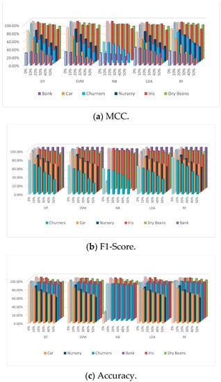
Figure 2.
Performance of the five classifiers on the six datasets with different ratios of MCAR MVs imputed using KNN.
MCAR Imputed with Mean (and Mode)
The numeric datasets were imputed using only the mean imputation technique, whereas the mixed datasets were imputed using both the mean and the mode imputation techniques. The classifiers behaved differently from one dataset to another as the NA ratio increased, as shown in Figure 3a–c. As in the KNN imputation technique, the two main factors to consider when evaluating the classifiers’ sensitivity to NAs are the size and the type of the datasets. Regarding the size factor considered with the numeric datasets, where the sensitivity of the classifiers to missing values decreased as the size of the dataset increased, the sensitivity of DT, SVM, NB, LDA, and RF within Iris and Dry Beans datasets evaluated by MCC was around 20%, 15%, 18%, 18%, and 15%, and 8%, 7%, 6%, 1%, and 6%, respectively. The size had no effect with mixed datasets; for example, the sensitivity of all classifiers within the bank dataset was around 1% or less, whereas the sensitivity of DT, SVM, NB, LDA, and RF within the Churners dataset evaluated by F1-score was around 36%, 38%, 21%, 28%, and 31%, respectively. In terms of the dataset type factor, there were no observations to be noted, however, the sensitivity of the classifiers can be reported for each dataset separately, e.g., for the Bank dataset, the classifiers were moderately sensitive to NAs when measured by MCC. DT, SVM, NB, LDA, and RF degraded by around 0.31%, 10.55%, 4.29%, 7.89%, and 8.92%, respectively. However, the classifiers were robust to the existence of NAs in the same dataset when measured by F1-acore and accuracy. DT, SVM, NB, LDA, and RF degraded by around 0.36%, 0.35%, 0.07%, 0.23%, and 0.19%, and 0.75%, 0.64%, 0.09%, 0.51%, and 0.38%, respectively. On the other hand, in the Churners dataset, all classifiers showed high sensitivity to the NAs when measured by either MCC or F1-score, whereas they showed less sensitivity when measured by the accuracy metric (Figure 3a–c). Evaluating the performance using different evaluation metrics, we made the same observation as in the first group of experiments when using the KNN imputation technique. The variation in the degradation ratios of all classifiers using the MCC metric was moderately higher than that of the F1-score and accuracy metrics within the numeric datasets (Figure 3a–c). In the mixed datasets, the degradation ratios evaluated by MCC were much higher than the degradation ratios evaluated by accuracy (Figure 3a–c). This is because of the imbalanced datasets issue, and was obvious with all classifiers. DT, SVM, NB, LDA, and RF were degraded by 35%,31%, 28%, 26%, and 30%, respectively, when measured using MCC, and were degraded by 7%, 5%, 5%, 4%, and 6%, respectively, when evaluated by the accuracy metric. The results of MCC and F1-score metrics within large mixed datasets could not be noted generally; however, the variation in the performance between them could be noted and reported within small mixed datasets.
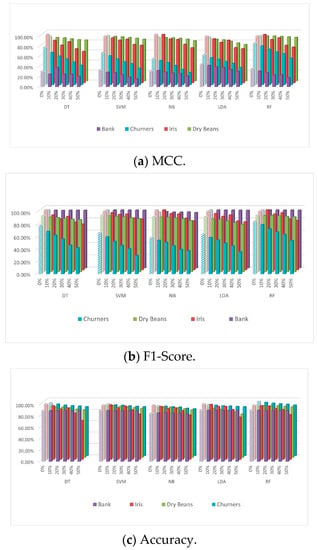
Figure 3.
Performance of the five classifiers on the six datasets with different ratios of MCAR MVs imputed using mean/mode.
5.3.3. Missing Values with MNAR Pattern
MNAR—Imputed with KNN
Figure 4a–c represent the performance of the five classifiers when using the KNN imputation technique to handle the missing values synthesized using the MNAR pattern, with different ratios of NAs (10–50%), in the six datasets. Generally, the classifiers’ performance was affected differently from one dataset to another as the NA ratio increased. The sensitivity of the five classifiers to the missing values was evaluated with regard to the size and type of the datasets. The size factor was reflected in only two cases. The first case was with the numeric datasets, where the sensitivity of the classifiers clearly decreased as the size of the dataset increased; for example, the sensitivity of DT, SVM, NB, LDA, and RF within the Iris and Dry Beans datasets evaluated by accuracy was around 31%, 29%, 29%, 35%, and 24%, respectively, and 12%, 11%, 23%, 22%, and 8%, respectively. The second case was with the mixed datasets under certain conditions, i.e., missing data should be synthesized using the MNAR pattern and imputed by the KNN imputation technique to be evaluated by MCC (Figure 4a). In terms of the type of dataset, the classifiers were highly to moderately sensitive with categorical datasets with different ratios. All classifiers were degraded by around 28% to 70% when the NA ratio increases from 10% to 50%. DT, SVM, LDA, and RF were degraded by around 30%, 65%, and 70% when evaluated by MCC, F1-score, and accuracy, respectively. In contrast, the sensitivity of the classifiers ranged from low to high with numeric datasets. The degradation ratio of classifiers ranged from around 10% to 50% (Figure 4). When the NA ratio increased, RF degraded by around 8% and 25%, depending on the size of the dataset. Furthermore, SVM degraded by 11% and 30%. For mixed datasets, the sensitivity of the classifiers differed based on the evaluation metric used, as each metric reports different sensitivity ratios. When using different evaluation metrics, it was clearly noted that the degradation ratios of all classifiers evaluated by the MCC metric were much higher than the degradation ratios evaluated by F1-score or accuracy metrics. This is because MCC considers the imbalanced datasets issue when evaluating the sensitivity. This could be clearly seen within mixed and numeric datasets, where the degradation ratios of all classifiers within the Iris dataset measured by MCC were much higher than the degradation ratios evaluated by F1-score or accuracy. The variation in the degradation ratios for all classifiers was closer in categorical datasets when evaluated by F1-score or accuracy metrics (Figure 4b,c). In the case of mixed datasets, the classifiers had lower sensitivity to NAs when evaluated by the accuracy metric (Figure 4c), whereas high sensitivity was reported for all classifiers in the mixed datasets when evaluated by MCC (Figure 4a). The sensitivity of the classifiers evaluated by F1-score is reported for each dataset separately (Figure 4b). Whereas all classifiers were robust against the existence of NAs in the Bank dataset, DT, SVM, and RF degraded by less than 1%, and LDA and NB degraded by around 3%. By comparison, the Churner dataset reported moderate to high sensitivity with all classifiers. DT, SVM, NB, LDA, and RF reported degradation ratios of 22%, 15%, 6%, 10%, and 27%, respectively.
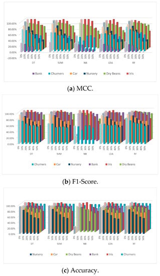
Figure 4.
Performance of the five classifiers on the six datasets with different ratios of MNAR MVs imputed using KNN.
MNAR—Imputed with Mean (and Mode)
The mean (mode) imputation technique was used for the four datasets, mixed and numeric, to handle missing data synthesized by the MNAR pattern through different NA ratios (10–50%); Figure 5a–c. All classifiers behaved differently from one dataset to another as the NA ratio increased. The two main factors to consider when evaluating the classifiers’ sensitivity to NAs are the size and the type of the datasets. The size factor was only reflected in two cases: first, the numeric datasets, where the sensitivity of the classifiers decreased as the size of the dataset increased. The size was not a factor with mixed datasets; however, it was reflected with mixed datasets within specific circumstances, which was the second case. NAs should be synthesized by the MNAR pattern to be imputed with the mean (mode) imputation technique and evaluated by MCC (Figure 5a). In terms of the dataset type, the sensitivity of the classifiers to the NAs with numeric datasets ranged from low to high sensitivity. Some classifiers drastically degraded as the NA ratio increased. SVM, NB, and LDA degraded by around 69%, 93%, and 97% respectively (Figure 5a). The sensitivity of the classifiers within mixed datasets ranged from low to moderate sensitivity, mainly when evaluated by F1-score or accuracy metrics (Figure 5b,c). When using the three evaluation measures, MCC, F1-score, and accuracy, and as reported in each of the above experiments, the degradation ratios of all classifiers evaluated by MCC were much higher than the ratios evaluated by either F1-score or accuracy metrics (Figure 5b,c). The sensitivity of the classifiers within large-size numeric datasets evaluated by MCC is somewhat close to their sensitivity when evaluated by either F1-score or accuracy metrics, whereas the small-size numeric dataset reported higher sensitivity using MCC compared to using F1-score or accuracy. Within mixed datasets, the sensitivity of the classifiers was robust or has low sensitivity when evaluated by the accuracy metric (Figure 5c). DT, SVM, NB, LDA, and RF degraded by around 2%, 2%, 1%, 3%, and 3%, respectively. Whereas the F1-score metric reported different sensitivity values with each of the mixed datasets (Figure 5b), the sensitivity of the classifiers with the Bank dataset did not exceed 2%. By comparison, with the Churner dataset, DT, SVM, NB, LDA, and RF degraded by 11%, 12%, 4%, 12%, and 16%, respectively. The MCC metric reported moderate to high sensitivity with mixed datasets ranging from 6% to 38% (Figure 5a). Table 3 summarizes the findings of the previous two sections (Section 5.3.2 and Section 5.3.3).
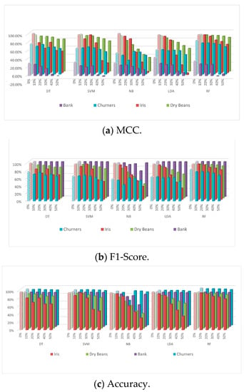
Figure 5.
Performance of the five classifiers on the six datasets with different ratios of MNAR MVs imputed using mean/mode.

Table 3.
Summary of the five classifiers’ performance with respect to the properties of the datasets and the two imputation techniques.
5.4. Discussion of the Results
This section summarizes and frames our findings of the depicted results of all experiments. To evaluate the overall effect of the MVs on the performance of the classifiers with regards to the MMs, IMs, size, and the type of the datasets, two groups of heat maps were generated to reflect the difference in the average performance of each classifier from its baseline. This difference was calculated using Equation (4).
where S is the sensitivity of a classifier, B is the baseline performance of the classifier, n is the number of ratios of MVs, i is the missing ratio, and a is the performance measure. Figure 6 and Figure 7 represent this sensitivity in two sets of heat maps for the MCAR and MNAR, respectively, using small (s) and large (L) datasets. From the two groups of figures, the following findings can be deduced:
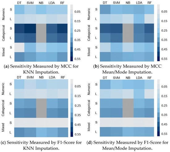
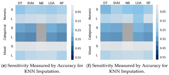
Figure 6.
Classifier sensitivity of the five classifiers on different sizes and types of dataset with MCAR MVs.
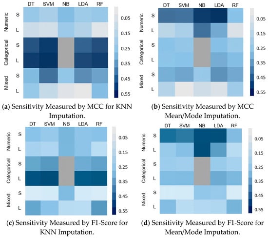
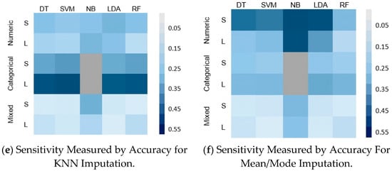
Figure 7.
Classifier sensitivity of the five classifiers on different sizes and types of dataset with MNAR MVs.
- In all cases, the performance of all classifiers was affected by the MVs for all datasets. The sensitivity of all classifiers to MVs was better reflected by the MCC than the accuracy and F1-score. This is obvious for the small datasets with mixed features; the accuracy and F1-score both show that there is no variation in the sensitivity of all classifiers, as shown in Figure 6c,d for the F1-Score and Figure 6e,f for the accuracy. However, the MCC shows that the SVM is the most affected, followed by the RF and then the LDA (Figure 6a,b).
- For the effect of the MMs, there was a noticeable difference between the sensitivity of the classifiers with each mechanism; these were more sensitive in the case of MNAR (Figure 7) than in the case of MCAR (Figure 6). This can be clearly observed in the case of large numeric and small mixed datasets.
- For the effect of the IMs, the pattern of the sensitivity is very similar in the case of MCAR. However, the classifiers show higher sensitivity with the KNN imputation (Figure 6a,c,e) than with the mean/mode imputation in Figure 6b,d,f. This implies that for a dataset with MVs due to MCAR, it would be advisable to use the mean/mode IM to ensure a performance that is almost near to the baseline. In the case of MNAR, the two IMs show different sensitivities, which imply the total dependency on the size and the type of the dataset.
- For the type of dataset, all classifiers show high sensitivity with categorical datasets; DT, SVM, LDA, and RF degraded by around 49%, 55%, 42%, and 52%, and 18%, 21%, 16%, and 20%, within the Car dataset when imputed by KNN and evaluated by MCC and F1-score, respectively. The sensitivity ranged from moderate to low with numeric and mixed datasets depending on the evaluation metric; DT, SVM, NB, LDA, and RF degraded by around 0.31%, 10.55%, 4.29%, 7.89%, and 8.92%, respectively, within the Bank dataset when evaluated by MCC, except for the case when MNAR data was imputed with the mean/mode, when numeric datasets showed the highest effect, as shown in Figure 7b,d,f.
- In the MCAR, DT among the five tested classifiers was the most sensitive to the MVs for all datasets, except the categorical data where the SVM was more sensitive as it showed more degradation in its performance from the baseline. The less sensitive classifiers were NB, LDA, and RF (Figure 6).
- In the MNAR, NB and LDA were the two most sensitive classifies, especially in the case of using the mean/mode IMs (Figure 7b,d,f).
6. Conclusions
It is widely known that improving and maintaining data quality is an important challenge, especially for ensuring the output quality of data analytics platforms. Thus, this paper investigates the influence of having incomplete data, with different ratios of MVs and different patterns (MCAR and MNAR), on five classifiers tested against six different datasets through 630 experiments. To better judge the accuracy of the results, three evaluation metrics, MCC, accuracy, and F1-score, were applied. The results can be summarized into five main findings. First, the sensitivity of the classifiers increases as the percentage of MVs increases. Second, the sensitivity of the classifiers to MVs that result from the MCAR pattern is lower than its sensitivity compared with the MNAR pattern. Third, the best imputation method in most cases is the mean (and mode) when there are MVs with the MCAR pattern; however, this is dependent on the size and type of dataset when there are MVs with the MNAR pattern. Fourth, in all the experiments conducted during this study, the MCC evaluation metric was the best measure as it gave more reliable and informative results. This is because MCC considers the imbalanced dataset factor when evaluating the classifiers. On the other hand, F1-score and accuracy metrics gave misleading results that did not reflect reality. Fifth, the most sensitive classifiers in the case of MCAR are DT and SVM, whereas NB, LDA, and RF are less sensitive. In contrast, in the case of MNAR, NB and LDA are more sensitive to NAs. Although the machine learning models proved our theory that the existence of NAs somehow affects the models’ performance, we will use deep learning models such as convolutional neural networks (CNNs) in our future works to obtain a clearer picture of the effect of missing values on different learning models.
Author Contributions
M.I.G.: Conceptualization, Data Curation, Resources, Software, Visualization, Writing—original draft preparation. Y.M.H.: Supervision, Writing—review and editing. D.S.E.: Conceptualization, Methodology, Validation, Supervision, Visualization, Writing—review and editing. All authors have read and agreed to the published version of the manuscript.
Funding
This research received no external funding.
Data Availability Statement
The six datasets that have been used in this study are downloaded from the UCI (https://archive.ics.uci.edu/ml/datasets.php) and Kagle (https://www.kaggle.com/datasets) repositories.
Conflicts of Interest
The authors declare no conflict of interest.
References
- Gabr, M.I.; Mostafa, Y.; Elzanfaly, D.S. Data Quality Dimensions, Metrics, and Improvement Techniques. Future Comput. Inform. J. 2021, 6, 3. [Google Scholar] [CrossRef]
- Pedersen, A.B.; Mikkelsen, E.M.; Cronin-Fenton, D.; Kristensen, N.R.; Pham, T.M.; Pedersen, L.; Petersen, I. Missing data and multiple imputation in clinical epidemiological research. Clin. Epidemiol. 2017, 9, 157. [Google Scholar] [CrossRef] [PubMed]
- Aleryani, A.; Wang, W.; De La Iglesia, B. Multiple imputation ensembles (MIE) for dealing with missing data. SN Comput. Sci. 2020, 1, 134. [Google Scholar] [CrossRef]
- Blomberg, L.C.; Ruiz, D.D.A. Evaluating the influence of missing data on classification algorithms in data mining applications. In Proceedings of the Anais do IX Simpósio Brasileiro de Sistemas de Informação, SBC, Porto Alegre, Brazil, 22 May 2013; pp. 734–743. [Google Scholar]
- Acuna, E.; Rodriguez, C. The treatment of missing values and its effect on classifier accuracy. In Classification, Clustering, and Data Mining Applications; Springer: Berlin/Heidelberg, Germany, 2004; pp. 639–647. [Google Scholar]
- Jäger, S.; Allhorn, A.; Bießmann, F. A benchmark for data imputation methods. Front. Big Data 2021, 4, 693674. [Google Scholar] [CrossRef] [PubMed]
- Gimpy, M. Missing value imputation in multi attribute data set. Int. J. Comput. Sci. Inf. Technol. 2014, 5315, 5321. [Google Scholar]
- You, J.; Ma, X.; Ding, Y.; Kochenderfer, M.J.; Leskovec, J. Handling missing data with graph representation learning. Adv. Neural Inf. Process. Syst. 2020, 33, 19075–19087. [Google Scholar]
- Samant, R.; Rao, S. Effects of missing data imputation on classifier accuracy. Int. J. Eng. Res. Technol. IJERT 2013, 2, 264–266. [Google Scholar]
- Christopher, S.Z.; Siswantining, T.; Sarwinda, D.; Bustaman, A. Missing value analysis of numerical data using fractional hot deck imputation. In Proceedings of the 2019 3rd International Conference on Informatics and Computational Sciences (ICICoS), Semarang, Indonesia, 29–30 October 2019; pp. 1–6. [Google Scholar]
- Aljuaid, T.; Sasi, S. Proper imputation techniques for missing values in data sets. In Proceedings of the 2016 International Conference on Data Science and Engineering (ICDSE), Cochin, India, 23–25 August 2016; pp. 1–5. [Google Scholar]
- Thirukumaran, S.; Sumathi, A. Missing value imputation techniques depth survey and an imputation algorithm to improve the efficiency of imputation. In Proceedings of the 2012 Fourth International Conference on Advanced Computing (ICoAC), Chennai, India, 13–15 December 2012; pp. 1–5. [Google Scholar]
- Hossin, M.; Sulaiman, M.; Mustapha, A.; Mustapha, N.; Rahmat, R. A hybrid evaluation metric for optimizing classifier. In Proceedings of the 2011 3rd Conference on Data Mining and Optimization (DMO), Kuala Lumpur, Malaysia, 28–29 June 2011; pp. 165–170. [Google Scholar]
- Bekkar, M.; Djemaa, H.K.; Alitouche, T.A. Evaluation measures for models assessment over imbalanced data sets. J. Inf. Eng. Appl. 2013, 3, 27–29. [Google Scholar]
- Tharwat, A. Classification assessment methods. Appl. Comput. Inform. 2021, 17, 168–192. [Google Scholar] [CrossRef]
- Chicco, D.; Warrens, M.J.; Jurman, G. The Matthews correlation coefficient (MCC) is more informative than Cohen’s Kappa and Brier score in binary classification assessment. IEEE Access 2021, 9, 78368–78381. [Google Scholar] [CrossRef]
- Chicco, D.; Tötsch, N.; Jurman, G. The Matthews correlation coefficient (MCC) is more reliable than balanced accuracy, bookmaker informedness, and markedness in two-class confusion matrix evaluation. BioData Min. 2021, 14, 13. [Google Scholar] [CrossRef]
- Warrens, M.J. Five ways to look at Cohen’s kappa. J. Psychol. Psychother. 2015, 5, 1000197. [Google Scholar] [CrossRef]
- Jeni, L.A.; Cohn, J.F.; De La Torre, F. Facing imbalanced data–recommendations for the use of performance metrics. In Proceedings of the 2013 Humaine Association Conference on Affective Computing and Intelligent Interaction, Geneva, Switzerland, 2–5 September 2013; pp. 245–251. [Google Scholar]
- Narkhede, S. Understanding auc-roc curve. Towards Data Sci. 2018, 26, 220–227. [Google Scholar]
- Nanmaran, R.; Srimathi, S.; Yamuna, G.; Thanigaivel, S.; Vickram, A.; Priya, A.; Karthick, A.; Karpagam, J.; Mohanavel, V.; Muhibbullah, M. Investigating the role of image fusion in brain tumor classification models based on machine learning algorithm for personalized medicine. Comput. Math. Methods Med. 2022, 2022, 7137524. [Google Scholar] [CrossRef]
- Sokolova, M.; Lapalme, G. A systematic analysis of performance measures for classification tasks. Inf. Process. Manag. 2009, 45, 427–437. [Google Scholar] [CrossRef]
- Jadhav, A.S. A novel weighted TPR-TNR measure to assess performance of the classifiers. Expert Syst. Appl. 2020, 152, 113391. [Google Scholar] [CrossRef]
- Liu, P.; Lei, L.; Wu, N. A quantitative study of the effect of missing data in classifiers. In Proceedings of the the Fifth International Conference on Computer and Information Technology (CIT’05), Shanghai, China, 21–23 September 2005; pp. 28–33. [Google Scholar]
- Hunt, L.A. Missing data imputation and its effect on the accuracy of classification. In Data Science; Springer: Berlin/Heidelberg, Germany, 2017; pp. 3–14. [Google Scholar]
- Purwar, A.; Singh, S.K. Hybrid prediction model with missing value imputation for medical data. Expert Syst. Appl. 2015, 42, 5621–5631. [Google Scholar] [CrossRef]
- Su, X.; Khoshgoftaar, T.M.; Greiner, R. Using imputation techniques to help learn accurate classifiers. In Proceedings of the 2008 20th IEEE International Conference on Tools with Artificial Intelligence, Dayton, OH, USA, 3–5 November 2008; Volume 1, pp. 437–444. [Google Scholar]
- Jordanov, I.; Petrov, N.; Petrozziello, A. Classifiers accuracy improvement based on missing data imputation. J. Artif. Intell. Soft Comput. Res. 2018, 8, 31–48. [Google Scholar] [CrossRef]
- Luengo, J.; García, S.; Herrera, F. On the choice of the best imputation methods for missing values considering three groups of classification methods. Knowl. Inf. Syst. 2012, 32, 77–108. [Google Scholar] [CrossRef]
- Garciarena, U.; Santana, R. An extensive analysis of the interaction between missing data types, imputation methods, and supervised classifiers. Expert Syst. Appl. 2017, 89, 52–65. [Google Scholar] [CrossRef]
- Aggarwal, U.; Popescu, A.; Hudelot, C. Active learning for imbalanced datasets. In Proceedings of the IEEE/CVF Winter Conference on Applications of Computer Vision (WACV), Snowmass village, Snowmass Village, CO, USA, 1–7 October 2020; pp. 1428–1437. [Google Scholar]
- García, V.; Mollineda, R.A.; Sánchez, J.S. Theoretical analysis of a performance measure for imbalanced data. In Proceedings of the 2010 20th International Conference on Pattern Recognition, Washington, DC, USA, 23–26 August 2010; pp. 617–620. [Google Scholar]
- Lei, L.; Wu, N.; Liu, P. Applying sensitivity analysis to missing data in classifiers. In Proceedings of the ICSSSM’05, 2005 International Conference on Services Systems and Services Management, Chongqing, China, 13–15 June 2005; Volume 2, pp. 1051–1056. [Google Scholar]
- de la Vega de León, A.; Chen, B.; Gillet, V.J. Effect of missing data on multitask prediction methods. J. Cheminform. 2018, 10, 26. [Google Scholar] [CrossRef] [PubMed]
- Hossain, T.; Inoue, S. A comparative study on missing data handling using machine learning for human activity recognition. In Proceedings of the 2019 Joint 8th International Conference on Informatics, Electronics & Vision (ICIEV) and 2019 3rd International Conference on Imaging, Vision & Pattern Recognition (icIVPR), Spokane, WA, USA, 30 May–2 June 2019; pp. 124–129. [Google Scholar]
- Wang, G.; Lu, J.; Choi, K.S.; Zhang, G. A transfer-based additive LS-SVM classifier for handling missing data. IEEE Trans. Cybern. 2018, 50, 739–752. [Google Scholar] [CrossRef] [PubMed]
- Makaba, T.; Dogo, E. A comparison of strategies for missing values in data on machine learning classification algorithms. In Proceedings of the 2019 International Multidisciplinary Information Technology and Engineering Conference (IMITEC), Vanderbijlpark, South Africa, 21–22 November 2019; pp. 1–7. [Google Scholar]
- Liu, Q.; Hauswirth, M. A provenance meta learning framework for missing data handling methods selection. In Proceedings of the 11th IEEE Annual Ubiquitous Computing, Electronics & Mobile Communication Conference (UEMCON), Virtual Conference, 28–31 October 2020; pp. 0349–0358. [Google Scholar]
- Izonin, I.; Tkachenko, R.; Verhun, V.; Zub, K. An approach towards missing data management using improved GRNN-SGTM ensemble method. Eng. Sci. Technol. Int. J. 2021, 24, 749–759. [Google Scholar] [CrossRef]
- Han, J.; Kamber, M.; Pei, J. Data mining: Concepts and techniques. Morgan Kaufinann 2006, 10, 88–89. [Google Scholar]
- Malarvizhi, M.; Thanamani, A. K-NN classifier performs better than K-means clustering in missing value imputation. IOSR J. Comput. Eng. 2012, 6, 12–15. [Google Scholar] [CrossRef]
- Singhai, R. Comparative analysis of different imputation methods to treat missing values in data mining environment. Int. J. Comput. Appl. 2013, 82, 34–42. [Google Scholar] [CrossRef]
- Golino, H.F.; Gomes, C.M. Random forest as an imputation method for education and psychology research: Its impact on item fit and difficulty of the Rasch model. Int. J. Res. Method Educ. 2016, 39, 401–421. [Google Scholar] [CrossRef]
- Nishanth, K.J.; Ravi, V. Probabilistic neural network based categorical data imputation. Neuro Comput. 2016, 218, 17–25. [Google Scholar] [CrossRef]
- Grandini, M.; Bagli, E.; Visani, G. Metrics for multi-class classification: An overview. arXiv 2020, arXiv:2008.05756. [Google Scholar]
- Luque, A.; Carrasco, A.; Martín, A.; de Las Heras, A. The impact of class imbalance in classification performance metrics based on the binary confusion matrix. Pattern Recognit. 2019, 91, 216–231. [Google Scholar] [CrossRef]
- Branco, P.; Torgo, L.; Ribeiro, R.P. A survey of predictive modeling on imbalanced domains. ACM Comput. Surv. CSUR 2016, 49, 1–50. [Google Scholar] [CrossRef]
- Chicco, D.; Jurman, G. The advantages of the Matthews correlation coefficient (MCC) over F1 score and accuracy in binary classification evaluation. BMC Genom. 2020, 21, 6. [Google Scholar] [CrossRef]
- Sa’id, A.A.; Rustam, Z.; Wibowo, V.V.P.; Setiawan, Q.S.; Laeli, A.R. Linear support vector machine and logistic regression for cerebral infarction classification. In Proceedings of the 2020 International Conference on Decision Aid Sciences and Application (DASA), Online, 8–9 November 2020; pp. 827–831. [Google Scholar]
- Cao, C.; Chicco, D.; Hoffman, M.M. The MCC-F1 curve: A performance evaluation technique for binary classification. arXiv 2020, arXiv:2006.11278. [Google Scholar]
- AlBeladi, A.A.; Muqaibel, A.H. Evaluating compressive sensing algorithms in through-the-wall radar via F1-score. Int. J. Signal Imaging Syst. Eng. 2018, 11, 164–171. [Google Scholar] [CrossRef]
- Glazkova, A. A comparison of synthetic oversampling methods for multi-class text classification. arXiv 2020, arXiv:2008.04636. [Google Scholar]
- Toupas, P.; Chamou, D.; Giannoutakis, K.M.; Drosou, A.; Tzovaras, D. An intrusion detection system for multi-class classification based on deep neural networks. In Proceedings of the 2019 18th IEEE International Conference on Machine Learning And Applications (ICMLA), Boca Raton, FL, USA, 16–19 December 2019; pp. 1253–1258. [Google Scholar]
- Wang, R.; Fan, J.; Li, Y. Deep multi-scale fusion neural network for multi-class arrhythmia detection. IEEE J. Biomed. Health Inform. 2020, 24, 2461–2472. [Google Scholar] [CrossRef]
- Bouazizi, M.; Ohtsuki, T. Multi-class sentiment analysis in Twitter: What if classification is not the answer. IEEE Access 2018, 6, 64486–64502. [Google Scholar] [CrossRef]
- Baker, C.; Deng, L.; Chakraborty, S.; Dehlinger, J. Automatic multi-class non-functional software requirements classification using neural networks. In Proceedings of the 2019 IEEE 43rd Annual Computer Software and Applications Conference (COMPSAC), Milwaukee, WI, USA, 15–19 July 2019; Volume 2, pp. 610–615. [Google Scholar]
- Liu, C.; Osama, M.; De Andrade, A. DENS: A dataset for multi-class emotion analysis. arXiv 2019, arXiv:1910.11769. [Google Scholar]
- Opitz, J.; Burst, S. Macro f1 and macro f1. arXiv 2019, arXiv:1911.03347. [Google Scholar]
- Josephine, S.A. Predictive Accuracy: A Misleading Performance Measure for Highly Imbalanced Data Classified negative. In Proceedings of the SAS Global Forum, Orlando, FL, USA, 2–5 April 2017. [Google Scholar]
- Boughorbel, S.; Jarray, F.; El-Anbari, M. Optimal classifier for imbalanced data using Matthews Correlation Coefficient metric. PLoS ONE 2017, 12, e0177678. [Google Scholar] [CrossRef]
- Fisher, R. UCI Iris Data Set. 1988. Available online: https://archive.ics.uci.edu/ml/datasets/iris (accessed on 18 April 2022).
- Moro, S.; Paulo, C.; Paulo, R. UCI Bank Marketing Data Set. 2014. Available online: https://archive.ics.uci.edu/ml/ (accessed on 21 April 2022).
- Bohanec, M.; Zupan, B. UCI Nursery Data Set. 1997. Available online: https://archive.ics.uci.edu/ml/datasets/nursery (accessed on 21 April 2022).
- Bohanec, M. Car Evaluation Data Set. 1997. Available online: https://www.kaggle.com/datasets/elikplim/car-evaluation-data-setl (accessed on 21 April 2022).
- Mehmet, A. Churn for Bank Customers. 2020. Available online: https://www.kaggle.com/datasets/mathchi/churn-for-bank-customers (accessed on 21 April 2022).
- Elawady, A.; Iskander, G. Dry Beans Classification. 2021. Available online: https://kaggle.com/competitions/dry-beans-classification-iti-ai-pro-intake01 (accessed on 21 April 2022).
- Gong, M. A novel performance measure for machine learning classification. Int. J. Manag. Inf. Technol. IJMIT 2021, 13, 1–19. [Google Scholar] [CrossRef]
- Chicco, D.; Jurman, G. An invitation to greater use of Matthews correlation coefficient (MCC) in robotics and artificial intelligence. Front. Robot. AI 2022, 9, 78. [Google Scholar] [CrossRef] [PubMed]
Disclaimer/Publisher’s Note: The statements, opinions and data contained in all publications are solely those of the individual author(s) and contributor(s) and not of MDPI and/or the editor(s). MDPI and/or the editor(s) disclaim responsibility for any injury to people or property resulting from any ideas, methods, instructions or products referred to in the content. |
© 2023 by the authors. Licensee MDPI, Basel, Switzerland. This article is an open access article distributed under the terms and conditions of the Creative Commons Attribution (CC BY) license (https://creativecommons.org/licenses/by/4.0/).