Article

Is My Pruned Model Trustworthy? PE-Score: A New CAM-Based Evaluation Metric

Doctorado en Ingeniería, Universidad Militar Nueva Granada, Bogota 110111, Colombia
*
Author to whom correspondence should be addressed.
These authors contributed equally to this work.
Big Data Cogn. Comput. 2023, 7(2), 111; https://doi.org/10.3390/bdcc7020111
Submission received: 11 May 2023 / Revised: 29 May 2023 / Accepted: 2 June 2023 / Published: 6 June 2023

Abstract

:
One of the strategies adopted to compress CNN models for image classification tasks is pruning, where some elements, channels or filters of the network are discarded. Typically, pruning methods present results in terms of model performance before and after pruning (assessed by accuracy or a related parameter such as the F1-score), assuming that if the difference is less than a certain value (e.g., 2%), the pruned model is trustworthy. However, state-of-the-art models are not concerned with measuring the actual impact of pruning on the network by evaluating the pixels used by the model to make the decision, or the confidence of the class itself. Consequently, this paper presents a new metric, called the Pruning Efficiency score (PE-score), which allows us to identify whether a pruned model preserves the behavior (i.e., the extracted patterns) of the unpruned model, through visualization and interpretation with CAM-based methods. With the proposed metric, it will be possible to better compare pruning methods for CNN-based image classification models, as well as to verify whether the pruned model is efficient by focusing on the same patterns (pixels) as those of the original model, even if it has reduced the number of parameters and FLOPs.

1. Introduction

One of the strategies for the compression of CNN-based models (convolutional neural networks) is pruning, where the goal is to reduce the size of the model while preserving its performance (e.g., accuracy) as much as possible [1,2,3]. There are many works in the literature related to pruning, such as weight-based methods with the L1-norm [4,5] or L2-norm [6,7], which assume that the filters or feature maps with the least impact on the network are those with the smallest size. Other methods use, for example, the Taylor expansion [8] or the gradients [9,10] to select the elements, channels or filters to be discarded in the process. However, regardless of the type of pruning criteria used, most state-of-the-art works consolidate their results by evaluating three factors: model performance, model size and computational cost. Accuracy (i.e., final accuracy, accuracy drop) and other similar metrics, such as the F1-score, are often used to evaluate the performance. The model size is measured as a function of the number of parameters, while the computational cost is determined by the number of FLOPs (floating point operations) [11,12,13,14]. In this way, the reduction results of the pruned model with respect to the unpruned model can be quantified, taking into account that the smaller the reduction in accuracy (or the smaller the increase in error) and the greater the reduction in both parameters and FLOPs, the better the pruned model.
In order to compare different pruned models and select the best one, it is necessary that the models are trained and validated on the same set of images, either specific or general purpose (benchmark dataset) [2]. A typical dataset for comparison is CIFAR10, which has 60,000 images of 10 classes, distributed across 50,000 images for training and 10,000 images for validation [15]. In this case, unpruned models of VGG16 with 134 million parameters and 31 G-FLOPs for CIFAR10 have been reported in the literature, reaching accuracy of 94.86% [16].
Since the goal of pruned methods is to maintain maximum accuracy with the greatest possible reduction in FLOPs and parameters, Table 1 shows a comparison of representative state-of-the-art pruning methods, in terms of the accuracy of the pruned model, FLOPs and parameter reduction. The difference between them in terms of accuracy is less than 1%, but in terms of FLOPs reduction and parameter reduction, it exceeds 25%.
Considering that other works have reported results in terms of the accuracy drop and FLOPs reduction, Table 2 shows a comparison of some of these pruning methods. As can be seen, the greater the reduction in FLOPs, the greater the expected decrease in the accuracy of the pruned model.
Beyond the pruning criteria used to select the elements, channels [10,18,20] or filters [12,16,21,22] to discard, the methods also differ in the pruning rate per layer. For example, the same percentage of pruned filters can be applied to all layers (Uniform Pruning Rate, UPR) [16], or this percentage can be varied in an ascending, descending or fluctuating manner (Adaptive Pruning Rate, APR) [19]. Considering that most of the parameters are in FC (fully connected) layers and most of the FLOPs are in convolutional layers [3], upward pruning will significantly reduce the number of parameters, with a small reduction in the number of FLOPs, while downward pruning will significantly reduce the number of FLOPs, with a small reduction in the number of parameters. Hence, when applying APR, the reduction percentages for both parameters and FLOPs will be different [4,8,9,13,17].
Therefore, if several pruned models of similar performance, obtained from different pruning criteria and rates per layer, are available, it is pertinent to ask how to choose the best among them. Similarly, how can we verify that the pruned model is efficient, i.e., that the pruned model can identify the same patterns with a smaller number of parameters and/or FLOPs? Pruned models are typically evaluated in terms of the difference in accuracy, FLOPs and parameters relative to the original model, but not in terms of their reliability, and, to the best of our knowledge, these questions have not been answered in the state of the art.
Accordingly, this paper focuses on the reliability analysis of pruned CNN models, with the following contributions.
  • A metric to evaluate the reliability of pruned models that is independent of both the criterion and the pruning rate is proposed (PE-score). This metric is calculated from two similarity measures ( S S I M and I o U ) and from the confidence variance of the class. The S S I M (Structural Similarity Index Measure) and I o U (Intersection over Union) are computed between the class activation maps of the original and pruned models, using a CAM (Class Activation Map) type method, such as Grad-CAM++ [23].
  • The importance of the PE-score is shown through a reliability analysis of the pruned models. Two different pruning methods (Weight and SeNPIS-Faster) are evaluated for two sets of images (CIFAR10 and COVID-19), concluding that a reliable pruned model is not only the one that preserves the accuracy of the original model, but also the one that performs image classification based on the same patterns (pixels) as the unpruned model.
  • A procedure for selecting the PR (pruning rate) value is also provided, to ensure that the pruned model is trustworthy.
The remainder of the work is organized as follows. Section 2 presents preliminary concepts regarding accuracy in image classification models, pruning and CAM-based methods for the visualization and interpretation of CNNs. Section 3 describes the materials and methods used to obtain the proposed metric, called the PE-score. Section 4 shows the results of the PE-score for two datasets, two pruning methods and six pruning rates. Section 5 discusses the results of the experimental phase. Finally, Section 6 concludes the study.

2. Background

2.1. Accuracy in Image Classification Models

Pruned models are usually evaluated in terms of three elements: performance, size and computational cost. Size is measured by the number of parameters, and computational cost by the number of FLOPs. On the other hand, performance can be evaluated in terms of accuracy (or a similar metric, such as the F1-score) or loss (such as cross-entropy). The difference between the original model and the pruned model is then calculated (e.g., accuracy drop [11]), and, usually, the model with the smallest drop in accuracy and the highest number of FLOPs and/or the lowest number of parameters is selected.
However, what is the downside of measuring the reliability of pruned models based solely on accuracy reduction? First, let us review the definition of accuracy according to Equation (1):
a c c = T P + T N T P + T N + F P + F N ,
where TP (True Positive) corresponds to the correctly classified positive class images, TN (True Negative) corresponds to the correctly classified negative class images, FP (False Positive) corresponds to the incorrectly classified negative images and FN (False Negative) corresponds to the incorrectly classified positive images.
Let us now assume an unpruned model whose evaluation gives T P = 850 , T N = 850 , F P = 150 , F N = 150 , i.e., a c c = 0.85 . Pruning the model using two different methods yields m o d e l 1 with T P = 800 , T N = 800 , F P = 200 , F N = 200 and m o d e l 2 with T P = 950 , T N = 650 , F P = 350 , F N = 50 . The accuracy of both pruned models is a c c = 0.8 , and the loss of accuracy compared to the unpruned model is 5 percentage points. Could we rely on the two pruned models based solely on the change in accuracy? It is clear that m o d e l 2 is biased (i.e., toward class “1”) and is not as reliable as m o d e l 1 , even though they have the same accuracy value. Some might say that the solution can be found in the F1-score metric, which drops sharply when the model is biased toward one class. However, what happens if the dataset contains distractors? Suppose that we have an original model that correctly identifies the representative patterns of the class, and we obtain a pruned model that classifies correctly but focuses on the distractors and not on the correct patterns. Could such a pruned model be trusted based only on metrics such as the accuracy or F1-score?
In addition to preserving the model’s classification rate, an important aspect is that the pruned model preserves the patterns on which it based its classification decision. In other words, if the original model, for example, focuses on the cat’s nose to identify that the image corresponds to a cat and not a dog, a reliable pruned model will be one that also focuses on the cat’s nose. Therefore, the analysis of reliable pruned models should be based on the comparison of the discriminative zones before and after pruning, using some method of visualizing and interpreting CNNs.

2.2. Pruning

Models based on CNNs have proven to be very useful in image classification tasks. However, many of them have a large number of parameters, which makes them “heavy” in edge computing solutions, while their inference times do not allow the processing of a large number of images per second [24]. Considering the variety of applications that can benefit from this type of model (e.g., Industry 4.0), it is crucial to apply efficient methods to reduce the complexity of the model (i.e., reduce parameters and FLOPs) without compromising its performance. In this context, among the model compression mechanisms, pruning has proven to be the most efficient to achieve the previously described purpose [25].
To illustrate the concept of pruning in CNNs, Figure 1 shows an example for NNs (neural networks) that can be easily extrapolated to CNNs. The original network (left) has three layers, as follows: an input layer with three neurons, a hidden layer with five neurons and an output layer with two neurons. Pruning does not affect the input layer or the output layer, so, for this example, it only affects the hidden layer. Let us assume that PR = 40%, which means that of the five neurons in the hidden layer, two neurons need to be pruned (i.e., removed from the network), leaving three neurons in the pruned network. Once the PR value is selected, the next step is to apply a pruning criterion, e.g., weight-based, such as the L1-norm or L2-norm. The pruned network (right) will then contain the neurons considered most important for the model, according to the pruning criterion selected.
In the case of CNNs, pruning can be applied to channels (of filters), filters and layers. However, the most common state-of-the-art pruning method is at the filter level, as applied in the present study.

2.3. Visualization Methods

One of the drawbacks of classification models based on DL (deep learning) is that they resemble a black box, since it is not intuitive which types of patterns the model has learned and whether they are the most appropriate ones to identify each of the classes. Thus, it is necessary to use a visualization method that allows us to identify the discriminative regions of the image, i.e., the pixels on which the model based its decision. One of the first visualization methods corresponds to CAM, which is a weakly supervised object localization method that can perform two tasks simultaneously in a single forward pass: first, classify the image, and second, detect specific regions of the class [26]. Its output is a heatmap highlighting the pixels used by the model to perform the categorization. Although the method is very easy to implement in CNNs, its disadvantage lies in the fact that it requires a modification of the network, since the FC layers must be eliminated and replaced by global average pooling before the classification layer.
A second group of methods for the visualization and interpretation of CNNs corresponds to Grad-CAM and Grad-CAM++, which rely on the gradients flowing in the last convolutional layer to identify pixels of interest in the image [23,27]. However, Grad-CAM++ has shown better pixel identification when there are multiple objects of the same class. Unlike CAM, both Grad-CAM and Grad-CAM++ do not require network modifications for their computation. In addition, there are other methods that do not rely on the gradient, such as Ablation-CAM, which uses ablation analysis to determine the class-discriminative importance of individual feature maps [28].
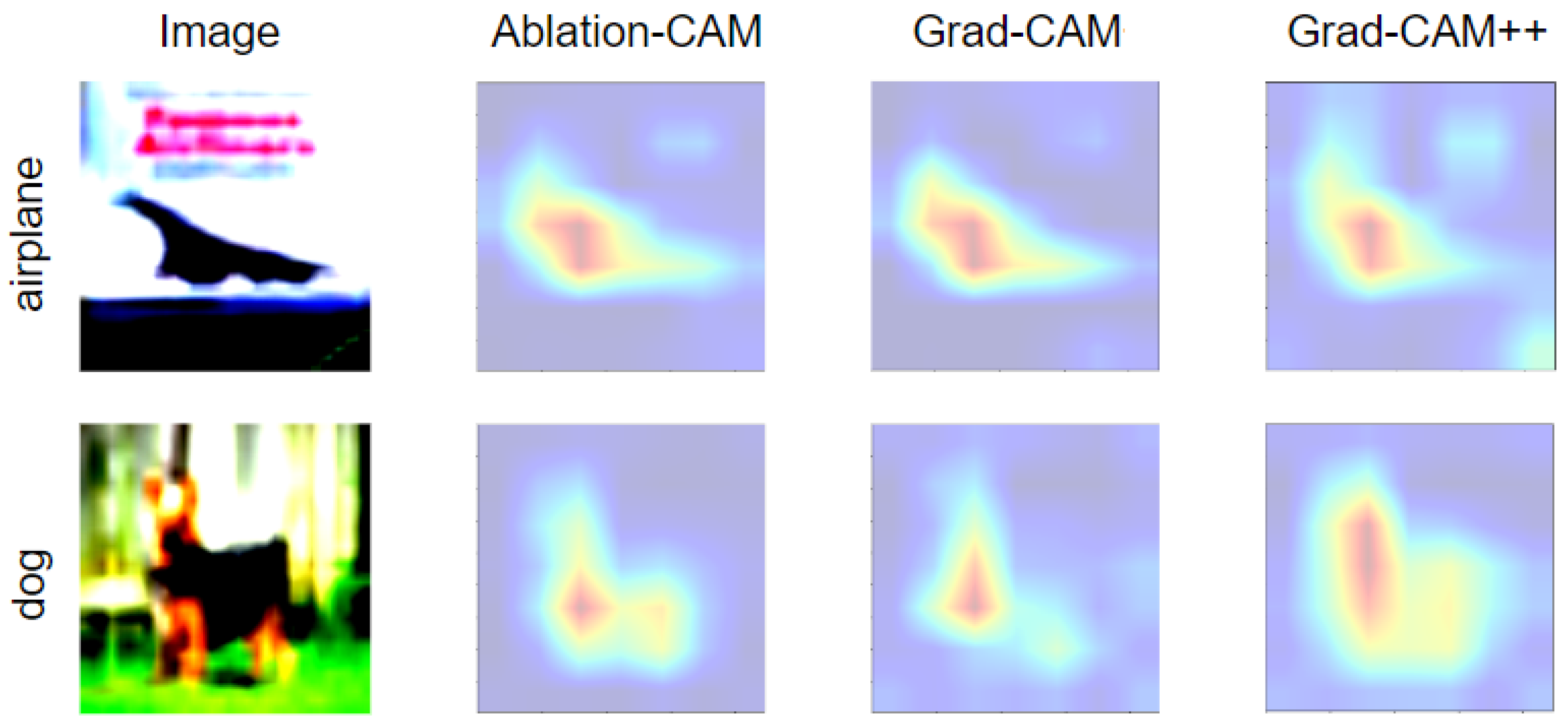
Figure 2 shows examples of visual explanation maps using CAM-based methods. Regardless of the visualization method used, the goal is to completely and concretely identify the image pixels recognized by the model to perform the classification.
As can be seen in the figure above, the pixels activated using the same network and input image vary between the different visualization methods. Of the three CAM-based selected methods for CIFAR10 images, the one that best identifies the pixels associated with the class corresponds to Grad-CAM++.

3. Materials and Methods

One of the advantages of deep learning over traditional ML (machine learning) is that, in DL, pattern extraction is performed directly by the model, while, in ML, it is performed manually [29]. In this way, the filters that extract patterns for decision making from the model are updated on each training iteration. Therefore, if a model has been trained with a set of images and identifies the representative patterns of each of the classes, the new model, when pruned, should have a similar behavior, i.e., focus on the same group of pixels as the original model. Otherwise, if the pruned model bases its decision on a different group of pixels of the image, it implies that the model is not reliable, even if the categorization is done correctly.
Taking into account the above, the PE-score is proposed, which is calculated from two similarity metrics and a confidence variance metric. The first two metrics are computed from the heatmaps of the original and pruned models: first, by a global similarity using S S I M , and second, by a specific similarity of the highlighted pixels using I o U . The last one is performed by calculating the difference between the class confidence of the original model and that of the pruned model. In all three cases, the values range from 0 to 1. For both S S I M and I o U , the best value is 1 and the worst is 0, while, for the confidence variation, the best value is 0 and the worst is 1. Therefore, the PE-score is within the range of 0 to 1, with the best value being 1 and the worst value being 0.
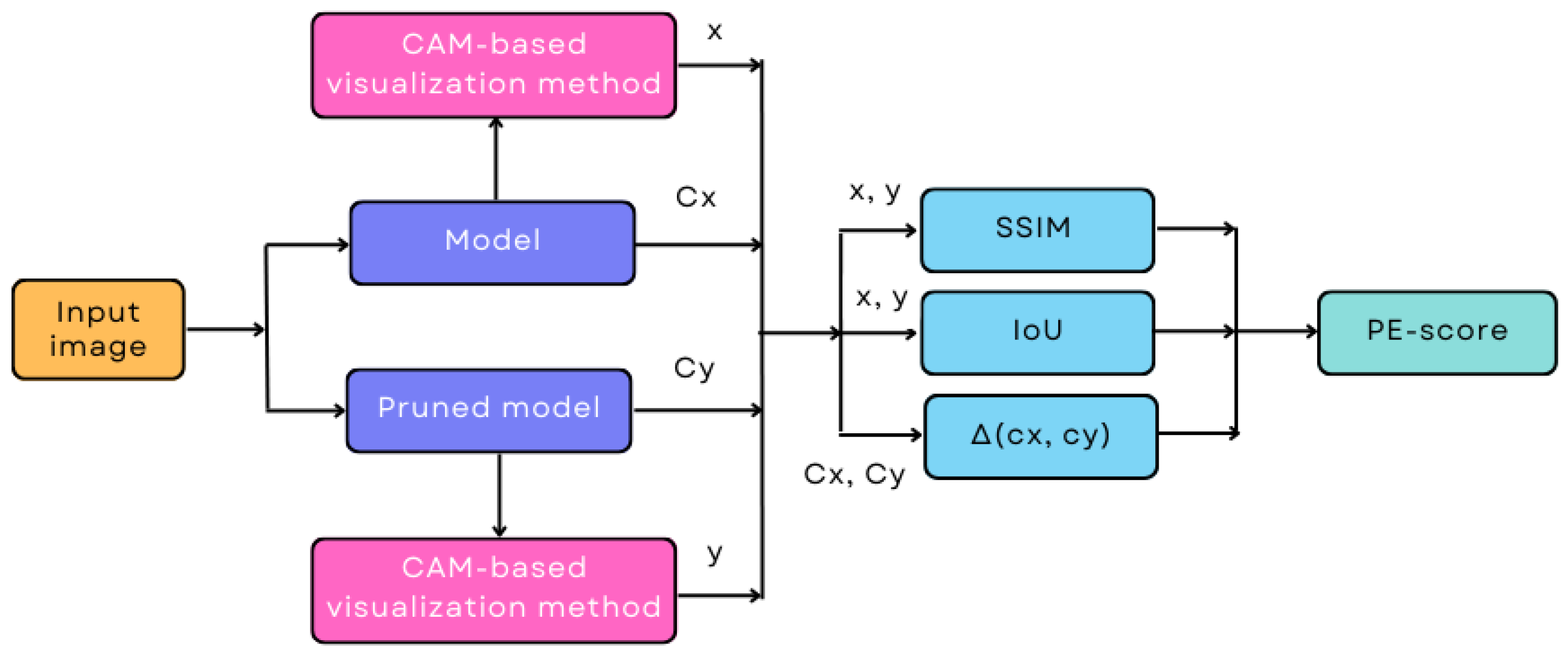
Figure 3 presents a general diagram for the computation of the PE-score.
Let us denote the heatmap of the original model as x and that of the pruned model as y. Then, the value of S S I M between the two images is calculated using Equation (2), as follows:
S S I M ( x , y ) = ( 2 μ x μ y + c 1 ) ( 2 σ x y + c 2 ) ( μ x 2 + μ y 2 + c 1 ) , ( σ x 2 + σ y 2 + c 2 ) ,
where μ x , σ x 2 , μ y and σ y 2 correspond to the local mean and variance of x and y, respectively, while σ x y is the covariance between x and y. On the other hand, c 1 and c 2 are two constants to stabilize the division.
From x and y, we calculate the binarized heatmaps by applying a threshold equal to the average of the heatmap pixels, yielding x b and y b , respectively. At the output, the white region corresponds to the highlighted pixels and the black region to the non-discriminative pixels. Then, I o U is calculated using Equation (3), as follows:
I o U ( x b , y b ) = O p U p ,
where O P and U P correspond to the overlapping white pixels and the union of the white pixels between x b and y b , respectively. It is important to note that, in this case, the I o U metric is used at the pixel level and not at the area level, as is usually done in object detection and segmentation.
Next, the confidence variation between the original and the pruned model is calculated. The confidence of the original model is defined as the probability of membership in the class estimated by the model, represented as c x , while the confidence of the pruned model is defined as c y . Then, the confidence variation ( Δ ) is obtained from Equation (4) as follows:
Δ ( c x , c y ) = m a x 0 , c x c y c x ,
With these three values, the PE-score per image of the test dataset is obtained using Equation (5), as follows:
P E = 3 1 S S I M ( x , y ) + ϵ + 1 I o U ( x b , y b ) + ϵ + 1 1 Δ ( c x , c y ) + ϵ
The third term of the denominator is 1 / ( 1 Δ + ϵ ) instead of 1 / ( Δ + ϵ ) , because Δ is inversely proportional to the PE-score. In the case of S S I M and I o U , they are directly proportional to the PE-score, so they are in the form of 1 / ( S S I M + ϵ ) and 1 / ( I o U + ϵ ) in the denominator of the PE-score. It is necessary to include the term ϵ , to avoid having indeterminate values in the divisions—for example, if S S I M = 0 . A very small value of ϵ is assumed, within the range of the PE-score—specifically, ϵ = 1 × 10 13 . In addition, the number three in the numerator corresponds to the number of metrics used to calculate the PE-score. A high PE-score implies that the model is highly trustworthy, which corresponds to high values of S S I M and I o U and a low value of Δ . For example, if x = y and x b = y b , then S S I M = 1 and I o U = 1 . Additionally, if c x = c y (i.e., the class membership values are the same in the two models), then Δ = 0 . Taking these three values into account, they are substituted into Equation (5), and we have P E = 3 / ( 1 + 1 + 1 ) = 3 / 3 = 1 . Then, as the PE-score approaches 1, the reliability of the pruned model increases. In a second case, if the most important filters are removed during the pruning process, then the patterns extracted by this model will not be the same as those for the original model, obtaining, for example, S S I M ( x , y ) = 0.4 and I o U ( x b , y b ) = 0.4 . Therefore, even if the image classification is still correct, the variation in confidence will not be zero, but, let us assume, Δ = 0.2 . Substituting these values into Equation (5), we obtain P E = 3 / ( 2.5 + 2.5 + 1.25 ) = 3 / 6.25 = 0.48 . This means that as the value of the PE-score approaches 0, the confidence in the pruned model decreases.
Finally, to obtain the PE-score of the model, the following steps are performed.
  • Calculate the PE-score for each image of each class of the test dataset. In particular, a P E k i is obtained, where k varies from 1 to the number of classes K, and i varies from 1 to the number of images of the specific class, i.e., M k .
  • Calculate the average PE-score per class, i.e., P E k ¯ = i = 1 M k P E k i M k
  • Weight the PE-score obtained by each class, taking into account its weight ( W k ) within the dataset, as follows: P E m o d e l = k = 1 K W k × P E k ¯ .
Suppose that the test dataset has 10 classes, i.e., K = 10 , and M k = [100, 50, 100, 100, 200, 50, 50, 100, 150, 100]; then, W k = [0.1, 0.05, 0.1, 0.1, 0.2, 0.05, 0.05, 0.1, 0.15, 0.1]. The PE-score value obtained for each class is then weighted by the corresponding W value.
In summary, the proposed metric can be used to measure the reliability of a pruned model. If the value is close to 1, it means that the patterns on which the pruned model bases its decision are very similar to those of the original model; otherwise, if the value is close to 0, it means that the filters that extract the representative patterns of the class have been removed, and therefore the new model is not reliable.
This metric can be calculated using any method used to visualize and interpret CNNs. However, it is important to clarify that the model trustworthiness threshold may vary depending on the CAM-based method used. This is because there may be differences in the highlighted pixels when using different visualization methods, or, in other words, some CAM-based methods are more accurate in identifying the area of interest in the model.

4. Results

In this section, we present the results of the impact of pruning on sequential CNN models, namely VGG11, for two image sets of different complexity (CIFAR10 and COVID-19), two pruning methods (SeNPIS-Faster and Weight) and three visualization methods (Grad-CAM, Grad-CAM++ and Ablation-CAM). First, a complexity analysis of the datasets used in this study is presented, using the complexity calculation criteria based on the work by [30]. Then, for each of the datasets, the results of the pruning impact are presented in terms of the proposed metric, the PE-score. From these results, the analysis between the accuracy of the pruned model and the obtained PE-score, as well as the dataset used, is presented in the Discussion section.

4.1. Complexity of the Dataset

To begin the results phase, the complexity of the two datasets selected in this study will be analyzed: CIFAR10 and COVID-19. To do so, we will apply a metric for the measurement of dataset complexity called CSG (Cumulative Spectral Gradient) by combining the probability product kernel and graph theory [30]. It has been shown that there is a strong correlation between the performance of the model and the CSG value, with the advantage that the level of difficulty of class separation can be known a priori before training the classification model. A low value (CSG = 0) indicates that the dataset is of low complexity, while a high value implies greater difficulty in separating the classes. An advantage of CSG over other state-of-the-art dataset complexity measures is that it has only two hyperparameters (M: number of classes, k: number of neighbors), and the separability results depend little on the value of the chosen hyperparameters.
Table 3 shows the CSG results on two benchmark datasets (MNIST and Fashion-MNIST), as well as on the two datasets selected for the present work. According to the literature, the accuracy for MNIST and CIFAR10 using ResNet is 99.68% and 95.55%, respectively (as reported in https://paperswithcode.com/sota/image-classification-on-mnist and https://paperswithcode.com/sota/image-classification-on-cifar-10, both URLs were accessed on 5 May 2023). This means that the complexity of CIFAR10 is higher than that of MNIST, which is consistent with that obtained with CSG, being significantly higher in CIFAR10 than in MNIST. Therefore, the complexity of the COVID-19 dataset is lower than that of CIFAR10 because its CSG is significantly lower.
Two datasets of different complexity were selected for the experimental phase in order to
  • Determine whether there is a direct relationship between the decrease in model accuracy and the decrease in PE-score as PR increases;
  • Determine why, in some datasets, there is a fluctuation in accuracy as PR increases and PE decreases.

4.2. Trustworthiness of Pruned Models: Case of the CIFAR10 Dataset

CIFAR10 is one of the most widely used datasets for computer vision using machine learning and deep learning models. It consists of 10 classes, namely airplane, automobile, bird, cat, deer, dog, frog, horse, ship and truck. For each class, there are six thousand 32 × 32 pixel color images. The dataset is divided (by default) into fifty thousand images for training and ten thousand images for testing (see https://www.cs.toronto.edu/~kriz/cifar.html for more information. This URL was accessed on 5 May 2023).
On the other hand, SENPIS-Faster is a reduced version of the method proposed by Pachón in 2022 [16], in which the “IS attenuation” module is disabled to obtain the pruned model in less time. Therefore, the accuracy results presented in this section may be slightly lower than those published for the original method (approximately 0.15% on average). In addition, the weight method based on the L2-norm is selected for this study. The purpose of using two pruning methods is to verify that the PE-score is directly related to the accuracy of the pruned model, i.e., to verify whether a lower PE means lower accuracy, regardless of the pruning method used.
First, the VGG11 network is trained with CIFAR10, for a total of 10 epochs, using the SGD optimizer and a batch size of 32. The model is then pruned with six uniform pruning rates (UPR = 35%, 50%, 70%, 80%, 88% and 96%), and then fine tuning with 10 epochs is applied. For each pruned model, the S S I M , I o U and confidence variance are computed for each of the images in each class, and the PE-score is obtained according to the procedure described in Section 3.
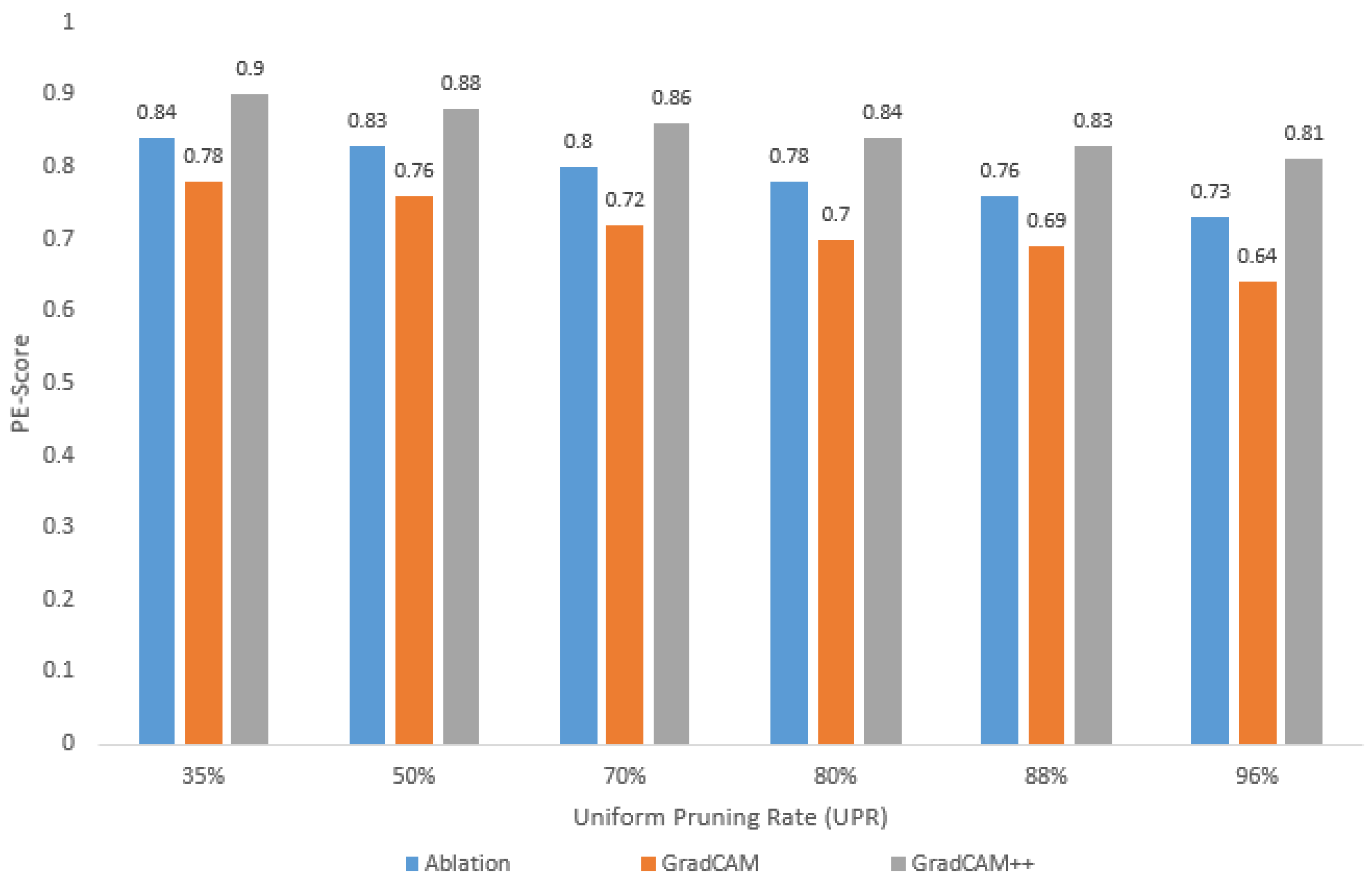
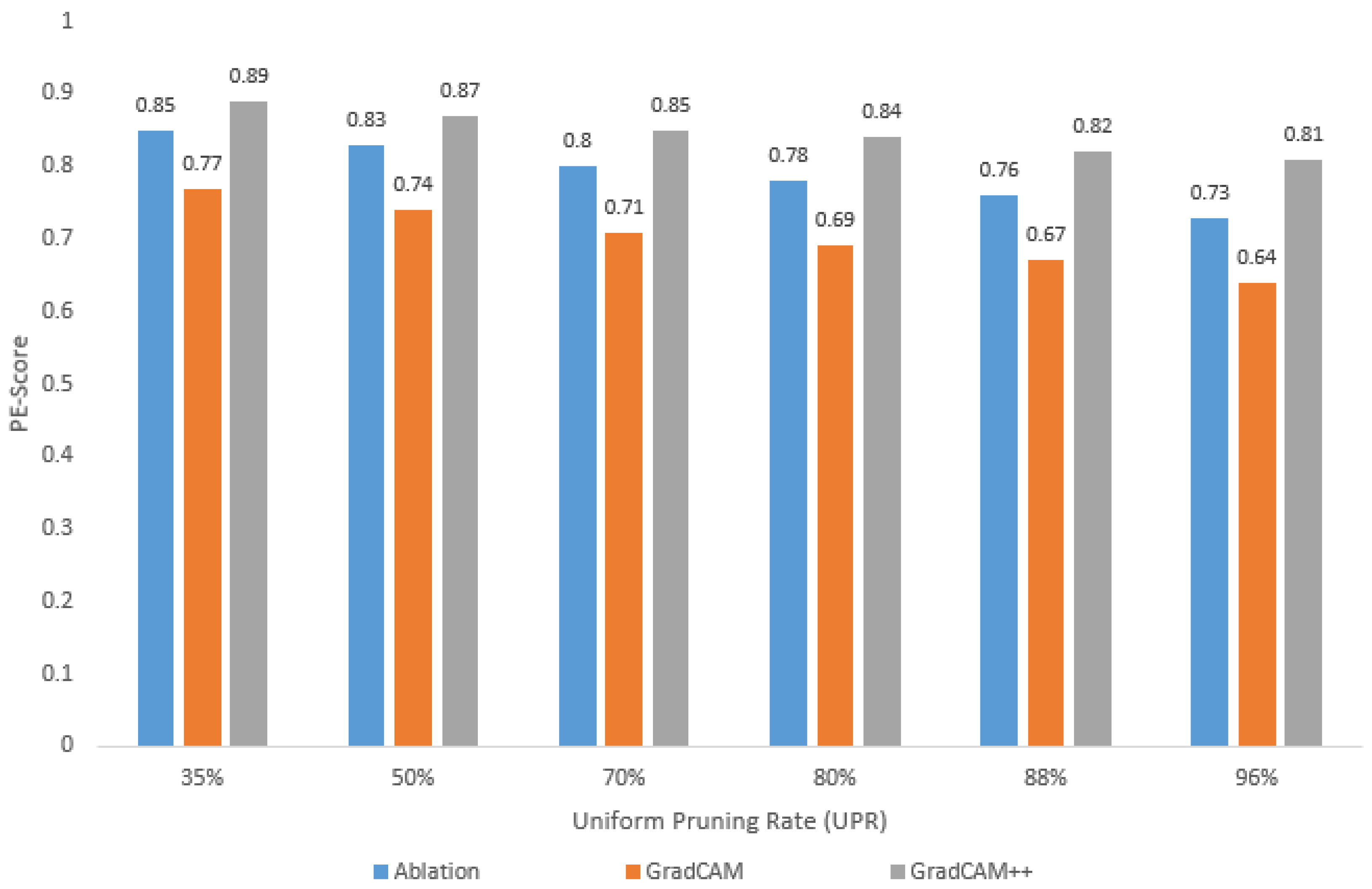
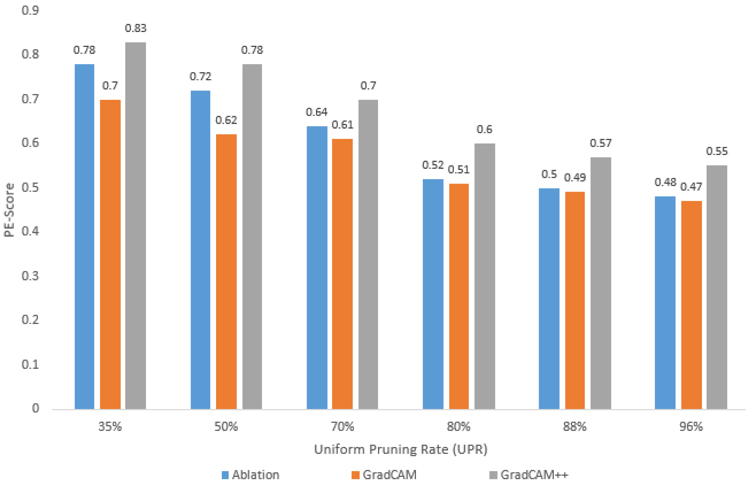
Figure 4 presents the results of the PE-score for six pruned models using SeNPIS-Faster and three visualization methods (Ablation, GradCAM and GradCAM++), and Figure 5 shows the corresponding results obtained using the weight pruning method.
The following comments can be made from the above graphs:
  • As the UPR increases, the PE-sore decreases, regardless of the visualization method selected for S S I M and I o U calculation;
  • For the different UPR values, the highest PE-score is obtained with GradCAM++, while the lowest value corresponds to GradCAM, i.e., depending on the visualization method used, the PE-score varies for the same pruned model;
  • Using GradCAM++, a loss in accuracy of less than 1% implies a PE-score greater than 0.87 (in this case, a UPR of up to 50%);
  • Using GradCAM++, a loss in accuracy of around 10% implies a PE-score around 0.81 (in this case, a UPR = 96%).
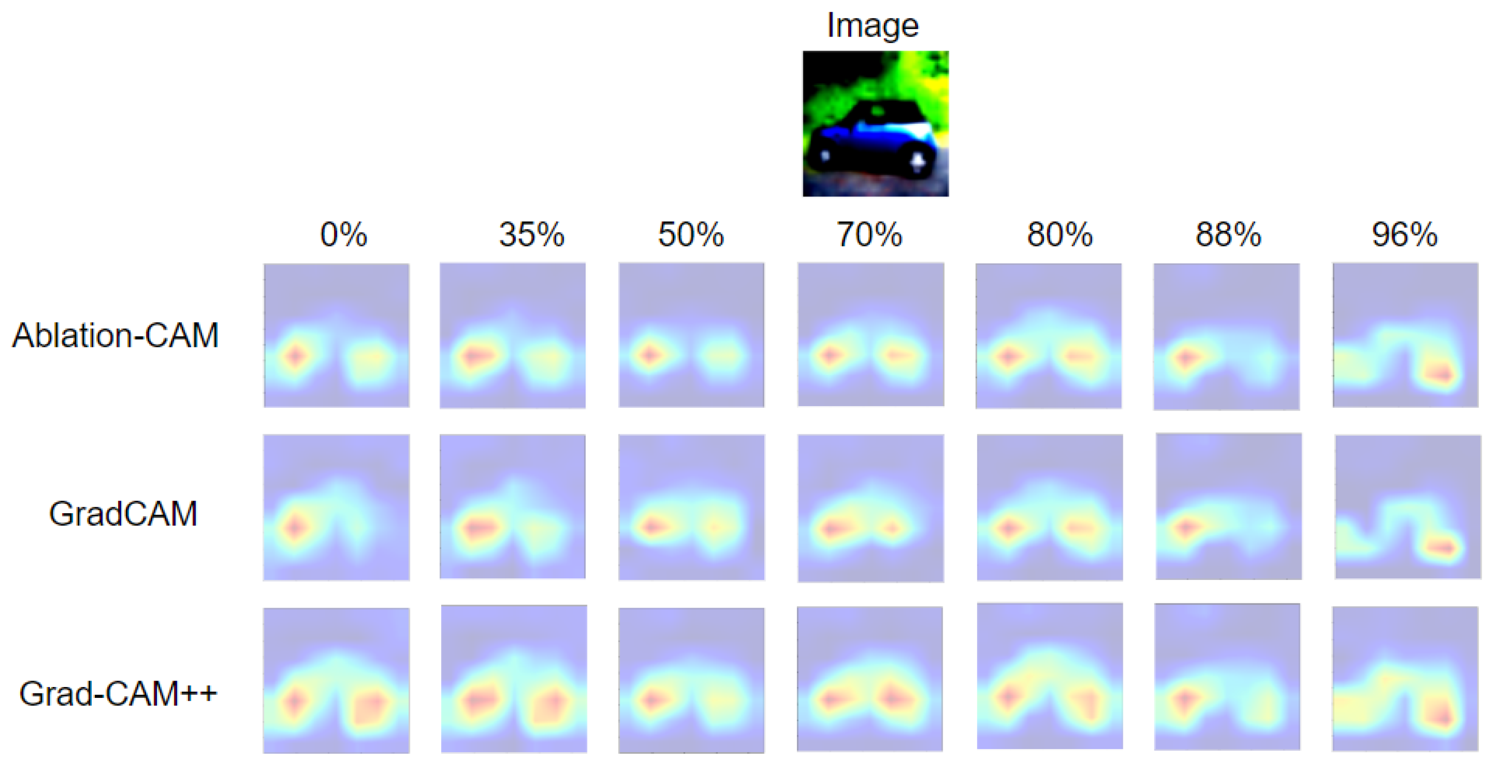
Next, Figure 6 shows the explanation maps of unpruned and pruned models with SeNPIS-Faster, for six UPR values and three visualization methods (Ablation-CAM, CAM, Grad-CAM++).
As shown in Figure 6, the pixels that identify the unpruned model to determine the car class correspond to the tires. As the UPR value increases, the pruned model continues to focus mostly on the same pixels as the unpruned model, but the intensity of its activation decreases slightly. For example, the high-intensity area (red color) of the left tire of the car becomes medium-intensity (yellow color) when UPR = 96% and the visualization method is Grad-CAM++. In addition, it can be observed that for the same network, input image and UPR value, the Grad-CAM++ method is the one that best identifies the pixels belonging to the class (the most representative ones). For this reason, the PE-score obtained using Grad-CAM++ is superior to that with the other two methods.

4.3. Trustworthiness of Pruned Models: Case of the COVID-19 Dataset

In this section, we present results using a healthcare dataset called COVID-19, which is available from the IEEE DataPort (https://ieee-dataport.org/documents/covid-19dataset, accessed on 1 February 2023). This dataset contains three classes: healthy, pneumonia and Covid. The images are grayscale with 256 × 256 pixels. The total number of images per class is 982, 1104 and 982, respectively.
Similar to the previous case study, we train a VGG-11 network with 10 epochs, SGD as the optimizer and a batch size of 32. The trained model is then pruned using two methods (SeNPIS-Faster and weight), with six uniform rates (35%, 50%, 70%, 80%, 88% and 96%), and fine tuned with 10 epochs. Again, the objective is not to compare which pruning method is better but to determine whether there is a relationship between the accuracy of the pruned model and its PE-score (which is obtained as described in Section 3).
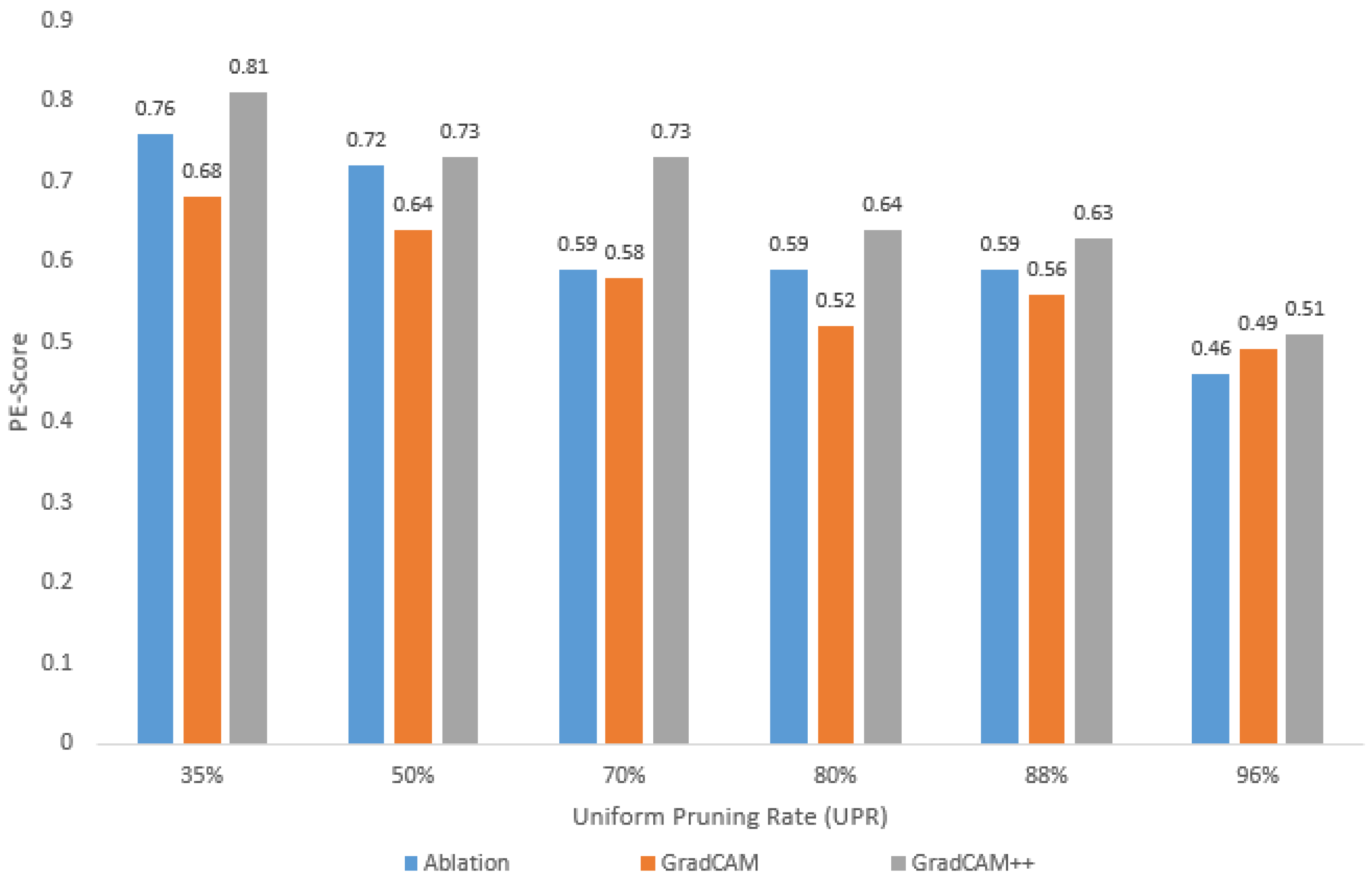
Figure 7 presents the results of the PE-score for six pruned models using weight and three visualization methods (Ablation, GradCAM and GradCAM++).
An unexpected result emerges in this dataset (see Figure 7). As the UPR increases, the PE-score decreases (as in the case of CIFAR10), but the accuracy of the pruned model does not necessarily decrease as the UPR increases. For example, when the UPR is 35% or 50%, the accuracy is higher than that of the unpruned model, even though the PE-score decreases. The question then arises of whether this atypical fluctuating behavior for the accuracy occurs only for models pruned with the weight method or also when another pruning method is used. Therefore, we check the results for SeNPIS-Faster (see Figure 8).
Similar to the results obtained with the weight pruning method, in the case of SeNPIS-Faster (see Figure 8), the accuracy values of the pruned model are higher than those of the unpruned model, even when the UPR increases and the PE-score decreases. For example, at a very high UPR of 88%, the accuracy of the pruned model exceeds that of the unpruned model by 1.31% (i.e., a c c b a s e l i n e = 96.08 % ; a c c U P R = 88 % = 97.39 % ), even though the PE-score decreases significantly (i.e., P E b a s e l i n e = 1 ; P E U P R = 88 % = 0.63 % ). This means that the new pruned model focuses on different patterns than the original model, which may lead to an increase in the hit rate. Therefore, in such cases, it is necessary to verify whether the new patterns extracted by the pruned model are representative of the class or, on the contrary, are distractors from the image set (other types of objects, significant changes in image brightness or background, etc.).
Figure 9 shows the explanation maps for an image from the COVID-19 dataset, using SeNPIS-Faster for the pruned models with six UPR values. Unlike the results obtained for the CIFAR10 dataset, the pixels activated after increasing the UPR value change significantly with respect to the pixels activated in the unpruned model. In other words, the model focuses on a different area of the image for decision making, which could be a “distractor” in the dataset and does not correspond to the representative patterns of the class. For this reason, if there are fluctuations in the PE-score value as the UPR increases, it is necessary to check the activation maps to verify the confidence of the pruned model, and to not only rely on the accuracy of the model as an indicator of its quality.

5. Discussion

The goal of this paper was to propose a metric to determine the trustworthiness of a pruned model that moves beyond assessing the model’s success in image classification with conventional metrics such as the accuracy or F1-score. Specifically, we wished to show that the proposed metric, called the PE-score, can be used to determine whether a pruned model is reliable and at which value of the PR (pruning rate) it is no longer trustworthy. For this purpose, an exhaustive study was performed with two datasets of different complexity (CIFAR10 and COVID-19), two pruning methods (Weight and SeNPIS-Faster) and six uniform pruning rates (UPR = 35%, 50%, 70%, 80%, 88%, 96%). All pruned models were fine tuned under the same number of epochs, optimizer and learning rate, so that the results were comparable.
In the first dataset, CIFAR10, it was found that with the two pruning methods used, both the model accuracy and the PE-score decreased as the UPR increased. For UPR values up to 50%, the accuracy decreased by up to 1%, corresponding to a PE-score of at least 0.87 (Grad-CAM++ used), whereas, for UPR values above 50%, the accuracy could decrease by more than 10%, with a PE-score of approximately 0.8 (Grad-CAM++ used). Examining the explanation maps obtained with Grad-CAM++, it can be seen that the patterns (pixels) activated in the pruned models with a UPR of 30% or 50% were similar (in shape and intensity) to those of the unpruned model, whereas, for UPR values above 50%, the intensity of activation decreased significantly with respect to that of the unpruned model. Thus, the PE-score allows us to determine the reliability of the pruned model, bearing in mind that a value close to 1 is sufficient to verify that the pruned model behaves very similarly to the unpruned model.
On the other hand, with the COVID-19 dataset, it was found that there was no direct relationship between the accuracy of the pruned model and its PE-score, since, as the UPR increased, the PE-score of the pruned model decreased, but its accuracy showed a fluctuating behavior. When the explanation maps obtained with the three visualization methods (Ablation-CAM, Grad-CAM and Grad-CAM++) were examined, it was found that as the UPR increased, the area of the image that was activated changed significantly with respect to that of the unpruned model, which could focus on distractors or incorrect patterns in the class. This dataset demonstrates the importance of having a metric to evaluate the pruned model, in addition to accuracy or a similar metric based on the model’s hits, in order to determine whether or not the pruned model is reliable. Specifically, this dataset could be used to show that the high accuracy of the pruned model does not mean that it is reliable with respect to the unpruned model.
Finally, from the PE-score results per dataset and UPR value, it can be observed that the PE-score values obtained using the Grad-CAM++ visualization method are higher than those obtained using the Grad-CAM and Ablation-CAM methods. Thus, the PE-score value that guarantees the high reliability of the pruned model depends on the chosen visualization method.
In general, it is suggested to use the following procedure to determine up to which PR (pruning rate) value the pruned model can be trusted.
  • Train the network on the dataset to be classified, obtaining the unpruned model.
  • Prune the model with a low PR value. It can be uniform (UPR) or adaptive (APR). Measure the accuracy of the pruned model and the PE-score, taking into account what is described in Section 3 of this paper.
  • Repeat step 2 with different values of PR. In all cases, use the same fine-tuning hyperparameters (e.g., epochs, optimizer, learning rate). Calculate the PE-score and the accuracy value for each PR value.
  • Check that both the PE-score and accuracy decrease as the PR increases. If so, select the PR value at which the model drops to 1% (or the accuracy reduction criterion for the selected application).
  • Otherwise, if the accuracy has a fluctuating behavior (e.g., increases, decreases, increases) as the PR increases and the PE-score decreases, then it is mandatory to check the explanation maps for each of the PR values. The maximum PR for which the pruned model can be trusted is the one for which its explanation map is very similar to that of the unpruned model.
In summary, it is not possible to recommend a “universal value” of PE that guarantees the reliability of the model, since it is highly dependent on both the dataset type (e.g., complexity, quality) and the visualization method used for the explanation maps.

6. Conclusions

This paper proposes a metric, called the PE-score, to evaluate the reliability of pruned models, based on a comparison between the explanation maps of the unpruned model and those of the pruned model, as well as the confidence in the class. According to the results obtained in the experimental phase, it is observed that there is a strong relationship between the PE-score and the accuracy of the pruned model as the PR (pruning rate) increases. A high PE-score (for example, around 0.9) ensures that the pruned model focuses on the pixels (patterns) as the original model, while, as the PE-score decreases, the CAM-highlighted areas change or their intensity decreases. However, if the dataset contains distractors, the pruned model may focus on different pixels to the unpruned model and may even increase its accuracy at high PR values. In these cases, the PE-score will decrease as the PR increases, helping to identify this type of behavior.
The experiments carried out show that metrics such as accuracy do not allow us to measure the reliability of pruned models, and that it is necessary to use metrics other than those based on classification hits to adequately measure the behavior of the pruned model, as the proposed PE-score does.

Author Contributions

Conceptualization, C.G.P. and D.B.; Methodology, D.R. and D.B.; Software, C.G.P.; Validation, C.G.P.; Formal analysis, C.G.P. and D.B.; Investigation, D.R.; Writing—original draft, D.B. and C.G.P.; Writing—review and editing, D.R.; Supervision, D.B. and D.R.; Funding acquisition, D.B. and D.R. All authors have read and agreed to the published version of the manuscript.

Funding

This work has been sponsored by the Universidad Militar Nueva Granada— Vicerrectoría de investigaciones, with the project INV-ING-3786, entitled “Compression of deep learning models for image classification tasks applied to industry 4.0”.

Data Availability Statement

Not applicable.

Conflicts of Interest

The authors declare no conflict of interest.

Abbreviations

The following abbreviations are used in this manuscript:
CNNConvolutional Neural Network
ACCAccuracy
APRAdaptive Pruning Rate
UPRUniform Pruning Rate
PRPruning Rate
PEPruning Efficiency
NNNeural Network

References

  1. Liang, T.; Glossner, J.; Wang, L.; Shi, S.; Zhang, X. Pruning and quantization for deep neural network acceleration: A survey. Neurocomputing 2021, 461, 370–403. [Google Scholar] [CrossRef]
  2. Marinó, G.C.; Petrini, A.; Malchiodi, D.; Frasca, M. Deep neural networks compression: A comparative survey and choice recommendations. Neurocomputing 2023, 520, 152–170. [Google Scholar] [CrossRef]
  3. Alqahtani, A.; Xie, X.; Jones, M.W. Literature review of deep network compression. Informatics 2021, 8, 77. [Google Scholar] [CrossRef]
  4. Li, H.; Kadav, A.; Durdanovic, I.; Samet, H.; Graf, H.P. Pruning filters for efficient convnets. In Proceedings of the 5th International Conference on Learning Representations (ICLR), Toulon, France, 24–26 April 2017. [Google Scholar]
  5. Kumar, A.; Shaikh, A.M.; Li, Y.; Bilal, H.; Yin, B. Pruning filters with L1-norm and capped L1-norm for CNN compression. Appl. Intell. 2021, 51, 1152–1160. [Google Scholar] [CrossRef]
  6. He, Y.; Kang, G.; Dong, X.; Fu, Y.; Yang, Y. Soft filter pruning for accelerating deep convolutional neural networks. arXiv 2018, arXiv:1808.06866. [Google Scholar]
  7. He, Y.; Liu, P.; Wang, Z.; Hu, Z.; Yang, Y. Filter pruning via geometric median for deep convolutional neural networks acceleration. In Proceedings of the IEEE/CVF Conference on Computer Vision and Pattern Recognition, Long Beach, CA, USA, 15–20 June 2019; pp. 4340–4349. [Google Scholar]
  8. Molchanov, P.; Tyree, S.; Karras, T.; Aila, T.; Kautz, J. Pruning convolutional neural networks for resource efficient inference. In Proceedings of the 5th International Conference on Learning Representations (ICLR), Toulon, France, 24–26 April 2017. [Google Scholar]
  9. Sun, X.; Ren, X.; Ma, S.; Wang, H. meprop: Sparsified back propagation for accelerated deep learning with reduced overfitting. In Proceedings of the International Conference on Machine Learning, PMLR, Sydney, Australia, 6–11 August 2017; pp. 3299–3308. [Google Scholar]
  10. Liu, C.; Wu, H. Channel pruning based on mean gradient for accelerating convolutional neural networks. Signal Process. 2019, 156, 84–91. [Google Scholar] [CrossRef]
  11. Joo, D.; Baek, S.; Kim, J. Which Metrics for Network Pruning: Final Accuracy? Or Accuracy Drop? In Proceedings of the 2022 IEEE International Conference on Image Processing (ICIP), Bordeaux, France, 16–19 October 2022; IEEE: Piscataway, NJ, USA, 2022; pp. 1071–1075. [Google Scholar] [CrossRef]
  12. Luo, J.H.; Zhang, H.; Zhou, H.Y.; Xie, C.W.; Wu, J.; Lin, W. Thinet: Pruning cnn filters for a thinner net. IEEE Trans. Pattern Anal. Mach. Intell. 2018, 41, 2525–2538. [Google Scholar] [CrossRef] [PubMed]
  13. Zhao, C.; Ni, B.; Zhang, J.; Zhao, Q.; Zhang, W.; Tian, Q. Variational convolutional neural network pruning. In Proceedings of the IEEE/CVF Conference on Computer Vision and Pattern Recognition, Long Beach, CA, USA, 15–20 June 2019; pp. 2780–2789. [Google Scholar]
  14. Li, Q.; Li, H.; Meng, L. Feature map analysis-based dynamic cnn pruning and the acceleration on fpgas. Electronics 2022, 11, 2887. [Google Scholar] [CrossRef]
  15. Krizhevsky, A.; Hinton, G. Learning Multiple Layers of Features from Tiny Images; University of Toronto: Toronto, ON, Canada, 2009. [Google Scholar]
  16. Pachón, C.G.; Ballesteros, D.M.; Renza, D. SeNPIS: Sequential Network Pruning by class-wise Importance Score. Appl. Soft Comput. 2022, 129, 109558. [Google Scholar] [CrossRef]
  17. Yeom, S.K.; Seegerer, P.; Lapuschkin, S.; Binder, A.; Wiedemann, S.; Müller, K.R.; Samek, W. Pruning by explaining: A novel criterion for deep neural network pruning. Pattern Recognit. 2021, 115, 107899. [Google Scholar] [CrossRef]
  18. Yang, C.; Liu, H. Channel pruning based on convolutional neural network sensitivity. Neurocomputing 2022, 507, 97–106. [Google Scholar] [CrossRef]
  19. Chen, Z.; Liu, C.; Yang, W.; Li, K.; Li, K. LAP: Latency-aware automated pruning with dynamic-based filter selection. Neural Netw. 2022, 152, 407–418. [Google Scholar] [CrossRef] [PubMed]
  20. He, Y.; Zhang, X.; Sun, J. Channel pruning for accelerating very deep neural networks. In Proceedings of the IEEE International Conference on Computer Vision, Venice, Italy, 22–29 October 2017; pp. 1389–1397. [Google Scholar]
  21. Ding, X.; Ding, G.; Guo, Y.; Han, J.; Yan, C. Approximated oracle filter pruning for destructive cnn width optimization. In Proceedings of the International Conference on Machine Learning, PMLR, Beach, CA, USA, 9–15 June 2019; pp. 1607–1616. [Google Scholar]
  22. Gamanayake, C.; Jayasinghe, L.; Ng, B.K.K.; Yuen, C. Cluster pruning: An efficient filter pruning method for edge ai vision applications. IEEE J. Sel. Top. Signal Process. 2020, 14, 802–816. [Google Scholar] [CrossRef] [Green Version]
  23. Chattopadhay, A.; Sarkar, A.; Howlader, P.; Balasubramanian, V.N. Grad-cam++: Generalized gradient-based visual explanations for deep convolutional networks. In Proceedings of the 2018 IEEE Winter Conference on Applications of Computer Vision (WACV), Lake Tahoe, NV, USA, 12–15 March 2018; IEEE: Piscataway, NJ, USA, 2018; pp. 839–847. [Google Scholar] [CrossRef] [Green Version]
  24. Canziani, A.; Paszke, A.; Culurciello, E. An analysis of deep neural network models for practical applications. arXiv 2016, arXiv:1605.07678. [Google Scholar]
  25. Ghimire, D.; Kil, D.; Kim, S.H. A Survey on Efficient Convolutional Neural Networks and Hardware Acceleration. Electronics 2022, 11, 945. [Google Scholar] [CrossRef]
  26. Zhou, B.; Khosla, A.; Lapedriza, A.; Oliva, A.; Torralba, A. Learning deep features for discriminative localization. In Proceedings of the IEEE Conference on Computer Vision and Pattern Recognition, Las Vegas, NV, USA, 27–30 June 2016; pp. 2921–2929. [Google Scholar]
  27. Selvaraju, R.R.; Cogswell, M.; Das, A.; Vedantam, R.; Parikh, D.; Batra, D. Grad-cam: Visual explanations from deep networks via gradient-based localization. In Proceedings of the IEEE International Conference on Computer Vision, Venice, Italy, 22–29 October 2017; pp. 618–626. [Google Scholar]
  28. Desai, S.S.; Ramaswamy, H.G. Ablation-cam: Visual explanations for deep convolutional network via gradient-free localization. In Proceedings of the IEEE/CVF Winter Conference on Applications of Computer Vision, Snowmass Village, CO, USA, 1–5 March 2020; pp. 983–991. [Google Scholar]
  29. Ballesteros, D.M.; Rodriguez-Ortega, Y.; Renza, D.; Arce, G. Deep4SNet: Deep learning for fake speech classification. Expert Syst. Appl. 2021, 184, 115465. [Google Scholar] [CrossRef]
  30. Branchaud-Charron, F.; Achkar, A.; Jodoin, P.M. Spectral metric for dataset complexity assessment. In Proceedings of the IEEE/CVF Conference on Computer Vision and Pattern Recognition, Long Beach, CA, USA, 15–20 June 2019; pp. 3215–3224. [Google Scholar]
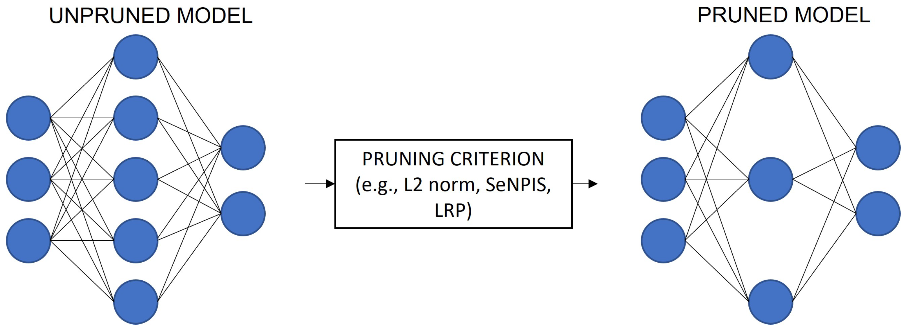
Figure 1. Example of pruning of NNs, with PR = 40%.
Bdcc 07 00111 g001
Figure 2. Example images of explanatory maps generated by Ablation-CAM, GradCAM and Grad-CAM++. Dataset: CIFAR10. Network: VGG11. Optimizer: SGD with momentum. Learning rate = 0.001. Batch size = 32.
Bdcc 07 00111 g002
Figure 3. General scheme for calculation of the reliability of the pruned model. This process is performed for each image of each class and is applied to all classes. x and y correspond to the heatmaps of the input image obtained from the original model and the pruned model, respectively; c x and c y correspond to the confidence of the original model and the pruned model, respectively; and S S I M is the structural similarity between the two heatmaps. I o U is a measure of the pixel-to-pixel similarity of the two heatmaps, and Δ ( c x , c y ) is the confidence variance between the two models.
Bdcc 07 00111 g003
Figure 4. CIFAR10 dataset: PE-scores of pruned models with the SeNPIS-Faster method, six UPRs (Uniform Pruning Rates) and three visualization methods (Ablation, GradCAM and GradCAM++). The higher the value of PE, the more reliable the pruned model (i.e., it focuses on the same patterns as the original model). The accuracy in each case is as follows: a c c b a s e l i n e = 92.8 % ; a c c U P R = 35 % = 92.22 % ; a c c U P R = 50 % = 92.09 % ; a c c U P R = 70 % = 89.35 % ; a c c U P R = 80 % = 89.17 % ; a c c U P R = 88 % = 86.30 % ; a c c U P R = 96 % = 81.91 % .
Bdcc 07 00111 g004
Figure 5. CIFAR10 dataset: PE-scores of pruned models with the Weight method, six UPRs (Uniform Pruning Rates) and three visualization methods (Ablation, GradCAM and GradCAM++). The higher the value of PE, the more reliable the pruned model, i.e., it focuses on the same patterns as the original model. The accuracy in each case is as follows: a c c b a s e l i n e = 92.8 % ; a c c U P R = 35 % = 92.55 % ; a c c U P R = 50 % = 92.26 % ; a c c U P R = 70 % = 89.43 % ; a c c U P R = 80 % = 88.33 % ; a c c U P R = 88 % = 87.85 % ; a c c U P R = 96 % = 82.48 % .
Bdcc 07 00111 g005
Figure 6. Visual explanation maps of unpruned model (i.e., UPR = 0%) and six pruned models (UPR = 35%, 50%, 70%, 80%, 88% and 96%). Dataset: CIFAR10. Pruning method: SeNPIS-Faster. Visualization methods: Ablation-CAM, GradCAM and Grad-CAM++. Network: VGG11. Optimizer: SGD. Batch size = 32. Epochs (training) = 10, epochs (fine tuning) = 10.
Bdcc 07 00111 g006
Figure 7. COVID-19 dataset: PE-scores of pruned models with the Weight method, six UPRs (Uniform Pruning Rates) and three visualization methods (Ablation, GradCAM and GradCAM++). The higher the value of PE, the more reliable the pruned model, i.e., it focuses on the same patterns as the original model. The accuracy in each case is as follows: a c c b a s e l i n e = 96.08 % ; a c c U P R = 35 % = 97.39 % ; a c c U P R = 50 % = 97.55 % ; a c c U P R = 70 % = 94.13 % ; a c c U P R = 80 % = 96.08 % ; a c c U P R = 88 % = 92.99 % ; a c c U P R = 96 % = 94.78 % .
Bdcc 07 00111 g007
Figure 8. COVID-19 dataset: PE-scores of pruned models with the SeNPIS-Faster method, six UPRs (Uniform Pruning Rates) and three visualization methods (Ablation, GradCAM and GradCAM++). The higher the value of PE, the more reliable the pruned model, i.e., it focuses on the same patterns as the original model. The accuracy of each case is as follows: a c c b a s e l i n e = 96.08 % ; a c c U P R = 35 % = 97.06 % ; a c c U P R = 50 % = 96.90 % ; a c c U P R = 70 % = 96.08 % ; a c c U P R = 80 % = 96.25 % ; a c c U P R = 88 % = 97.39 % ; a c c U P R = 96 % = 94.94 % .
Bdcc 07 00111 g008
Figure 9. Explanation maps of unpruned model (i.e., UPR = 0%) and six pruned models (UPR = 35%, 50%, 70%, 80%, 88% and 96%). Dataset: COVID-19. Pruning method: SeNPIS-Faster. Visualization methods: Ablation-CAM, GradCAM and Grad-CAM++. Network: VGG11. Optimizer: SGD. Batch size = 32. Epochs (training) = 10, epochs (fine tuning) = 10.
Bdcc 07 00111 g009
Table 1. Comparison of representative state-of-the-art pruning methods. Evaluation criteria: accuracy, FLOPs reduction and parameter reduction. Network: VGG16. Dataset: CIFAR10.
MethodAccuracyFLOPs ReductionParameter Reduction
LRP [17]93.37%35.89%33.59%
Gradient [8]92.98%46.80%27.53%
Taylor [8]93.24%47.45%27.56%
Weight [4]93.31%24.47%44.49%
Variational [13]93.18%39.10%73.34%
SeNPIS [16]93.74%50.74%51.05%
Table 2. Comparison of representative state-of-the-art pruning methods. Evaluation criteria: accuracy drop and FLOPs reduction. Network: VGG16. Dataset: CIFAR10.
MethodAccuracy DropFLOPs Reduction
Channel pruning [18]0.01%42.9%
Channel pruning [18]0.53%54.1%
Channel pruning [18]1.46%65.8%
LAP [19]1.31%76.0%
Table 3. Comparison of CSG values for some image classification datasets.
DatasetAccuracy *CSGComplexity
MNIST99.68%0.1306Very low
COVID-1999.50%0.1938Very low
Fashion-MNIST96.91%0.5424Low
CIFAR1095.55%4.0676Medium
* According to the state-of-the-art.
Disclaimer/Publisher’s Note: The statements, opinions and data contained in all publications are solely those of the individual author(s) and contributor(s) and not of MDPI and/or the editor(s). MDPI and/or the editor(s) disclaim responsibility for any injury to people or property resulting from any ideas, methods, instructions or products referred to in the content.