Abstract
Developing a spiking neural network architecture that could prospectively be trained on energy-efficient neuromorphic hardware to solve various data analysis tasks requires satisfying the limitations of prospective analog or digital hardware, i.e., local learning and limited numbers of connections, respectively. In this work, we compare two methods of connectivity reduction that are applicable to spiking networks with local plasticity; instead of a large fully-connected network (which is used as the baseline for comparison), we employ either an ensemble of independent small networks or a network with probabilistic sparse connectivity. We evaluate both of these methods with a three-layer spiking neural network, which are applied to handwritten and spoken digit classification tasks using two memristive plasticity models and the classical spike time-dependent plasticity (STDP) rule. Both methods achieve an F1-score of 0.93–0.95 on the handwritten digits recognition task and 0.85–0.93 on the spoken digits recognition task. Applying a combination of both methods made it possible to obtain highly accurate models while reducing the number of connections by more than three times compared to the basic model.
1. Introduction
Neural network-based intelligent systems are widely employed in a wide range of tasks, from natural language processing to computer vision and signal processing. In edge computing, however, the use of deep learning methods still poses a variety of challenges, including latency and power consumption constraints, both during training and inference.
Neuromorphic computing devices, in which the information is encoded and processed in the form of binary events called spikes, offer a prospective solution to these problems. Modern neuroprocessors, e.g., TrueNorth [1], Loihi [2], or Altai https://motivnt.ru/neurochip-altai (accessed 8 February 2024), have been shown to achieve power consumption at the order of milliwatts [3]. Thus, these devices offer a powerful inference interface, and they can be used to deploy spiking neural networks (SNNs), thereby allowing both inference and training directly on the neurochip. This can be extremely useful for edge computing applications by reducing power consumption and latency.
In turn, memristor-based training poses its own unique set of challenges and limitations. The most prominent one arises from the hardware implementation of synapses, where every neuron can have only a limited amount of synapses [4,5,6], thus imposing limitations on the number of weights that a given network may have. In this regard, sparsely connected spiking networks, where the connectivity can be reduced depending on the hardware specifications, are a plausible solution.
In this study, we compared two methods of reducing connectivity in memristive spiking neural networks: a bagging ensemble of spiking neural networks and a probabilistic sparse SNN. Using a three-layer SNN with inhibitory and excitatory synapses, we solved the handwritten and spoken digits classification tasks, as well as compared the outcomes for the proposed connectivity reduction types and three plasticity models. The main contributions of this work are as follows:
- –
- We design a probabilistic sparse connectivity approach to creating a two-layer spiking neural network (achieved by implementing a bagging ensemble of two-layer SNNs) and then compare these two methods.
- –
- We propose an efficiency index that facilitates comparisons between different methods of connectivity reduction, and we will look to apply it to the SNNs used in the study.
- –
- We demonstrate that both connectivity reduction methods achieve competitive results on handwritten and spoken digit classification tasks, and that it can be used with the memristive plasticity models.
- –
- We show that the model that uses both connectivity reduction techniques simultaneously outperforms both methods in terms of the accuracy-per-connection efficiency metric.
The rest of the study is structured as follows: In Section 2, we provide a brief overview of the existing connectivity reduction methods for SNNs. In Section 3, we describe the datasets we use, the plasticity models, the base spiking neural structure, and the sparsity methods (which we utilized for comparison). In Section 4, we provide the accuracy estimations for the proposed approaches and discuss the obtained results in Section 5. Finally, we detail our conclusions in Section 6.
2. Literature Review
Connectivity reduction concerning spiking and artificial neural networks has been studied in several existing works.
A number of works have proposed to use a probabilistic coefficient to form connections between neurons in a spiking neural network. For example, the work of [7] used a network that consists of three layers of neurons. The first layer is responsible for encoding the input samples (images) into Poisson spike sequences. The second layer consists of 4000 excitatory and 1000 inhibitory leaky integrate and fire neurons. The output layer also consists of LIF neurons, the number of which corresponds to the number of classes in the selected dataset (EMNIST [8], YALE [9], or ORL [10]). The connections within the second layer are formed in accordance with the selected probability of 0.2. In this case, the weights of the synapses change depending on the spatial location of neurons and the dynamics of spike activity. The connections between the encoding layer and the second layer of neurons are excitatory without exhibiting plasticity. Probabilistic linking and changing weights using spatial location can achieve high classification accuracy on the image datasets.
Another approach to connectivity reduction that is present in the literature is based on designing locally connected SNNs, the weights in which are created in a sparse fashion according to a certain rule. In [11], for example, a routing scheme that used a hybrid of short-range direct connectivity and an address event representation network was developed. Without providing any benchmark results, the authors focused on the details of mapping a given SNN to the proposed architecture, and they showed that it yielded up to a 90% reduction in connectivity. The authors of the [12] study proposed a way through which to reduce connectivity in a three-layer network operating on the Winner Takes All principle. The input image, encoded by the first layer using frequency coding, was divided into small fragments that were then sent to individual neurons in the excitation layer. This made it possible to reduce the number of connections with local plasticity by up to 50% while maintaining the accuracy on the MNIST dataset at approximately 90%. The authors of [13] proposed a joined connectivity and weight learning approach inspired by the synapse elimination and synaptogenesis in biological neurons. The gradient in this work was redefined as an additional synaptic parameter, thereby facilitating a better adaptation of the network topology. A multilayer convolutional SNN trained using a surrogate gradient approach and pruned according to the designed method demonstrated an accuracy of about 89 and 92%, with less than 5% connectivity in the whole SNN for the MNIST and CIFAR datasets, respectively. Increasing the proportion of connectivity to 40% improved the quality of solving classification problems to 98.9 and 92.8%. The possibility of a sharp decrease in the number of connections can be caused by a large number of layers and neurons in the original network. Overall, this work demonstrates the fundamental applicability of the approaches used in classical machine learning for spiking neural networks.
In [14], a two-stage pruning method for on-chip SNNs was developed. The pruning was first performed during training based on weight update history and spike timing. After training, it was then via weight thresholding. By training a deep SNN with time-to-first-spike coding using the proposed approach, the authors decreased latency by a factor of 2 and reduced the network connectivity by 92% without accuracy loss. Another example can be found in [15], where the authors used a method of zeroing weights above a given threshold and achieved a 70% reduction in connectivity. In this paper, the network consists of a mixture of formal and spiking convolutional layers, and the resulting sparse hybrid network achieved more than 71% accuracy on the IVS 3cls [16] dataset. In [17], sparsity in a multilayer convolutional spiking network is achieved by limiting the number of connections associated with each neuron, and this is based on calculating the contribution of a neuron to the operation of the entire network. The proposed approach is shown to achieve high accuracy on such classical datasets as DVS-Gesture [18] (98%), MNIST (99%), CIFAR-10 (94%), and N-MNIST [19] (99%), with a 50% reduction in the number of connections. Finally, in [20], a sparse SNN topology was proposed, where the connectivity reduction was performed via a combination of pruning and quantization based on the power law weight-dependent plasticity model. Connectivity reduction was performed based on a threshold value at which the weights become zero. After training, the three-layer, fully connected SNN designed in the study achieved a classification accuracy of 92% on the MNIST dataset.
Thus, currently employed methods of reducing the connectivity in spiking neural networks are mostly encompassed by pruning, quantization, and local connectivity. However, ensemble learning, where multiple smaller networks are used together to form a stronger classifier, can be also viewed as a single sparse network. In this work, we explored this path to connectivity reduction and compared it to a probabilistic, locally connected SNN topology that was proposed in the work of [21], and which was investigated in our previous research with different types of plasticity models [22,23,24].
3. Materials and Methods
3.1. Datasets and Preprocessing
To train and evaluate the proposed methods, we used two benchmark datasets: the scikit-learn Digits (Digits) [25] and Free Spoken Digits Dataset (FSDD) [26]. The first consists of 1797 images of handwritten numbers, and the second contains 3000 audio recordings of spoken numbers from 0 to 9 in English. The choice of these datasets over larger and more widely used classification datasets such as MNIST, CIFAR-10, or N-MNIST was motivated by computational requirements. The training process for spiking neural networks when using local plasticity rules requires extensive computational experiments to select the combination of hyperparameters. We automated this process (see Section 4 for details), thereby placing a limit on the time required to train the network. The Digits dataset was quite difficult in comparison to MNIST due to containing less information about the handwritten digits in terms of image size and dataset volume (see the examples in Figure 1).
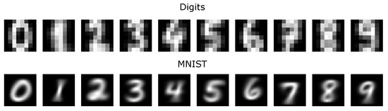
Figure 1.
Averaged samples by each class of handwritten digits from the Digits and MNIST datasets.
Both datasets had 10 classes, which could be broken down as 180 samples per class for Digits and 300 samples per class for FSDD. Additionally, the samples in FSDD varied by speaker as follows: 6 speakers in total and 50 recordings for each digit per speaker with different intonations.
The raw data were preprocessed as follows:
- (1)
- Feature representation: For Digits, their original vector representation in the form of pixel intensities was used without changes; for FSDD, a vector representing an audio sample was obtained by splitting the audio into frames, which was achieved by extracting 30 Mel-frequency cepstral coefficients [27] (MFCCs) and then averaging them across frames.
- (2)
- Normalization: Depending on the type of plasticity, the input vectors were normalized either by reducing to a zero mean and one standard deviation (standard scaling) or by L2 normalization.
- (3)
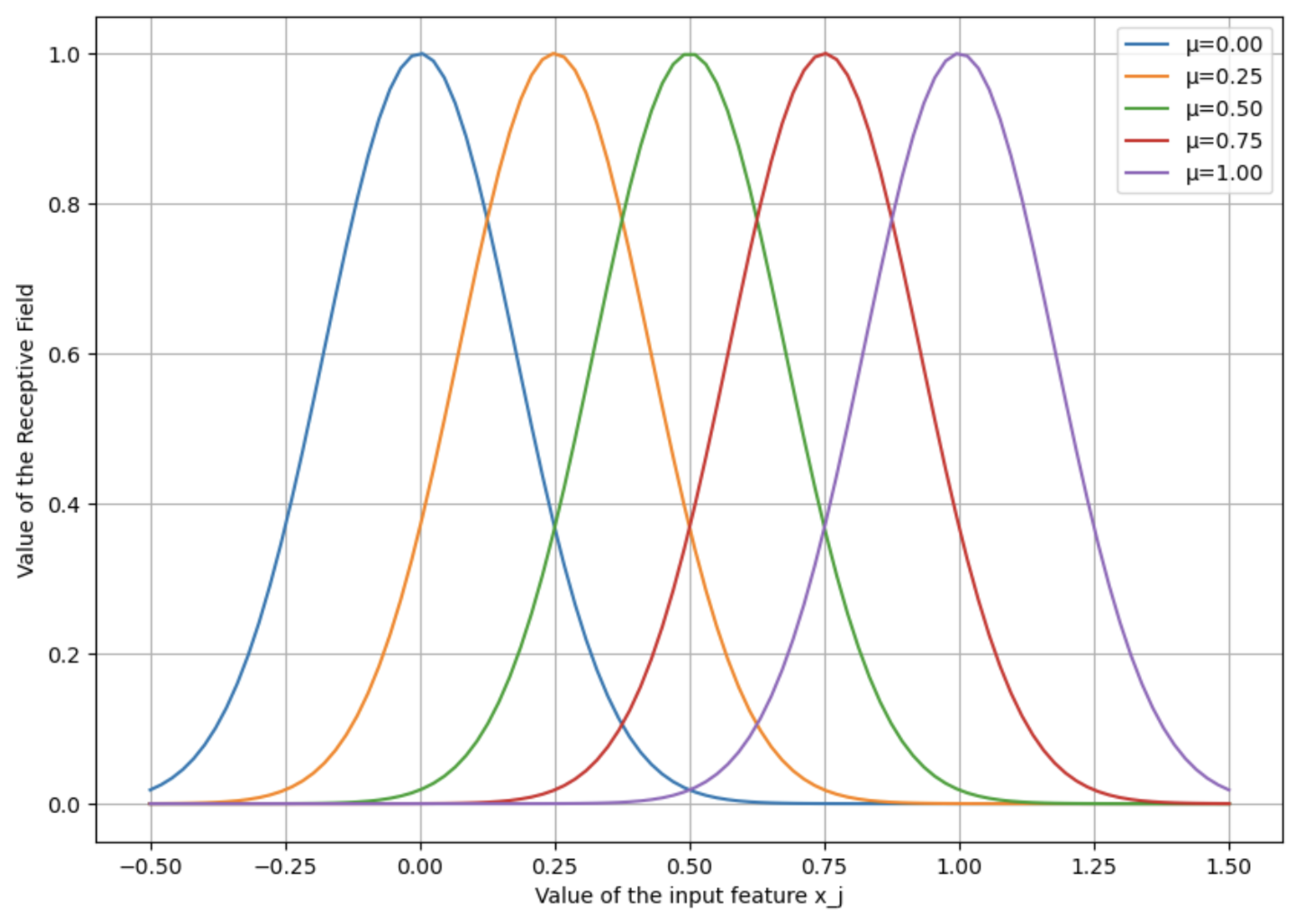
- Gaussian Receptive Fields (GRFs): This step was intended to increase the separability of the data by transforming it into a space of higher dimension. At this stage, the range of each of the normalized feature vectors was divided into M equal intervals. At each interval , a Gaussian peak was constructed with a center and standard deviation (see Equation (1), Figure 2). The value of each component of the input vector was replaced by a set of values , which characterized the proximity of to the center of the j-th receptive field. Thus, the dimension of the input vector increased by the factor of M.
- (4)
- Spike encoding: To convert the normalized and GRF-processed input vectors into spike sequences, we used a frequency-based approach. With this encoding method, each input neuron (spike generator) emits spikes at a frequency during the entire sample time , where . Here, is the maximum frequency of spike emission and k is the value of the input vector component. After time has passed, the generators do not emit spikes for ms to allow for the neuron potentials to return to their original values.

Figure 2.
An example of Gaussian receptive fields with the number of fields being equal to 5. The input feature was intersected with overlapping Gaussian fields to produce a vectorized feature representation: .
Figure 2.
An example of Gaussian receptive fields with the number of fields being equal to 5. The input feature was intersected with overlapping Gaussian fields to produce a vectorized feature representation: .
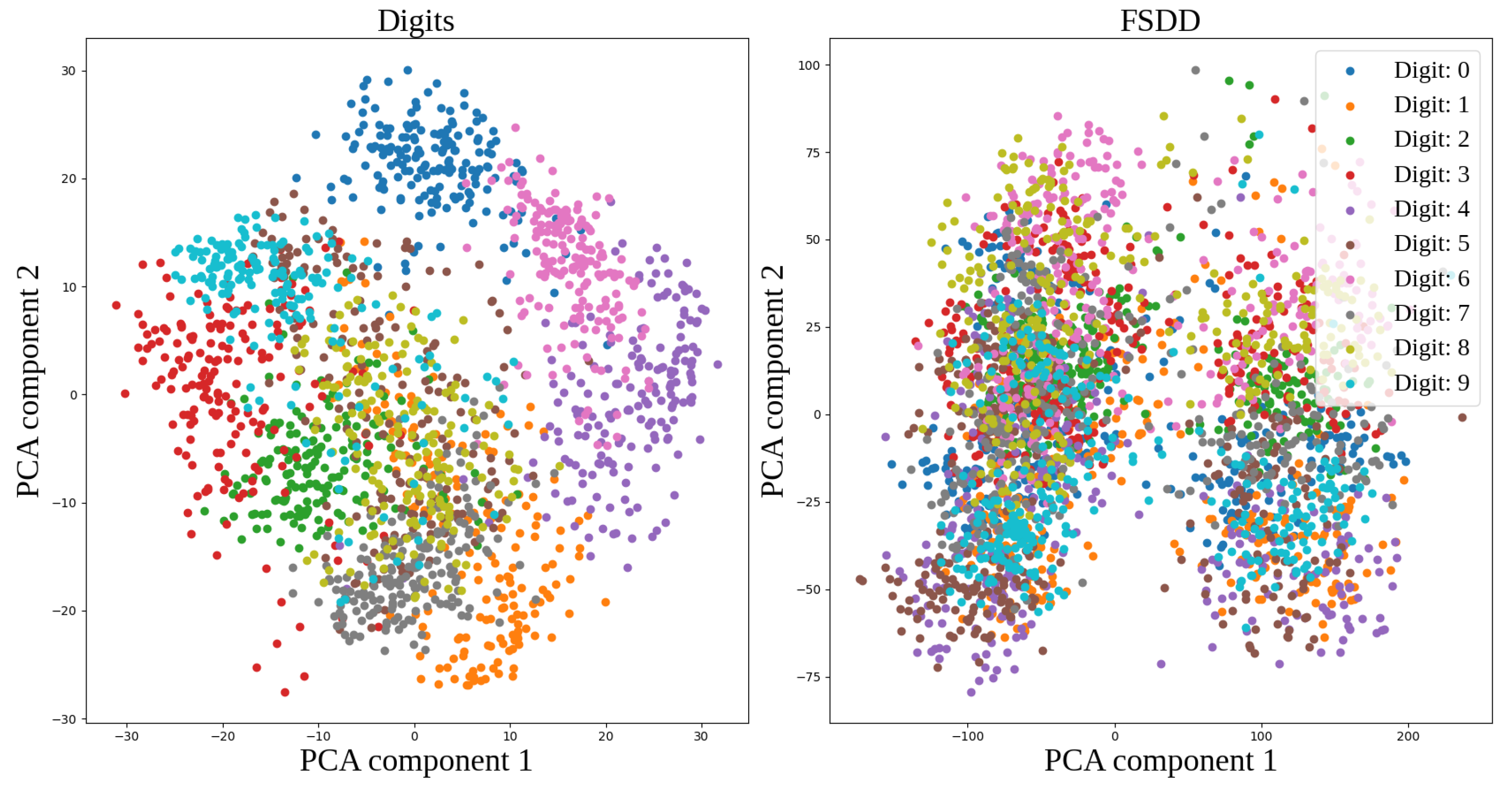
To illustrate the relative complexity of both datasets, we performed dimensionality reduction using principal component analysis (PCA) on both datasets after the feature engineering stage. This method allows us to reduce the feature space to two dimensions and visually assess the degree of nonlinear separability of the samples. Its results are shown in Figure 3.
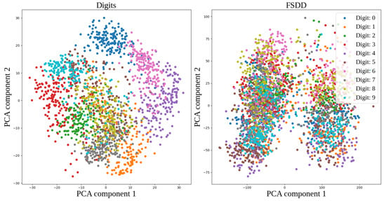
Figure 3.
Principal component analysis for the Digits and FSDD datasets.
It can be clearly seen that the classification boundaries for the MFCC-encoded FSDD dataset have to be much more complex in order to achieve high accuracy. In other words, in this work, the handwritten digits dataset acts as a weak baseline, and it was used to assess the general capability of the sparsity methods under consideration, while the spoken digits dataset played the role of a more challenging benchmark.
3.2. Synaptic Plasticity Models
In this work, we considered two memristive plasticity models: nanocomposite (NC) [28] and poly-p-xylylene (PPX) [29]. These models were proposed to approximate the real-world dependence of synaptic conductance change on the value of the conductance w and on the time difference between presynaptic and postsynaptic spikes, and they are defined in Equations (2) and (3).
In Equation (2), , , ms, ms, ms, ms.
Here, ms, , , , , , , , and .
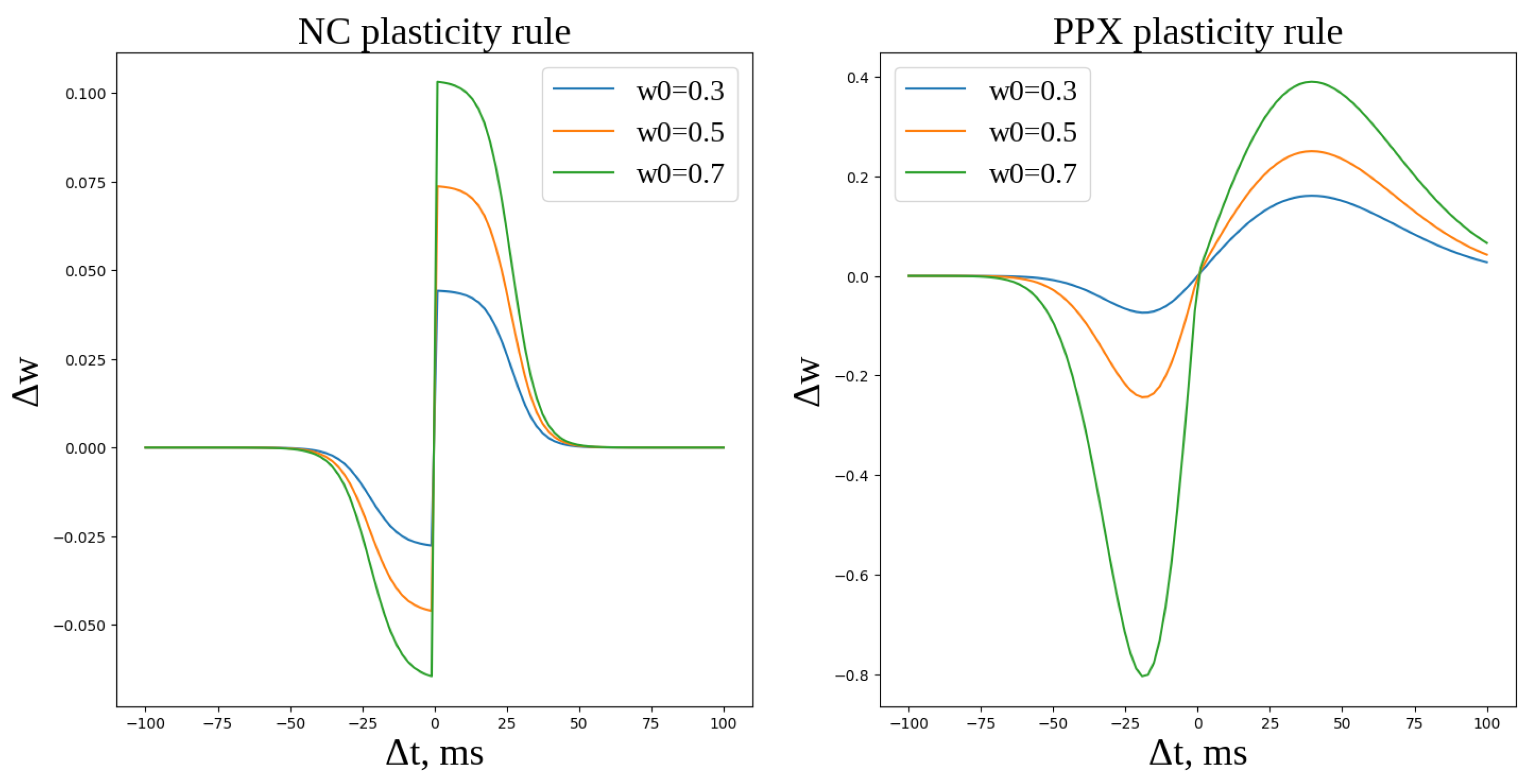
Both memristive plasticity rules are shown in Figure 4. It can be seen that the models differ both in their dependence on the initial weight and in their spread along the axis: NC plasticity is localized within the ms range and is relatively symmetric, while the PPX plasticity covers a much larger range and exhibits asymmetric behavior depending on the initial weight and the sign of . Due to these differences, the training process differed for both rules, thus facilitating a broader study of the capabilities and limitations of the proposed methods.
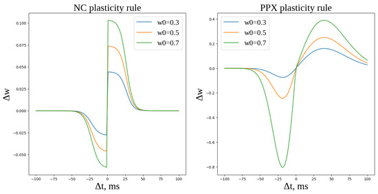
Figure 4.
NC and PPX memristive plasticity curves for different values of the initial weight .
Additionally, we considered a classical additive spike timing-dependent plasticity (STDP) [30] model to study the impact of sparcity on the memristor-based network in relation to the simpler synapse models.
3.3. Spiking Classification Models
Within the framework of the frequency approach to encoding input data, we considered a hybrid architecture consisting of a three-layer Winner Takes All (WTA) network [21], and this serves as a feature extraction module in combination with a formal classifier.
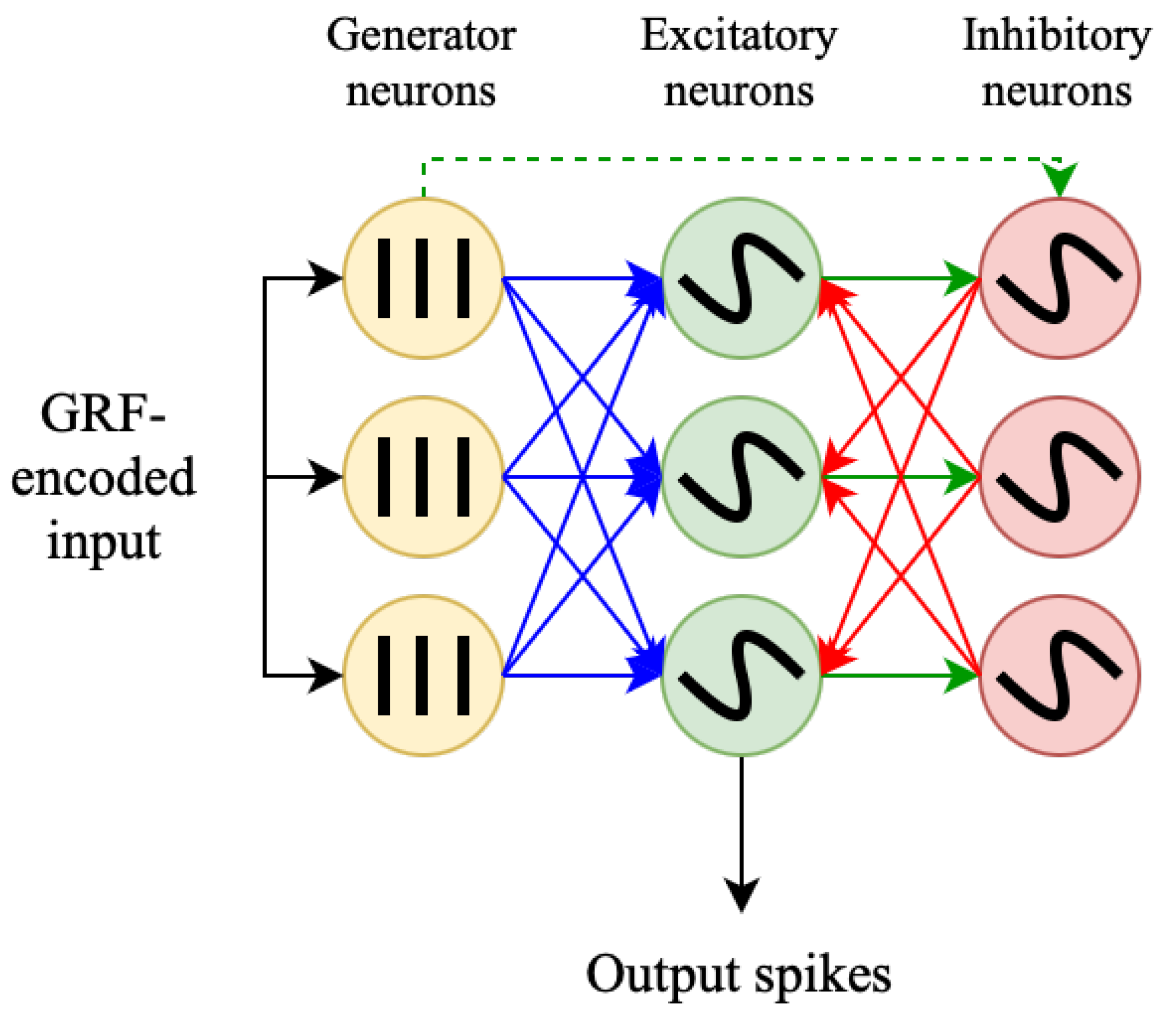
The WTA network is based on three layers (see Figure 5). The input layer consists of spike generators that convert input vectors into spike sequences according to the algorithm described above. The size of the input layer corresponds to the size of the input vector after preprocessing steps. The generated spike sequences are transmitted to the layer of leaky integrate-and-fire (LIF) neurons with an adaptive threshold (excitatory layer). This layer is connected to the input via trainable weights with one of the previously described plasticities according to the “all-to-all” rule. The number of neurons in the excitatory layer can be optimized depending on the complexity of the problem being solved. In turn, the excitatory layer is connected to the third layer of non-adaptive LIF neurons of the same size, which is called the inhibitory layer. Connections from the excitatory to the inhibitory layer are not trainable and have a fixed positive weight . In this case, each neuron in the excitatory layer is connected to a single neuron (partner) in the inhibitory layer. The connections directed from the inhibitory layer to the excitatory layer are called inhibitory connections. These connections are static and have a weight . Each neuron in the inhibitory layer is connected to all neurons in the excitatory layer except to its partner. Finally, the generators in the input layer are also connected to inhibitory neurons by randomly distributed static links with a weight . In all our experiments, the number of such connections was equal to 10% of the number of connections between the input and excitatory layers.
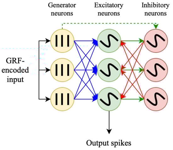
Figure 5.
WTA spiking neural network topology. Poisson generators, adaptive excitatory LIF neurons, and inhibitory LIF neurons are shown in yellow, green, and red, respectively. Trainable synapses are depicted in blue, excitatory-to-inhibitory connections are shown in green, and inhibitory-to-excitatory connections are denoted in red. Finally, generator-to-inhibitory connections are expressed using a dashed green arrow.
The spiking neural network was implemented using the NEST simulator [31].
We chose logistic regression (LGR), which was optimized for multi-class problems, and we used the one-versus-all (OVR) scheme as the formal classifier [32].
In this work, we considered two methods for reducing the connectivity in the WTA network: an ensemble of several classifiers trained using the bagging technique and sparse connectivity between layers.
3.3.1. Classification Ensemble
The bagging method was chosen as an ensemble creation technique; several identical classifiers were trained on subsets of input data, after which their predictions were then aggregated by voting. This method has several advantages compared to using a single larger network; in particular, it reduces the total number of connections within the network and increases the classification speed due to parallelization. In addition, it allows you to break unwanted correlations in the training dataset, thus resulting in improved architecture stability.
Connectivity within an ensemble is controlled using the following parameters:
- –
- : Defines the number of models within the ensemble.
- –
- max_features: Determines the proportion of input features that are passed to the input of each of the models in the ensemble.
In addition, the bagging architecture allows one to regulate the number of examples on which each network is trained using the max_samples parameter.
The ensemble was implemented using the BaggingClassifier method of the Scikit-Learn [25] library. In all experiments, which were based on the preliminary empirical observations, the parameters and were fixed.
3.3.2. Sparse Connectivity
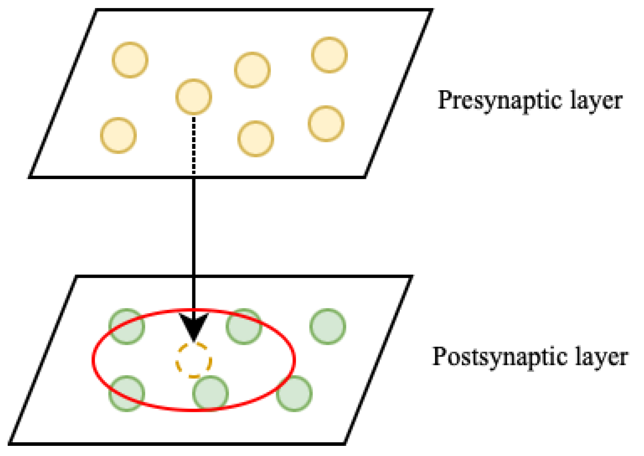
Another way through which to reduce the connectivity of a spike network is to set a rule that allows you to regulate the number of connections and their organization. To this end, we formally placed the neurons of the excitatory and inhibitory layers on two-dimensional square grids of a 1 mm × 1 mm size (the dimension was chosen for the convenience of further presentation), and these were oriented mirror-image relative to each other. The neurons on the grids may be arranged irregularly. The initialization of sparse connections occurred according to the following algorithm:
- (1)
- The presynaptic neuron projects onto the plane of the postsynaptic neurons.
- (2)
- The projection of the presynaptic neuron becomes the center of a circular neighborhood, and all postsynaptic neurons within which will be connected to this presynaptic neuron with some probability.
This process is shown schematically in Figure 6.

Figure 6.
Sparse connectivity: neuron projection. The projection neighborhood is shown in red; all postsynaptic neurons inside it will be connected to the projected presynaptic neuron.
Thus, connectivity within the network is regulated using two parameters:
- –
- Probability P of connection formation between pre- and post-synaptic neurons.
- –
- The radius of the circular neighborhood is R. This parameter is defined only for connections between the inhibitory and excitatory layers since neurons in the input layer do not have a spatial structure.
Both methods, as well as their combination, are expressed in a generalized form in Algorithm 1. This algorithm can be used for both proposed methods, as well as their combination, since the behavior of the network is determined by the parameters , , , and . In the case of a sparse WTA network, an ensemble consists of one network (); furthermore, in the case of a bagging ensemble of fully-connected WTA networks, randomized sparse connectivity is not applied (). A combined approach, therefore, requires specifying all four parameters. The generalized decoding procedure using a logistic regression approach is detailed in Algorithm 2.
| Algorithm 1 SNN learning process |
| Input: training data matrix with dimensions of the preprocessed input vectors of each sample in the dataset, neuron parameters, plasticity parameters, and synapse parameters Training parameters . Sparsity parameters: , max_features, max_samples, , , , and Network parameters: Table 1 Output data An ensemble containing spiking neural networks, which are vectors of neuron activity frequencies in the excitatory layer for each example of the training set .
|
| Algorithm 2 SNN decoding process |
Input: a collection F containing output frequencies of the excitatory layers of SNNs in the ensemble corresponding to each sample in the dataset, where each element contains frequency vectors obtained from the SNNs in the ensemble. Output data: a vector C of predicted class labels for each sample in the dataset.
|

Table 1.
Experimental settings for the WTA network.
Table 1.
Experimental settings for the WTA network.
| Digits | FSDD | ||||||
|---|---|---|---|---|---|---|---|
| Reduction Type | Parameter | STDP | NC | PPX | STDP | NC | PPX |
| Base | norm | L2 | STD | STD | L2 | STD | L2 |
| 5 | 5 | 5 | 10 | 10 | 10 | ||
| 550 | 550 | 550 | 550 | 550 | 550 | ||
| 1 | 1 | 1 | 1 | 1 | 1 | ||
| 130 | 130 | 130 | 130 | 130 | 130 | ||
| 30 | 30 | 30 | 30 | 30 | 30 | ||
| frequency | 600 | 350 | 450 | 800 | 800 | 800 | |
| 5 | 4 | 6 | 5 | 4 | 4 | ||
| 3 | 3 | 3 | 3 | 3 | 3 | ||
| 18 | 20 | 20 | 20 | 20 | 20 | ||
| −13 | −15 | −15 | −13 | −15 | −13 | ||
| Sparse Conn. | 0.4 | 0.4 | 0.4 | 0.4 | 0.4 | 0.4 | |
| 0.4 | 0.4 | 0.4 | 0.4 | 0.4 | 0.4 | ||
| 0.9 | 0.9 | 0.9 | 0.9 | 0.9 | 0.9 | ||
| Bagging | 50 | 50 | 50 | 50 | 50 | 50 | |
| 11 | 11 | 11 | 11 | 11 | 11 | ||
| Bagging + Sparse | 50 | 50 | 50 | 50 | 50 | 50 | |
| 11 | 11 | 11 | 11 | 11 | 11 | ||
| 0.7 | 0.7 | 0.7 | 0.7 | 0.7 | 0.7 | ||
| 0.7 | 0.7 | 0.7 | 0.7 | 0.7 | 0.7 | ||
| 0.9 | 0.9 | 0.9 | 0.9 | 0.9 | 0.9 | ||
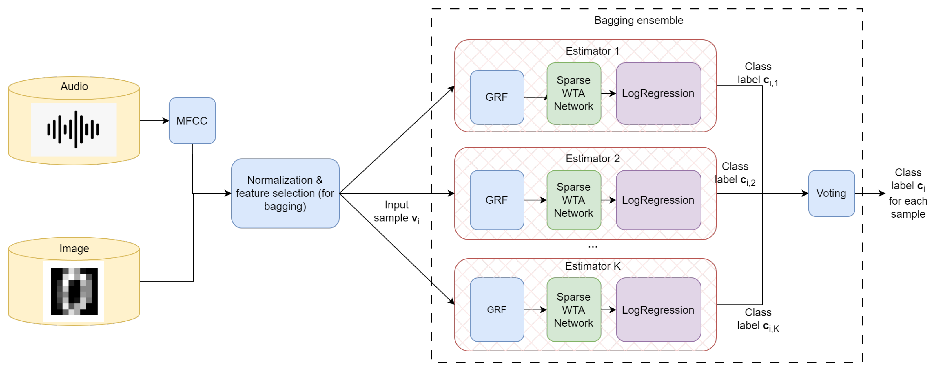
The classification process is additionally visualized in Figure 7. Depending on the experimental settings, the number of the models in the ensemble may be equal to one (base WTA and sparse WTA), and the weight initialization may be performed in accordance with the sparse connectivity approach or in a fully connected manner.

Figure 7.
The testing pipeline for the proposed approach. It is depicted for both audio and image data: the former requires MFCC preprocessing, while the latter does not. After preprocessing, the resulting feature vectors were normalized and analyzed by each model in the ensemble.The predictions of multiple estimators were aggregated via voting, thus producing the final class label.
4. Experiments and Results
Experiments on the Digits dataset were conducted using hold-out cross-validation; then, 20% of the training examples were used for testing. On FSDD, a fixed testing dataset was used. For all experiments, such parameters as the number of neurons in the networks, the number of receptive fields, and the number of networks in the ensemble were selected for each plasticity and for each dataset by maximizing the training classification accuracy. The selection was performed automatically using the tree-parzen estimator (TPE) algorithm implemented in HyperOpt [33] (an open-source Python package). For all of the three methods under consideration, the parameters across plasticity models and datasets were fixed, thus ensuring a fair comparison. The source code of all the connectivity reduction methods is available in our repository (see Funding information below).
In Table 1, we present the hyperparameters of SNN that were used for each of the considered datasets and plasticity models:
- –
- norm—the input normalization method: L2 or standard scaling (STD);
- –
- —the number of Gaussian receptive fields (GRFs);
- –
- —the number of excitatory neurons in the network;
- –
- —the number of networks in the bagging ensemble (for the ensemble approach specifically, everywhere else it is equal to 1);
- –
- and —the characteristic time of the membrane potential decay for the excitatory and inhibitory neurons in milliseconds;
- –
- frequency—the maximal spiking frequency of the Poisson generators;
- –
- and —the refractory time for the excitatory and inhibitory neurons in milliseconds;
- –
- and —the synaptic weights of the excitatory-to-inhibitory and inhibitory-to-excitatory connections, respectively;
- –
- —the probability of forming a connection between an input and an excitatory neuron in the sparse WTA network;
- –
- —the probability of forming a connection between an inhibitory and an excitatory neuron in the sparse WTA network;
- –
- —the projection radius for inhibitory-to-excitatory connections in the sparse WTA network.
In all experiments, the time for submitting one example to the WTA network was 350 ms, which was followed by a relaxation period of 50 ms, thereby resulting in a processing time of ms per sample, where learning took place over one epoch. As a baseline, we conducted an experiment using the classical WTA network (see Section 3.3).
Additionally, we presented the number of connections within the network with a breakdown by type of the pre- and postsynaptic neurons. Table 2 demonstrates the connectivity within the base WTA network. The connections for the base network and the bagging ensemble were calculated, as shown in Equation (4). In the equations, is equal to the number of input features, denotes the number of excitatory neurons, is a fraction of the inhibitory neurons connected to the generator layer, is the number of estimators within the ensemble, and is for the base WTA network. For the sparse WTA network, the connections were counted manually from the weight checkpoints due to their stochastic nature.
Table 2.
Connectivity within the base WTA network.
Here, is equal to the number of input features, denotes the number of excitatory neurons, is a fraction of the inhibitory neurons connected to the generator layer, is the number of estimators within the ensemble, and is for the base WTA network. For the sparse WTA network, the connections were counted manually from the weight checkpoints due to their stochastic nature.
After applying the considered methods for reducing the number of connections in the WTA network, the connectivity of the resulting models was obtained, as presented in Table 3.
Table 3.
Connectivity within the sparse WTA network.
The experimental results for applying different types of reduction methods are presented in Table 4, and they are also expressed using the F1-score metric, which is defined in Equation (5).
Table 4.
Experimental results for the WTA network. The maximum F1-scores for each experiment are highlighted in bold.
The obtained accuracies are consistent with and superior to the results reported in our previous works on spiking neural networks with memristive plasticity and without sparse connectivity:
- Digits
- 0.83–0.86 F1 from the article [23]. The best performance was obtained by a one-layer SNN with 1600 neurons and 2,660,800 connections (vs. the bagging WTA SNN model with 550 neurons and 221,000 connections)
- FSDD
- 0.81–0.93 F1 from the article [34], where the best scores were achieved by WTA SNN with 400 neurons and 243,600 connections. For comparison, the proposed sparse bagging WTA SNN model containing 550 neurons and 151,217 connections achieved the same performance (F1: 0.93).
It also follows from Table 5 that the resulting SNN models with sparse connectivity and memristive plasticity demonstrated high accuracy compared to the other algorithms, including non-spiking ones.
Table 5.
Comparison of results for both of the classification tasks. * indicates the accuracy metric. The maximum performance scores for our experiments and literature sources are highlighted in bold.
5. Discussion
To evaluate the effectiveness of the connectivity reduction methods, we introduced the connectivity index , as defined in Equation (6):
Here, and are the total number of connections in the sparse network and the equivalent fully connected WTA network, respectively. Based on this definition, the efficiency of the connectivity reduction method can be assessed by calculating the ratio of the classification accuracy to the connectivity index (see Equation (7), where the efficiency is represented by the index ).
The values of the connectivity and efficiency indices for different datasets, plasticities, and network types are presented in Table 6. The motivation for the proposed indices lies in assessing the accuracy-per-connection ratio, which is a more robust comparison metric for the proposed methods compared to raw accuracy.
Table 6.
Efficiency estimation of the different sparsity types. The best values are marked in bold.
From the table above, it follows that, in our experiments, the relative efficiency of spike networks with sparse connectivity in comparison to ensembles of spike networks was found to be slightly higher; on average, across plasticities and datasets, the efficiency of the sparsely connected WTA network was 2.2, while the efficiency of bagging was, on average, equal to 2.1. However, due to the small scale of this difference, we concluded that both methods can be effectively used to reduce connectivity depending on the specifics of the problem and the hardware requirements. If the experimental setting facilitates only the reduction in static connections and supports ensembles, bagging is a preferable option, while sparse connectivity may be used in situations where only a single larger network is feasible.
The combination of these two methods yielded the highest efficiency of 2.8, on average, with an average connectivity index equal to 0.32. Therefore, if combining both approaches is possible for a given problem, the resulting accuracy-per-connection efficiency will be the highest.
6. Conclusions
In this work, we compared two approaches to connectivity reduction in memristive spiking neural networks: the bagging ensemble technique and probabilistic sparse connectivity. Using a three-layer WTA network, we demonstrated that both methods achieved competitive performance on the handwritten digits and spoken digits classification tasks, with a combination of both approaches achieving the highest efficiency. On the Digits dataset, the bagging ensemble yielded an F1-score of 0.95, 0.94, and 0.94 for the STDP, NC, and PPX plasticity rules, respectively, while the sparse WTA network achieved 0.94, 0.93, and 0.94, respectively; furthermore, a combined Bagging + Sparse model, in turn, yielded F1-scores of 0.87, 0.93, and 0.94, respectively. On FSDD, the F1-score values lay within the 0.89–0.93 range for the ensemble of WTA networks, within the 0.84–0.92 interval for the sparse WTA network, and within the 0.88–0.91 range for the combined model. The resulting models were found to be superior in accuracy to well-known spiking neural network solutions, and they also corresponded to the level of other non-spike algorithms. Additionally, by studying the ratio between the proposed connectivity index and the F1-score, we showed that the bagging ensemble and the sparse WTA network achieved an almost equal efficiency, while the combination of both methods yielded a 20% higher average efficiency coefficient value.
Thus, the created combination of methods can be used as a computational technology for creating spike neural network models for implementation on neurochips in inference mode. Also, the developed architectures of spiking neural networks can be used for the subsequent implementation of online learning on neuromorphic chips with memristive connections. In our future research, we plan to expand the scope of the classification problems for image and audio data that can be solved using the proposed methods (e.g., the CIFAR-10, Google Speech Commands dataset, etc.), as well as work on hardware implementations of the designed networks.
Author Contributions
Conceptualization, R.R., Y.D. and D.V.; methodology, R.R., Y.D. and D.V.; software, Y.D., D.V. and A.S.(Alexey Serenko); validation, Y.D. and D.V.; formal analysis, A.S. (Alexander Sboev) and V.I.; investigation, R.R., A.S. (Alexander Sboev) and V.I.; resources, R.R.; data curation, A.S. (Alexey Serenko); writing—original draft preparation, Y.D.; writing—review and editing, R.R. and A.S. (Alexey Serenko); visualization, Y.D.; supervision, R.R.; project administration, R.R.; funding acquisition, R.R. All authors have read and agreed to the published version of the manuscript.
Funding
The study was supported by a grant from the Russian Science Foundation №21-11-00328, https://rscf.ru/project/21-11-00328/ (accessed 8 February 2024). The bagging ensemble and sparse connectivity model preparation code is available at https://github.com/sag111/Sparse-WTA-SNN (accessed 8 February 2024).
Data Availability Statement
The Digits dataset is publicly available through the Scikit-Learn Python library: https://scikit-learn.org/stable/ (accessed 8 February 2024). The FSDD dataset can be freely obtained from https://github.com/Jakobovski/free-spoken-digit-dataset (accessed 8 February 2024).
Acknowledgments
Computational experiments were carried out using the equipment of the Center for Collective Use “Complex for Modeling and Processing Data of Mega-Class Research Installations” of the National Research Center “Kurchatov Institute”, http://ckp.nrcki.ru/ (accessed 8 February 2024).
Conflicts of Interest
The authors declare no conflicts of interest. The funding agencies had no role in the design of the study; in the collection, analyses, or interpretation of data; or in the writing of the manuscript.
Abbreviations
The following abbreviations are used in this manuscript:
| SNN | Spiking neuralnNetwork |
| ANN | Artificial neural network |
| STDP | Spike timing-dependent plasticity |
| NC | Nanocomposite |
| PPX | Poly-p-xylylene |
| WTA | Winner Takes All |
| FSDD | Free Spoken Digits Dataset |
References
- Merolla, P.A.; Arthur, J.V.; Alvarez-Icaza, R.; Cassidy, A.S.; Sawada, J.; Akopyan, F.; Jackson, B.L.; Imam, N.; Guo, C.; Nakamura, Y.; et al. A million spiking-neuron integrated circuit with a scalable communication network and interface. Science 2014, 345, 668–673. [Google Scholar] [CrossRef]
- Davies, M.; Srinivasa, N.; Lin, T.H.; Chinya, G.; Cao, Y.; Choday, S.H.; Dimou, G.; Joshi, P.; Imam, N.; Jain, S.; et al. Loihi: A neuromorphic manycore processor with on-chip learning. IEEE Micro 2018, 38, 82–99. [Google Scholar] [CrossRef]
- Rajendran, B.; Sebastian, A.; Schmuker, M.; Srinivasa, N.; Eleftheriou, E. Low-Power Neuromorphic Hardware for Signal Processing Applications: A review of architectural and system-level design approaches. IEEE Signal Process. Mag. 2019, 36, 97–110. [Google Scholar] [CrossRef]
- Ambrogio, S.; Narayanan, P.; Okazaki, A.; Fasoli, A.; Mackin, C.; Hosokawa, K.; Nomura, A.; Yasuda, T.; Chen, A.; Friz, A.; et al. An analog-AI chip for energy-efficient speech recognition and transcription. Nature 2023, 620, 768–775. [Google Scholar] [CrossRef] [PubMed]
- Shvetsov, B.S.; Minnekhanov, A.A.; Emelyanov, A.V.; Ilyasov, A.I.; Grishchenko, Y.V.; Zanaveskin, M.L.; Nesmelov, A.A.; Streltsov, D.R.; Patsaev, T.D.; Vasiliev, A.L.; et al. Parylene-based memristive crossbar structures with multilevel resistive switching for neuromorphic computing. Nanotechnology 2022, 33, 255201. [Google Scholar] [CrossRef] [PubMed]
- Matsukatova, A.N.; Iliasov, A.I.; Nikiruy, K.E.; Kukueva, E.V.; Vasiliev, A.L.; Goncharov, B.V.; Sitnikov, A.V.; Zanaveskin, M.L.; Bugaev, A.S.; Demin, V.A.; et al. Convolutional Neural Network Based on Crossbar Arrays of (Co-Fe-B) x (LiNbO3) 100- x Nanocomposite Memristors. Nanomaterials 2022, 12, 3455. [Google Scholar] [CrossRef] [PubMed]
- Amiri, M.; Jafari, A.H.; Makkiabadi, B.; Nazari, S. Recognizing intertwined patterns using a network of spiking pattern recognition platforms. Sci. Rep. 2022, 12, 19436. [Google Scholar] [CrossRef]
- Cohen, G.; Afshar, S.; Tapson, J.; Van Schaik, A. EMNIST: Extending MNIST to handwritten letters. In Proceedings of the 2017 International Joint Conference on Neural Networks (IJCNN), Anchorage, AK, USA, 14–19 May 2017; pp. 2921–2926. [Google Scholar]
- Georghiades, A.; Belhumeur, P.; Kriegman, D. From Few to Many: Illumination Cone Models for Face Recognition under Variable Lighting and Pose. IEEE Trans. Pattern Anal. Mach. Intell. 2001, 23, 643–660. [Google Scholar] [CrossRef]
- Samaria, F.; Harter, A. Parameterisation of a stochastic model for human face identification. In Proceedings of the 1994 IEEE Workshop on Applications of Computer Vision, Sarasota, FL, USA, 5–7 December 1994; pp. 138–142. [Google Scholar] [CrossRef]
- Emery, R.; Yakovlev, A.; Chester, G. Connection-centric network for spiking neural networks. In Proceedings of the 2009 3rd ACM/IEEE International Symposium on Networks-on-Chip, La Jolla, CA, USA, 10–13 May 2009; pp. 144–152. [Google Scholar]
- Saunders, D.J.; Patel, D.; Hazan, H.; Siegelmann, H.T.; Kozma, R. Locally connected spiking neural networks for unsupervised feature learning. Neural Netw. 2019, 119, 332–340. [Google Scholar] [CrossRef]
- Chen, Y.; Yu, Z.; Fang, W.; Huang, T.; Tian, Y. Pruning of deep spiking neural networks through gradient rewiring. arXiv 2021, arXiv:2105.04916. [Google Scholar]
- Nguyen, T.N.; Veeravalli, B.; Fong, X. Connection pruning for deep spiking neural networks with on-chip learning. In Proceedings of the International Conference on Neuromorphic Systems 2021, Wuhan, China, 11–14 October 2021; pp. 1–8. [Google Scholar]
- Lien, H.H.; Chang, T.S. Sparse compressed spiking neural network accelerator for object detection. IEEE Trans. Circuits Syst. I Regul. Pap. 2022, 69, 2060–2069. [Google Scholar] [CrossRef]
- Tsai, C.C.; Yang, Y.H.; Lin, H.W.; Wu, B.X.; Chang, E.C.; Liu, H.Y.; Lai, J.S.; Chen, P.Y.; Lin, J.J.; Chang, J.S.; et al. The 2020 embedded deep learning object detection model compression competition for traffic in Asian countries. In Proceedings of the 2020 IEEE International Conference on Multimedia & Expo Workshops (ICMEW), London, UK, 6–10 July 2020; pp. 1–6. [Google Scholar]
- Han, B.; Zhao, F.; Zeng, Y.; Pan, W. Adaptive sparse structure development with pruning and regeneration for spiking neural networks. arXiv 2022, arXiv:2211.12219. [Google Scholar]
- Amir, A.; Taba, B.; Berg, D.; Melano, T.; McKinstry, J.; Di Nolfo, C.; Nayak, T.; Andreopoulos, A.; Garreau, G.; Mendoza, M.; et al. A low power, fully event-based gesture recognition system. In Proceedings of the IEEE Conference on Computer Vision and Pattern Recognition, Honolulu, HI, USA, 21–26 July 2017; pp. 7243–7252. [Google Scholar]
- Orchard, G.; Jayawant, A.; Cohen, G.K.; Thakor, N. Converting static image datasets to spiking neuromorphic datasets using saccades. Front. Neurosci. 2015, 9, 437. [Google Scholar] [CrossRef] [PubMed]
- Rathi, N.; Panda, P.; Roy, K. STDP-based pruning of connections and weight quantization in spiking neural networks for energy-efficient recognition. IEEE Trans. Comput.-Aided Des. Integr. Circuits Syst. 2018, 38, 668–677. [Google Scholar] [CrossRef]
- Diehl, P.U.; Cook, M. Unsupervised learning of digit recognition using Spike-Timing-Dependent Plasticity. Front. Comput. Neurosci. 2015, 9, 99. [Google Scholar] [CrossRef] [PubMed]
- Sboev, A.; Vlasov, D.; Rybka, R.; Davydov, Y.; Serenko, A.; Demin, V. Modeling the Dynamics of Spiking Networks with Memristor-Based STDP to Solve Classification Tasks. Mathematics 2021, 9, 3237. [Google Scholar] [CrossRef]
- Sboev, A.; Davydov, Y.; Rybka, R.; Vlasov, D.; Serenko, A. A Comparison of Two Variants of Memristive Plasticity for Solving the Classification Problem of Handwritten Digits Recognition. In Biologically Inspired Cognitive Architectures Meeting; Springer: Cham, Switzerland, 2021; pp. 438–446. [Google Scholar]
- Sboev, A.; Rybka, R.; Vlasov, D.; Serenko, A. Solving a classification task with temporal input encoding by a spiking neural network with memristor-type plasticity in the form of hyperbolic tangent. In AIP Conference Proceedings; AIP Publishing: Melville, NY, USA, 2023; Volume 2849. [Google Scholar]
- Pedregosa, F.; Varoquaux, G.; Gramfort, A.; Michel, V.; Thirion, B.; Grisel, O.; Blondel, M.; Prettenhofer, P.; Weiss, R.; Dubourg, V.; et al. Scikit-learn: Machine Learning in Python. J. Mach. Learn. Res. 2011, 12, 2825–2830. [Google Scholar]
- Jackson, Z.; Souza, C.; Flaks, J.; Pan, Y.; Nicolas, H.; Thite, A. Jakobovski/Free-Spoken-Digit-Dataset: V1.0.8, 2018. Available online: https://zenodo.org/records/1342401 (accessed on 20 February 2024).
- Aizawa, K.; Nakamura, Y.; Satoh, S. Advances in Multimedia Information Processing-PCM 2004: 5th Pacific Rim Conference on Multimedia, Tokyo, Japan, November 30–December 3, 2004, Proceedings, Part II; Springer: Berlin/Heidelberg, Germany, 2004; Volume 3332. [Google Scholar]
- Demin, V.; Nekhaev, D.; Surazhevsky, I.; Nikiruy, K.; Emelyanov, A.; Nikolaev, S.; Rylkov, V.; Kovalchuk, M. Necessary conditions for STDP-based pattern recognition learning in a memristive spiking neural network. Neural Netw. 2021, 134, 64–75. [Google Scholar] [CrossRef]
- Minnekhanov, A.A.; Shvetsov, B.S.; Martyshov, M.M.; Nikiruy, K.E.; Kukueva, E.V.; Presnyakov, M.Y.; Forsh, P.A.; Rylkov, V.V.; Erokhin, V.V.; Demin, V.A.; et al. On the resistive switching mechanism of parylene-based memristive devices. Org. Electron. 2019, 74, 89–95. [Google Scholar] [CrossRef]
- Song, S.; Miller, K.D.; Abbott, L.F. Competitive Hebbian learning through spike-timing-dependent synaptic plasticity. Nat. Neurosci. 2000, 3, 919–926. [Google Scholar] [CrossRef]
- Spreizer, S.; Mitchell, J.; Jordan, J.; Wybo, W.; Kurth, A.; Vennemo, S.B.; Pronold, J.; Trensch, G.; Benelhedi, M.A.; Terhorst, D.; et al. NEST 3.3. 2022. Available online: https://zenodo.org/records/6368024 (accessed on 20 February 2024).
- Buitinck, L.; Louppe, G.; Blondel, M.; Pedregosa, F.; Mueller, A.; Grisel, O.; Niculae, V.; Prettenhofer, P.; Gramfort, A.; Grobler, J.; et al. API design for machine learning software: Experiences from the scikit-learn project. In Proceedings of the ECML PKDD Workshop: Languages for Data Mining and Machine Learning, Prague, Czech Republic, 23–27 September 2013; pp. 108–122. [Google Scholar]
- Bergstra, J.; Yamins, D.; Cox, D.D. Hyperopt: A python library for optimizing the hyperparameters of machine learning algorithms. In Proceedings of the 12th Python in Science Conference, Austin, TX, USA, 24–29 June 2013; Citeseer: State College, PA, USA, 2013; Volume 13, p. 20. [Google Scholar]
- Vlasov, D.; Davydov, Y.; Serenko, A.; Rybka, R.; Sboev, A. Spoken digits classification based on Spiking neural networks with memristor-based STDP. In Proceedings of the 2022 International Conference on Computational Science and Computational Intelligence (CSCI), Las Vegas, NV, USA, 14–16 December 2022; pp. 330–335. [Google Scholar]
- Mitra, S.; Gilpin, L. The XAISuite framework and the implications of explanatory system dissonance. arXiv 2023, arXiv:2304.08499. [Google Scholar]
- Kashif, M.; Al-Kuwari, S. The impact of cost function globality and locality in hybrid quantum neural networks on NISQ devices. Mach. Learn. Sci. Technol. 2023, 4, 015004. [Google Scholar] [CrossRef]
- Kutikuppala, S. Decision Tree Learning Based Feature Selection and Evaluation for Image Classification. Int. J. Res. Appl. Sci. Eng. Technol. 2023, 11, 2668–2674. [Google Scholar] [CrossRef]
- Xu, H.; Kinfu, K.A.; LeVine, W.; Panda, S.; Dey, J.; Ainsworth, M.; Peng, Y.C.; Kusmanov, M.; Engert, F.; White, C.M.; et al. When are Deep Networks really better than Decision Forests at small sample sizes, and how? arXiv 2021, arXiv:2108.13637. [Google Scholar]
- Shougat, M.R.E.U.; Li, X.; Shao, S.; McGarvey, K.; Perkins, E. Hopf physical reservoir computer for reconfigurable sound recognition. Sci. Rep. 2023, 13, 8719. [Google Scholar] [CrossRef]
- Gemo, E.; Spiga, S.; Brivio, S. SHIP: A computational framework for simulating and validating novel technologies in hardware spiking neural networks. Front. Neurosci. 2024, 17, 1270090. [Google Scholar] [CrossRef]

Disclaimer/Publisher’s Note: The statements, opinions and data contained in all publications are solely those of the individual author(s) and contributor(s) and not of MDPI and/or the editor(s). MDPI and/or the editor(s) disclaim responsibility for any injury to people or property resulting from any ideas, methods, instructions or products referred to in the content. |
© 2024 by the authors. Licensee MDPI, Basel, Switzerland. This article is an open access article distributed under the terms and conditions of the Creative Commons Attribution (CC BY) license (https://creativecommons.org/licenses/by/4.0/).