Correlating the Plant Height of Wheat with Above-Ground Biomass and Crop Yield Using Drone Imagery and Crop Surface Model, A Case Study from Nepal

 ,
, 
 ,
, 
Abstract
:1. Introduction
- to understand how the easily measurable plant parameters such as plant height can be used to infer crop AGB, yield, and fertilizer optimization;
- to develop empirical regression models between the plant height and the AGB, and the plant height and the yield for wheat crops; and
- to validate empirical models for AGB and yield estimation with field measurements.
2. Materials and Methods
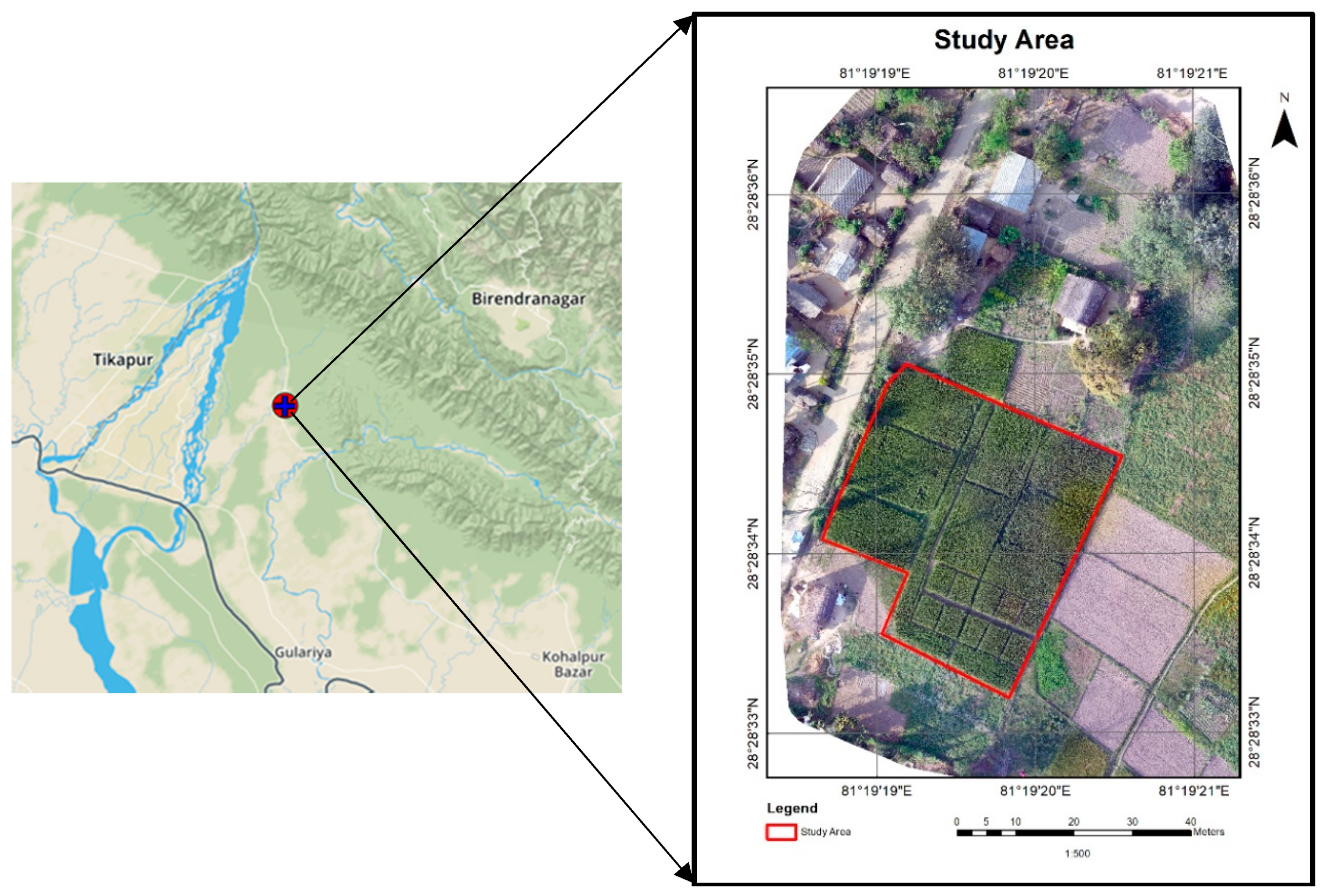
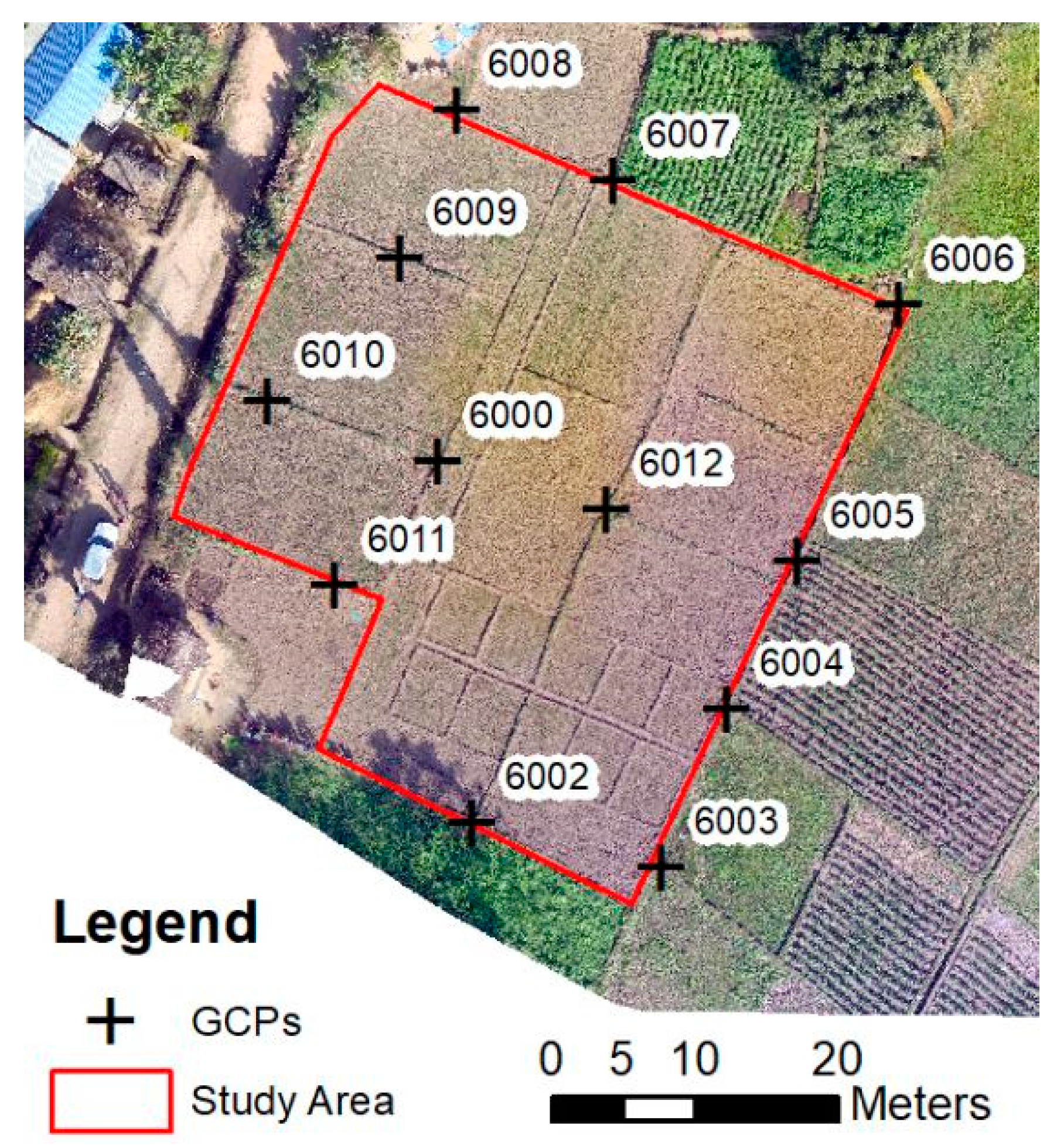
2.1. Study Area
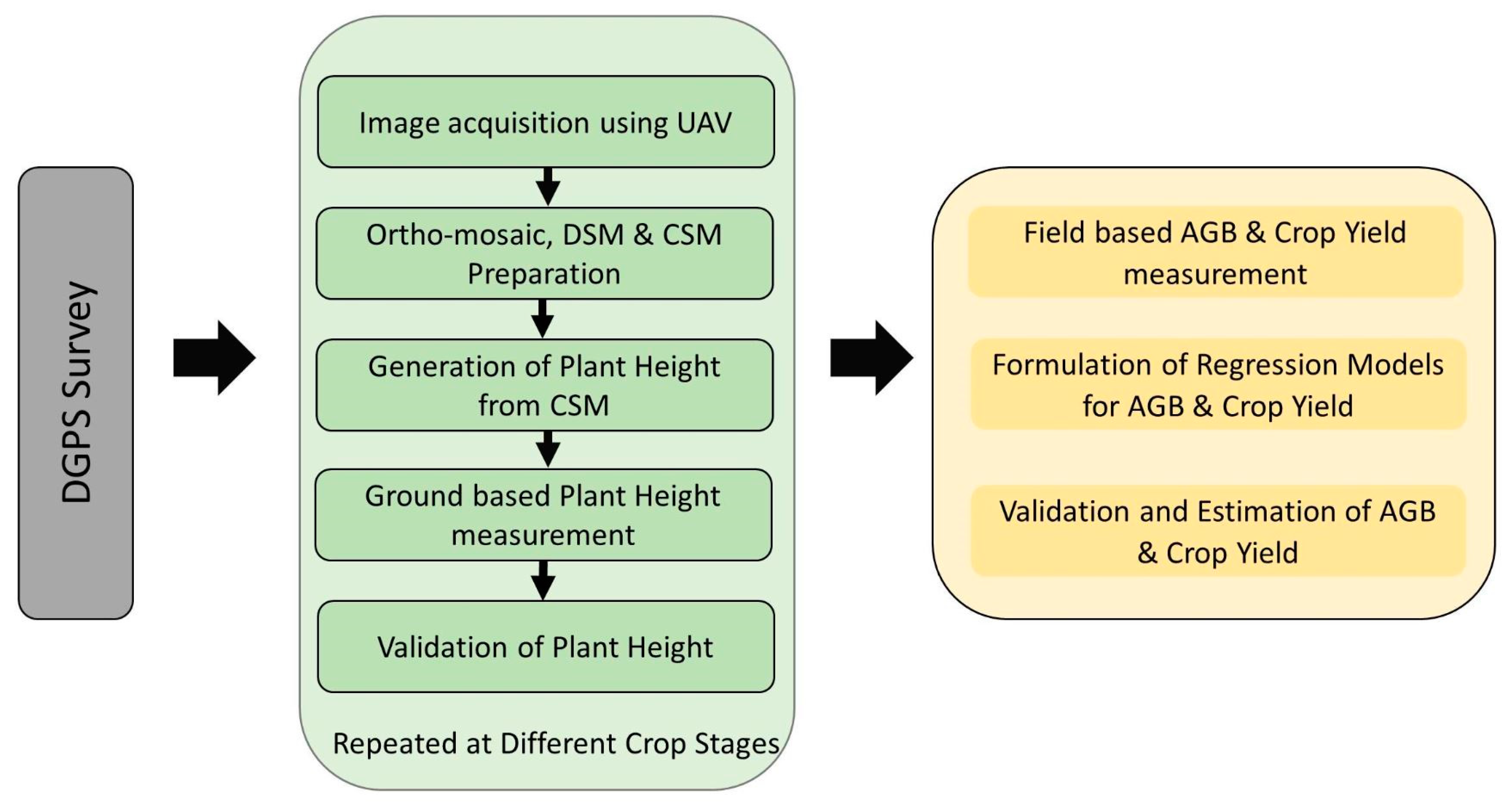
2.2. Methods
3. Results
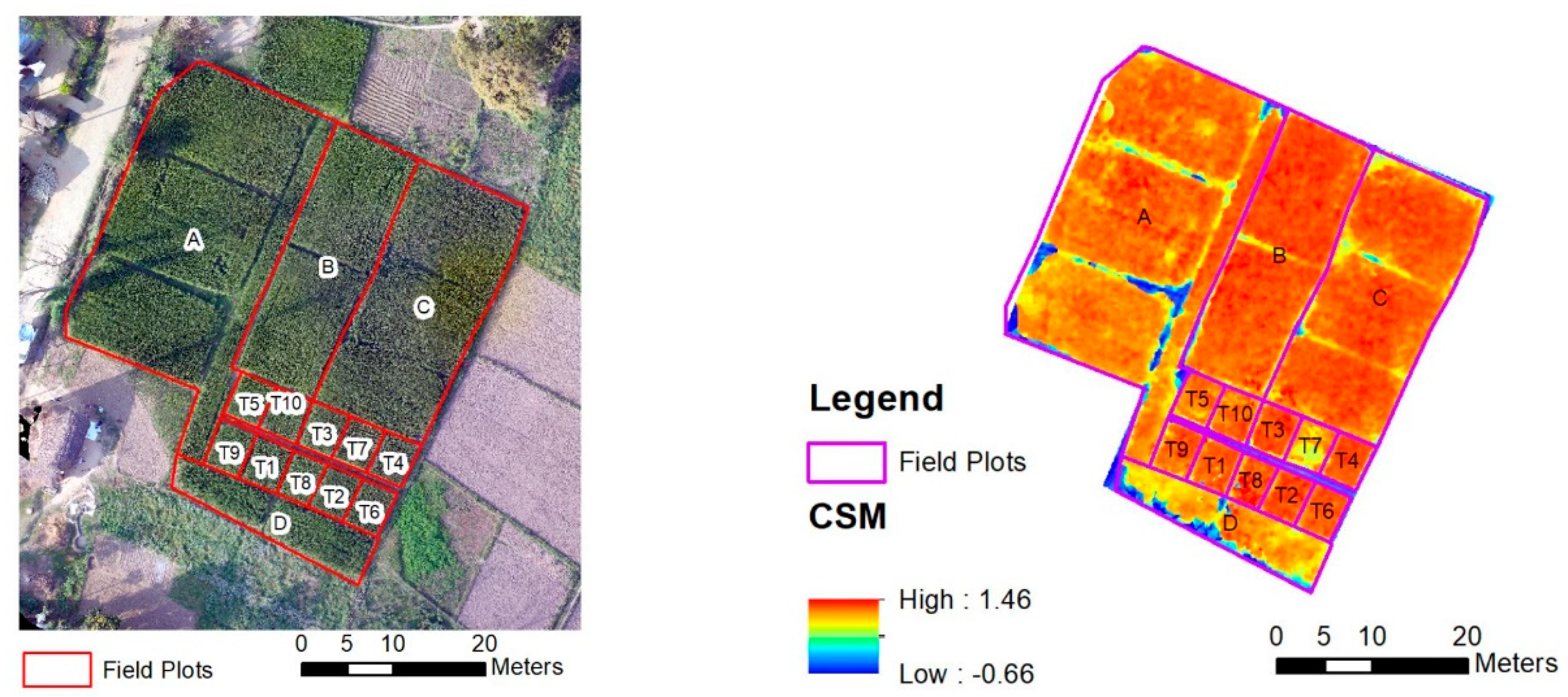
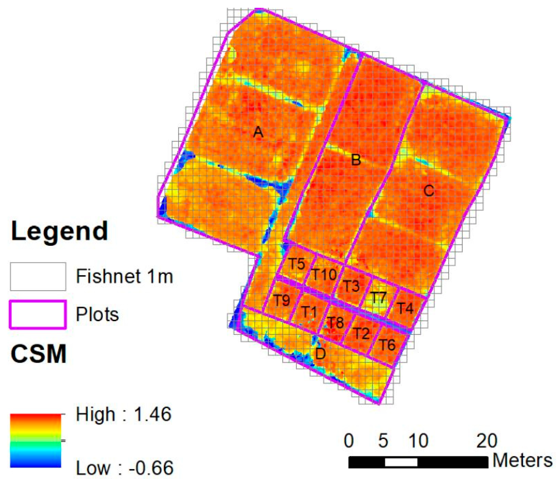
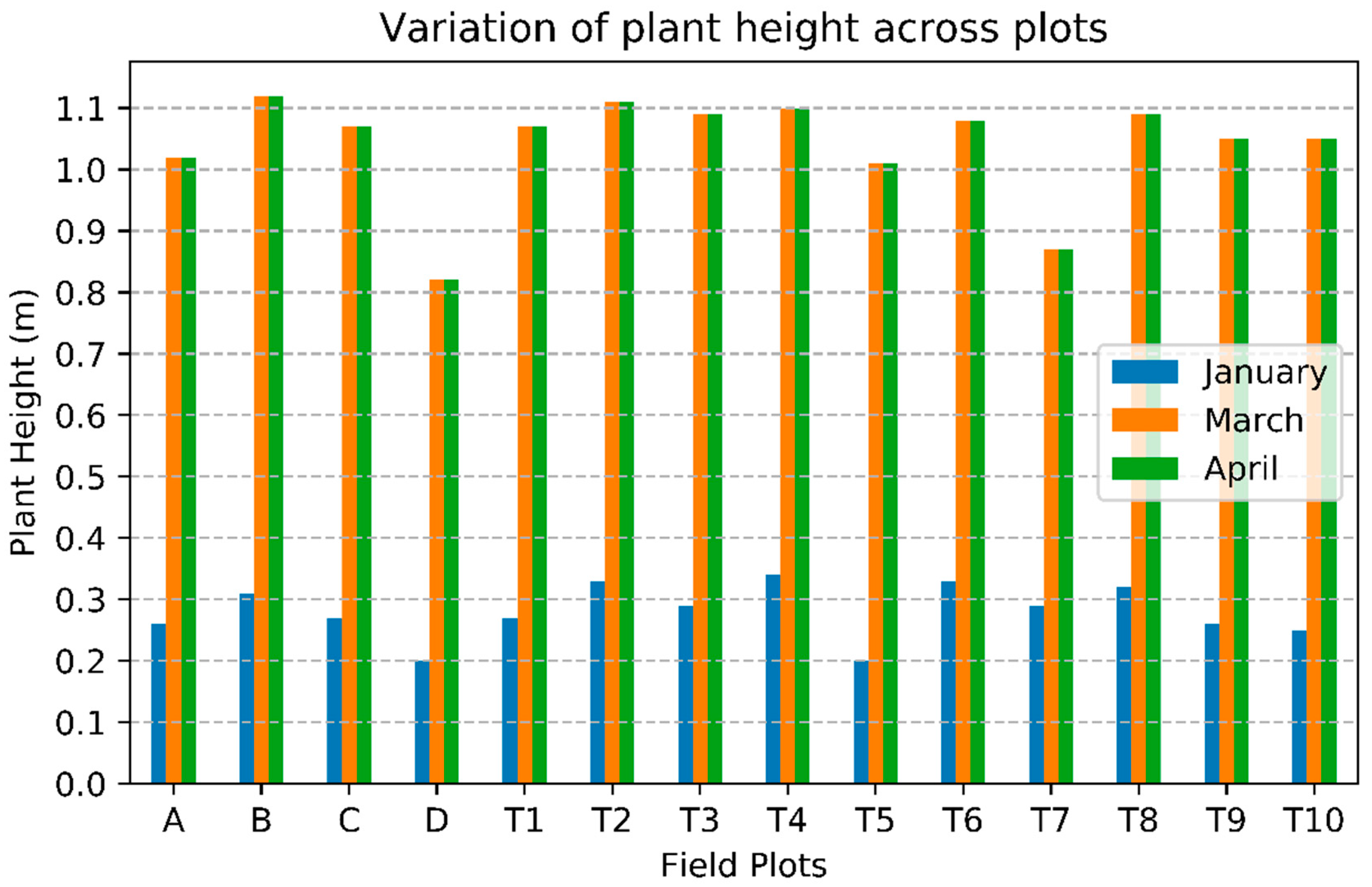
3.1. Ortho-Mosaic, CSM and Plant Height Generation
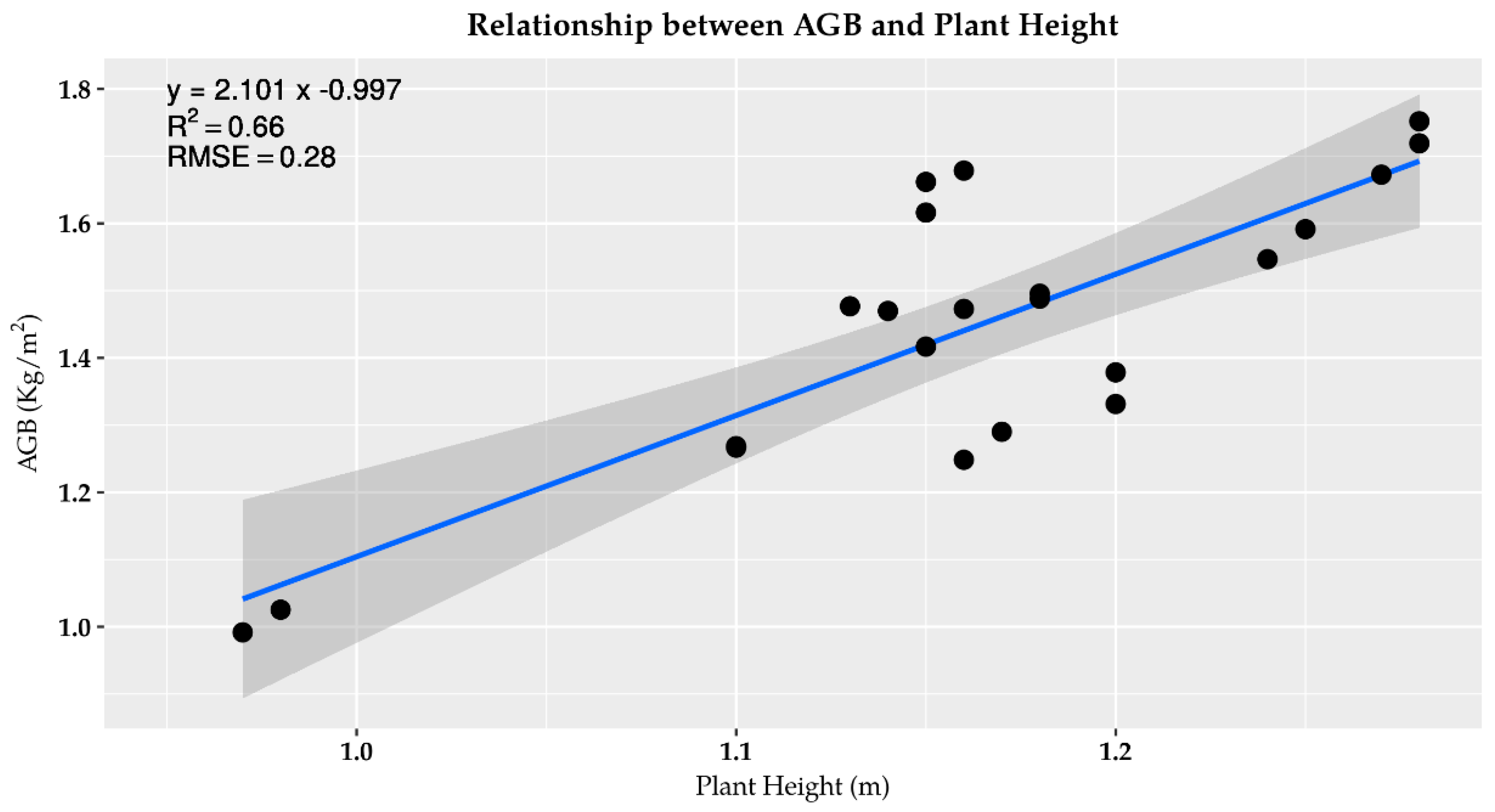
3.2. AGB Estimation
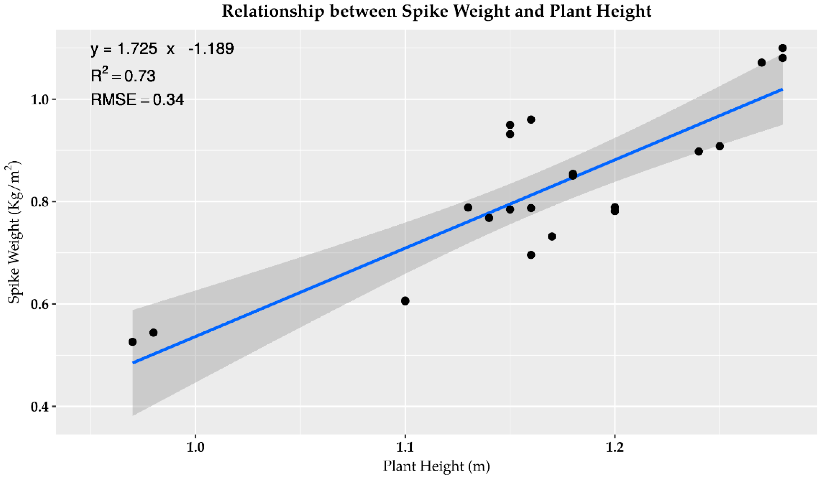
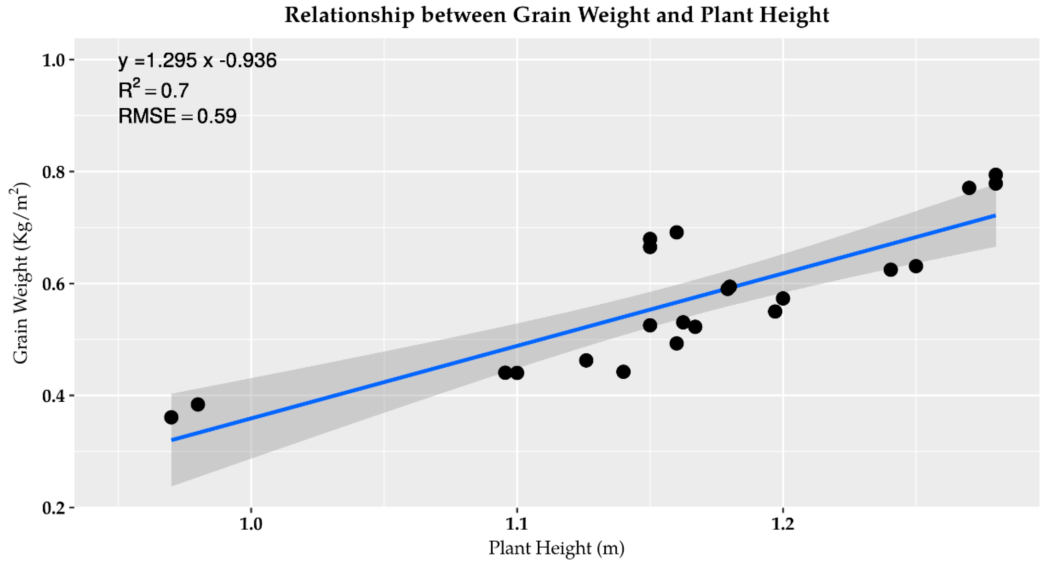
3.3. Crop Yield Estimation
4. Discussion
4.1. Data Sets and Accuracy
4.2. Cost and Scalability
5. Conclusions
Author Contributions
Funding
Acknowledgments
Conflicts of Interest
References
- Ehrlich, P.R.; Harte, J. To feed the world in 2050 will require a global revolution. Proc. Natl. Acad. Sci. USA 2015, 112, 14743–14744. [Google Scholar] [CrossRef] [PubMed] [Green Version]
- UN Sustainable Development Goals. Available online: https://www.un.org/sustainabledevelopment/sustainable-development-goals/ (accessed on 1 October 2019).
- Gomiero, T. Soil degradation, land scarcity and food security: Reviewing a complex challenge. Sustainability 2016, 8, 281. [Google Scholar] [CrossRef] [Green Version]
- Redfern, S.K.; Azzu, N.; Binamira, J.S. Rice in Southeast Asia: Facing risks and vulnerabilities to respond to climate change. Build. Resil. Adapt. Clim. Chang. Agric. Sect. 2012, 23, 295. [Google Scholar]
- Wang, H.; Hall, C.A.S.; Scatena, F.N.; Fetcher, N.; Wu, W. Modeling the spatial and temporal variability in climate and primary productivity across the Luquillo Mountains, Puerto Rico. For. Ecol. Manag. 2003, 179, 69–94. [Google Scholar] [CrossRef]
- Alexandratos, N.; Bruinsma, J. World Agriculture Towards 2030/2050: The 2012 Revision ESA Working Paper No. 12–03; Food and Agriculture Organization of the United Nations: Rome, Italy, 2012. [Google Scholar]
- Gumma, M.K.; Gauchan, D.; Nelson, A.; Pandey, S.; Rala, A. Temporal changes in rice-growing area and their impact on livelihood over a decade: A case study of Nepal. Agric. Ecosyst. Environ. 2011, 142, 382–392. [Google Scholar] [CrossRef]
- Rimal, B.; Zhang, L.; Stork, N.; Sloan, S.; Rijal, S. Urban expansion occurred at the expense of agricultural lands in the Tarai region of Nepal from 1989 to 2016. Sustainability 2018, 10, 1341. [Google Scholar] [CrossRef] [Green Version]
- FAO. Coping with Water Scarcity in Agriculture; Food and Agriculture Organization of the United Nations: Rome, Italy, 2016. [Google Scholar]
- Tilly, N.; Aasen, H.; Bareth, G. Fusion of plant height and vegetation indices for the estimation of barley biomass. Remote Sens. 2015, 7, 11449–11480. [Google Scholar] [CrossRef] [Green Version]
- Devkota, N.; Phuyal, R.K. Climatic Impact on Wheat Production in Terai of Nepal. J. Dev. Adm. Stud. 2016, 23, 1–22. [Google Scholar] [CrossRef] [Green Version]
- Family Farming Knowledge Platform—Smallholders Dataportrait. Available online: http://www.fao.org/family-farming/data-sources/dataportrait/farm-size/en/ (accessed on 3 April 2020).
- Hämmerle, M.; Höfle, B.; Höfle, B. Effects of reduced terrestrial LiDAR point density on high-resolution grain crop surface models in precision agriculture. Sensors 2014, 14, 24212–24230. [Google Scholar] [CrossRef] [Green Version]
- Lumme, J.; Karjalainen, M.; Kaartinen, H.; Kukko, A.; Hyyppä, J.; Hyyppä, H.; Jaakkola, A.; Kleemola, J. Terrestrial laser scanning of agricultural crops. In Proceedings of the International Archives of the Photogrammetry, Remote Sensing and Spatial Information Sciences—ISPRS Archives, Beijing, China, 3–11 July 2008; pp. 563–566. [Google Scholar]
- Tilly, N.; Hoffmeister, D.; Cao, Q.; Lenz-Wiedemann, V.; Miao, Y.; Bareth, G. Transferability of Models for Estimating Paddy Rice Biomass from Spatial Plant Height Data. Agriculture 2015, 5, 538–560. [Google Scholar] [CrossRef] [Green Version]
- Possoch, M.; Bieker, S.; Hoffmeister, D.; Bolten, A.A.; Schellberg, J.; Bareth, G. Multi-Temporal crop surface models combined with the rgb vegetation index from UAV-based images for forage monitoring in grassland. In Proceedings of the International Archives of the Photogrammetry, Remote Sensing and Spatial Information Sciences—ISPRS Archives, Prague, Czech Republic, 12–19 July 2016; p. 8. [Google Scholar]
- Demir, N.; Sonmez, N.K.; Akar, T.; Unal, S. Automated Measurement of Plant Height of Wheat Genotypes Using a DSM Derived from UAV Imagery. In Proceedings of the 2nd International Electronic Conference on Remote Sensing, 22 March–5 April 2018; p. 5. Available online: https://www.mdpi.com/journal/remotesensing/events/6369 (accessed on 10 June 2020).
- Colomina, I.; Molina, P. Unmanned aerial systems for photogrammetry and remote sensing: A review. ISPRS J. Photogramm. Remote Sens. 2014, 92, 79–97. [Google Scholar] [CrossRef] [Green Version]
- Melville, B.; Lucieer, A.; Aryal, J. Classification of Lowland Native Grassland Communities Using Hyperspectral Unmanned Aircraft System (UAS) Imagery in the Tasmanian Midlands. Drones 2019, 3, 5. [Google Scholar] [CrossRef] [Green Version]
- Melville, B.; Lucieer, A.; Aryal, J. Assessing the impact of spectral resolution on classification of lowland native grassland communities based on field spectroscopy in Tasmania, Australia. Remote Sens. 2018, 10, 308. [Google Scholar] [CrossRef] [Green Version]
- Adamchuk, V.I.; Ferguson, R.B.; Hergert, G.W. Soil Heterogeneity and Crop Growth. In Precision Crop Protection—The Challenge and Use of Heterogeneity; Oerke, E.C., Gerhards, R., Menz, G., Sikora, R., Eds.; Springer: Dordrecht, The Netherlands, 2010; pp. 3–16. ISBN 978-90-481-9277-9. [Google Scholar]
- Ehlert, D.; Adamek, R.; Horn, H.J. Laser rangefinder-based measuring of crop biomass under field conditions. Precis. Agric. 2009, 10, 395–408. [Google Scholar] [CrossRef]
- Bendig, J.; Bolten, A.; Bennertz, S.; Broscheit, J.; Eichfuss, S.; Bareth, G. Estimating biomass of barley using crop surface models (CSMs) derived from UAV-based RGB imaging. Remote Sens. 2014, 6, 10395–10412. [Google Scholar] [CrossRef] [Green Version]
- Niu, Y.; Zhang, L.; Zhang, H.; Han, W.; Peng, X. Estimating above-ground biomass of maize using features derived from UAV-based RGB imagery. Remote Sens. 2019, 11, 1261. [Google Scholar] [CrossRef] [Green Version]
- Acorsi, M.G.; Abati Miranda, F.D.D.; Martello, M.; Smaniotto, D.A.; Sartor, L.R. Estimating biomass of black oat using UAV-based RGB imaging. Agronomy 2019, 9, 344. [Google Scholar] [CrossRef] [Green Version]
- Zhou, X.; Zheng, H.B.; Xu, X.Q.; He, J.Y.; Ge, X.K.; Yao, X.; Cheng, T.; Zhu, Y.; Cao, W.X.; Tian, Y.C. Predicting grain yield in rice using multi-temporal vegetation indices from UAV-based multispectral and digital imagery. ISPRS J. Photogramm. Remote Sens. 2017, 130, 246–255. [Google Scholar] [CrossRef]
- Batistoti, J.; Marcato, J.; Ítavo, L.; Matsubara, E.; Gomes, E.; Oliveira, B.; Souza, M.; Siqueira, H.; Filho, G.S.; Akiyama, T.; et al. Estimating pasture biomass and canopy height in Brazilian Savanna using UAV photogrammetry. Remote Sens. 2019, 11, 2447. [Google Scholar] [CrossRef] [Green Version]
- Song, Y.; Wang, J. Winter wheat canopy height extraction from UAV-based point cloud data with a moving cuboid filter. Remote Sens. 2019, 11, 1239. [Google Scholar] [CrossRef] [Green Version]
- Adhikari, P.; Khatri-Chhetri, G.B.; Shrestha, S.M.; Marahatta, S. In-vitro study on prevalence of mycoflora in wheat seeds. J. Inst. Agric. Anim. Sci. 2015, 33–34, 27–34. [Google Scholar] [CrossRef]
- Acevedo, E.; Silva, P.; Silva, H. Wheat Growth and Physiology. Available online: http://www.fao.org/3/y4011e06.htm (accessed on 10 June 2020).
- Textbook, E. (Ed.) Introductory Statistics; OpenStax College, Rice University: Houston, TX, USA, 2013; Volume 1, ISBN 978-1-304-89164-8. [Google Scholar]
- Chai, T.; Draxler, R.R. Root mean square error (RMSE) or mean absolute error (MAE)? -Arguments against avoiding RMSE in the literature. Geosci. Model Dev. 2014, 7, 1247–1250. [Google Scholar] [CrossRef] [Green Version]
- Hunt, E.R.; Dean Hively, W.; Fujikawa, S.J.; Linden, D.S.; Daughtry, C.S.T.; McCarty, G.W. Acquisition of NIR-green-blue digital photographs from unmanned aircraft for crop monitoring. Remote Sens. 2010, 2, 290–305. [Google Scholar] [CrossRef] [Green Version]
- Berni, J.A.J.; Zarco-Tejada, P.J.; Suárez, L.; Fereres, E. Thermal and narrowband multispectral remote sensing for vegetation monitoring from an unmanned aerial vehicle. IEEE Trans. Geosci. Remote Sens. 2009, 47, 722–738. [Google Scholar] [CrossRef] [Green Version]
- Tilly, N.; Hoffmeister, D.; Cao, Q.; Huang, S.; Lenz-Wiedemann, V.; Miao, Y.; Bareth, G. Multitemporal crop surface models: Accurate plant height measurement and biomass estimation with terrestrial laser scanning in paddy rice. J. Appl. Remote Sens. 2014, 8, 083671. [Google Scholar] [CrossRef]
- Hunt, E.; Hively, W.; McCarty, G.; Daughtry, C.; Forrestal, P.; Kratochvil, R.; Carr, J.; Allen, N.; Fox-Rabinovitz, J.; Miller, C. NIR-green-blue high-resolution digital images for assessment of winter cover crop biomass. GIScience Remote Sens. 2011, 48, 86–98. [Google Scholar] [CrossRef]
- Swain, K.C.; Thomson, S.J.; Jayasuriya, H.P.W. Adoption of an unmanned helicopter for low-altitude remote sensing to estimate yield and total biomass of a rice crop. Trans. ASABE 2010, 53, 21–27. [Google Scholar] [CrossRef] [Green Version]
- Ghebregziabher, Y.T. Monitoring Growth Development and Yield Estimation of Maize Using Very High-Resolution Uav-Images in Gronau, Germany; University of Twente: Enschede, The Netherlands, 2017. [Google Scholar]
- Pix4D What Is Accuracy in an Aerial Mapping Project? Available online: https://www.pix4d.com/blog/accuracy-aerial-mapping (accessed on 14 May 2020).
- Wang, B.H.; Wang, D.B.; Ali, Z.A.; Ting Ting, B.; Wang, H. An overview of various kinds of wind effects on unmanned aerial vehicle. Meas. Control (UK) 2019, 52, 731–739. [Google Scholar] [CrossRef]
- Dandois, J.P.; Olano, M.; Ellis, E.C. Optimal altitude, overlap, and weather conditions for computer vision uav estimates of forest structure. Remote Sens. 2015, 7, 13895–13920. [Google Scholar] [CrossRef] [Green Version]
- Jin, X.; Kumar, L.; Li, Z.; Feng, H.; Xu, X.; Yang, G.; Wang, J. A review of data assimilation of remote sensing and crop models. Eur. J. Agron. 2018, 92, 141–152. [Google Scholar] [CrossRef]
- Neupane, H.; Adhikari, M.; Rauniyar, P.B. Farmers’ perception on role of cooperatives in agriculture practices of major cereal crops in Western Terai of Nepal. J. Inst. Agric. Anim. Sci. 2015, 33–34, 177–186. [Google Scholar] [CrossRef]


| Plot | Fertilizer Application/Treatment |
|---|---|
| Plot A | 120: 50: 10 Kg/ha NP2O5K2O + best management practices (BMP) Wheat variety: Bijaya [29] Sowing method: Line sowing of seeds Fertilizer application: Machine |
| Plot B | 120: 50: 10 Kg/ha NP2O5K2O + BMP Wheat variety: Bijaya Sowing method: Manual line sowing Fertilizer application: Manual line application |
| Plot C | 120: 50: 10 Kg/ha NP2O5K2O + BMP Wheat variety: Bijaya Sowing method: Precision broadcasting Fertilizer application: Precision broadcasting using Earthway spreader |
| Plot D | Fertilizer rate: Farmer practices Wheat variety: Farmer choice (local seed variety was used by the farmer) Sowing method: Farmer choice Fertilizer application: Farmer choice |
| Plot | Fertilizer Application/Treatment |
|---|---|
| T1 | 120:50:10 Kg/ha NP205K2O |
| T2 | 6-ton compost+120:50:10 Kg/ha NP205K2O |
| T3 | 6-ton farm-yard manure (FYM) +120:50:10 Kg/ha NP205K2O |
| T4 | 120:0:10 Kg/ha NP205K2O |
| T5 | 120:25:10 Kg/ha NP205K2O |
| T6 | 120:100:10 Kg/ha NP205K2O |
| T7 | 0:0:0 Kg NP205K2O /ha |
| T8 | 80:50:10 Kg NP205K2O Nitrogen from Polymer Coated Urea |
| T9 | 120:50:10 Kg NP205K2O Nitrogen from Polymer Coated Urea |
| T10 | 120:50:10 Kg NP205K2O + 10 ton/ha Rice fly ash |
| Growth Stage [30] | Days after Sowing | Flight Date | No. of Images | Remarks |
|---|---|---|---|---|
| 13 | 8 December 2017 | 46 | As the zoom level of background images for flight planning was low, flight plans were prepared based on an educated guess thereby varying the area (and the number of images) covered. | |
| Terminal spikelet | 42 | 6 January 2018 | 62 | |
| Heading | 105 | 10 March 2018 | 79 | |
| Physiological maturity | 130 | 4 April 2018 | 60 |
| Image Acquisition Date | RMSE (m) |
|---|---|
| 8 December 2017 | 0.02 |
| 6 January 2018 | 0.02 |
| 10 March 2018 | 0.03 |
| 4 April 2018 | 0.03 |
| Plot | Field Measured AGB (Kg/m2) | Estimated AGB (Kg/m2) | Error (%) |
|---|---|---|---|
| T9 | 1.526 | 1.357 | 11.0 |
| T9 | 1.565 | 1.379 | 11.9 |
| T10 | 1.726 | 1.505 | 12.8 |
| T10 | 1.761 | 1.526 | 13.4 |
| C | 1.389 | 1.526 | −9.8 |
| C | 1.377 | 1.505 | −9.3 |
| C | 1.418 | 1.526 | −7.6 |
| D | 1.095 | 1.084 | 1.0 |
| D | 1.186 | 1.084 | 8.6 |
| D | 1.091 | 1.063 | 2.6 |
| Plot | Spike Weight (Kg/m2) | Grain Weight (Kg/m2) | Remarks | ||||
|---|---|---|---|---|---|---|---|
| Field Measured | Estimated | Error (%) | Field Measured | Estimated | Error (%) | ||
| T9 | 0.838 | 0.744 | 11.2 | 0.600 | 0.515 | 14.3 | |
| T9 | 0.852 | 0.762 | 10.6 | 0.612 | 0.527 | 13.8 | |
| T10 | 0.918 | 0.865 | 5.8 | 0.553 | 0.605 | −9.4 | |
| T10 | 0.932 | 0.882 | 5.3 | 0.625 | 0.618 | 1.1 | |
| C | 0.876 | 0.882 | −0.7 | 0.651 | 0.618 | 5.1 | |
| C | 0.892 | 0.865 | 3.0 | 0.632 | 0.605 | 4.2 | |
| C | 0.911 | 0.882 | 3.1 | 0.665 | 0.618 | 7.1 | |
| D | 0.673 | 0.520 | 22.8 | 0.473 | 0.346 | 26.8 | Use of local seed variety. Inclusion of bare soil height and height of weeds with smaller heights besides wheat plants, in a CSM grid. |
| D | 0.650 | 0.520 | 20.0 | 0.450 | 0.346 | 23.1 | |
| D | 0.604 | 0.503 | 16.8 | 0.439 | 0.333 | 24.1 | |
© 2020 by the authors. Licensee MDPI, Basel, Switzerland. This article is an open access article distributed under the terms and conditions of the Creative Commons Attribution (CC BY) license (http://creativecommons.org/licenses/by/4.0/).
Share and Cite
Panday, U.S.; Shrestha, N.; Maharjan, S.; Pratihast, A.K.; Shahnawaz; Shrestha, K.L.; Aryal, J. Correlating the Plant Height of Wheat with Above-Ground Biomass and Crop Yield Using Drone Imagery and Crop Surface Model, A Case Study from Nepal. Drones 2020, 4, 28. https://doi.org/10.3390/drones4030028
Panday US, Shrestha N, Maharjan S, Pratihast AK, Shahnawaz, Shrestha KL, Aryal J. Correlating the Plant Height of Wheat with Above-Ground Biomass and Crop Yield Using Drone Imagery and Crop Surface Model, A Case Study from Nepal. Drones. 2020; 4(3):28. https://doi.org/10.3390/drones4030028
Chicago/Turabian StylePanday, Uma Shankar, Nawaraj Shrestha, Shashish Maharjan, Arun Kumar Pratihast, Shahnawaz, Kundan Lal Shrestha, and Jagannath Aryal. 2020. "Correlating the Plant Height of Wheat with Above-Ground Biomass and Crop Yield Using Drone Imagery and Crop Surface Model, A Case Study from Nepal" Drones 4, no. 3: 28. https://doi.org/10.3390/drones4030028