An Open Simulation Strategy for Rapid Control Design in Aerial and Maritime Drone Teams: A Comprehensive Tutorial

Abstract

The deployment of robot controllers into the real robotic platform is cumbersome and time consuming, especially when testing scenarios involve several robots or are sites not easily accessible. Besides this, most of the time, testing on the real platforms or real conditions provides little value in the early stages of controller design and prototype, phases where debugging and suitability of the controller are the main objectives. This paper proposes a simulation strategy for developing and testing controllers for Unmanned Aerial and Surface Vehicle coordination and interaction with the environment. The simulation strategy is based on V-REP and Matlab/Simulink which provide a large set of features, modularity and compatibility across platforms. Results show that this approach significantly reduces development and delivery times by providing an off-the-shelf simulation environment and a step-by-step implementation guidelines. The source code to deploy the simulations is available in an open-source repository.

1. Introduction

As remote sensing techniques become increasingly popular, unmanned robots such as aerial and surface vehicles (UAV and USV) are making their way into diverse fields by providing access to new technology approaches to data collection along with the augmented accessibility provided by these platforms [1,2]. This application of unmanned robots can be used to access dangerous sites or places where traditional manned sensing techniques are impossible to implement, and are being widely adopted in various fields such as [3,4,5].

One of the fields where UAV and USV applications have kicked off is limnology, the branch of science that studies inland aquatic ecosystems [6]. In limnological studies manual sampling techniques are usually tedious or sometimes dangerous to perform. And the commonly lead to an increased probability of inaccurate or faulty results due to erroneous field practices [1]. Besides this, autonomous platforms tend to provide a reliable permanent record of the measured conditions which makes revisiting and comparison over time possible and effortless.

Obtaining extensive and reliable on site limnological data within short delivery time windows and tight operational budgets is one of the main advantages of the application of unmanned robots in the field. This quality assessment of inland waters is directly in line with one of the main biodiversity and habitat conservation action fields launched by European 2020 biodiversity policies [7].

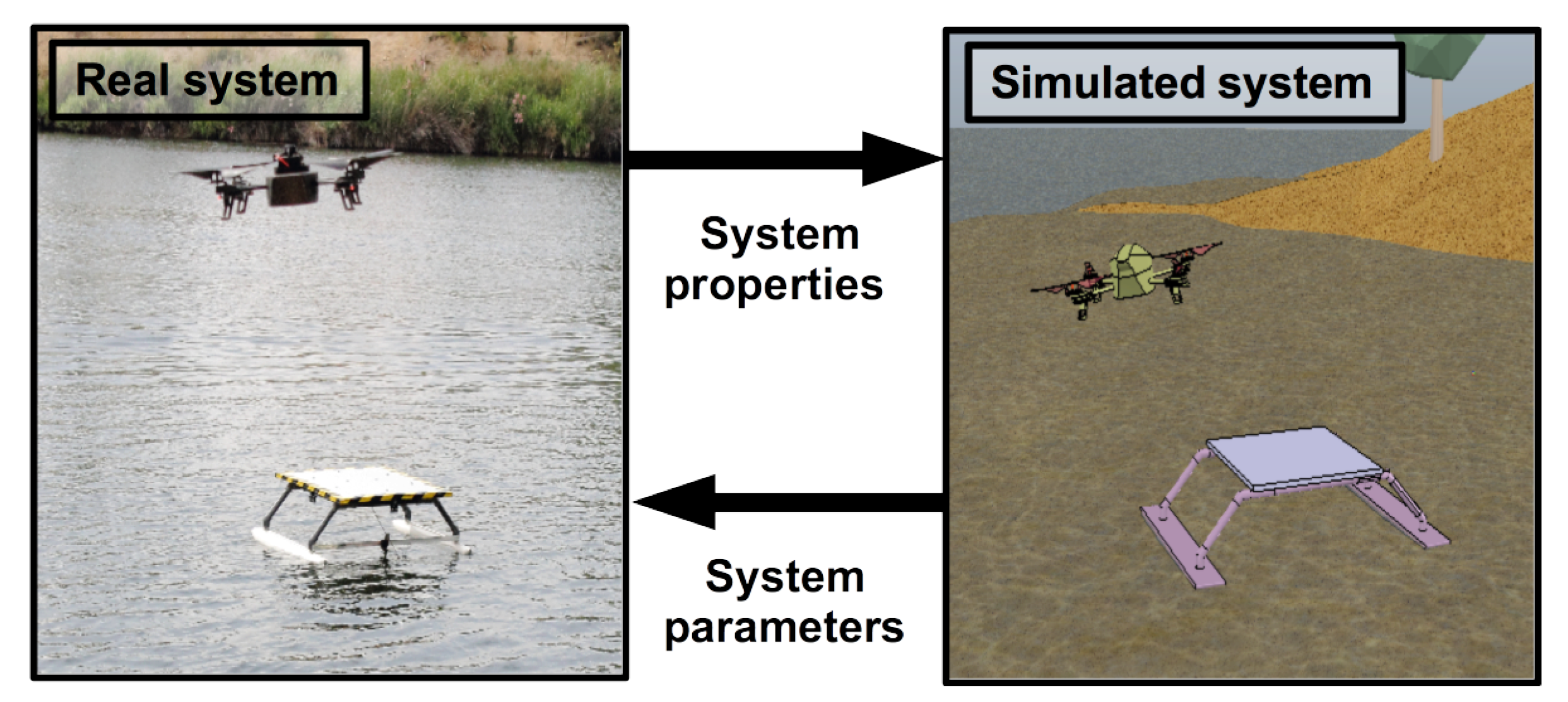
This work presents a simulation strategy for a collaborative scheme between an autonomous surface vehicle and an autonomous aerial vehicle. The objective of this multi-robot solution is to provide a collaboration system to perform data collection tasks from calm water environments in the frame of limnology studies. The selected aerial platform is based on the AR.Drone quadcopter while the surface vehicle, the Strider V1.0, a catamaran vessel, is a prototype platform developed specifically for this project [8] (see Figure 1).

The USV acts as a mobile landing platform for the drone where on deck charging of the UAV battery can be done. The UAV’s flexibility of operations allows the access to zones where the surface vehicle cannot reach, along with different types of aerial surveys [9]. While the USV performs this “piggybacking” duty, it can also be equipped with several surface based survey equipment to complement and expand the data pool.

The main objective of this work is to provide a simulation strategy to prototype and quickly test control strategies where interaction between the robots and the environment is needed. The ability to test and prototype control architectures, path planning algorithms and sensors allows development and deployment times in missions to be reduced. This also allows for better and more reliable data acquisition by reducing the failure rate in missions due to invalid and/or inadequate approaches to limnological sampling. This simulation strategy will provide a portable and flexible solution across different platforms.

2. Related Work

With the recent wake in drone and multicopter popularity a lot of specific simulators for UAVs can be found, for professional, research and commercial purposes. Most of the commercially oriented simulators are aimed at hobbyists and gamers [10,11], while professional simulators tend to be simulation platforms for training and simulating missions, mostly in the military field [12,13]. These simulators tend to be provided only with direct flight of the quadcopter. This basic control is implented through the usual quadcopter joystick controllers without any other control implementation or access to the internal states of the quadcopter [14].

Most of the UAV research oriented simulators are built into physics and visualization engines that provide the ability to complete knowledge of the simulation environment and states. Some of these research simulator examples can be found in [15] with a simulator based on Unreal Engine 4 or [16] using the low fidelity quadcopter included in V-REP. Another example is [17], based on the Gazebo simulator and used in the tum_Simulator [18] package, that uses it along the ardrone_autonomy package as a driver to simulate the Parrot Ar.Drone quadcopter.

USV simulation faces a similar panorama as its UAV counterpart. Most of the professional software is aimed at design prototyping and dynacmic studies in product development phases and usually have a higher cost of access. On the other hand commercial/hobbyist simulators usually do not provide the necessary model accuracy needed for control prototyping due to the difficulty of hydrodynamic effects and interactions.

Some examples are the VeSim Simulator developed by Sintef, and also some packages for the Gazebo simulator can be found for USV simulation such as the Kingfisher/Heron USV package. The lack of easily accessible USV simulators that can be operated outside professional or military uses and involve interaction with the environment is notable. There are some scarce examples such as [19,20] which are set up only for USV simulation, and [21], framed in the RIVERWATCH project. The RIVERWATCH project is one of the notable UAV-USV multi-robot teams for riverine environments, and their simulations are based on Robot Operating System (ROS) and Gazebo. More recently, in Paravisi et al. the authors present a gazebo-based simulation environment that models waves, wind, and water currents. The simulator also provide four USV and real scenario models. The authors enhance the lack of research on USV control strategies and the need to develop further USV navigation strategies [22].

Although some of the simulators mentioned above are provided with model simulations for their respective platforms, the ones built on robotic simulators (such as V-REP and Gazebo among others), are the only simulation platforms that allow easy implementation and simulation of multiple robotic platforms over already existing models thanks to their capabilities. The ability to independently control and quickly develop, prototype and deploy robotic experiments provided by this type of simulation strategy makes it a valuable asset in most research environments and drastically reduces result delivery times.

In particular, the selection of V-REP over a Gazebo based implementation (such as the aforementioned [21]), is based on the different set of features that each software includes:

Some of the most relevant features of V-REP over Gazebo, are its ability to import CAD models and its mesh manipulation and edition tools that allow their quick transformation into usable and efficient robotic models. It also features more physics engines by default, multiple simulation output formats, compatibility with various programming languages and includes particle systems. Furthermore, V-REP’s easy integration with other services through external API implementations and ROS immediately expands the usability of these simulation strategies thanks to the widespread presence of ROS in the robot industry and research field.

Besides, V-REP provides a more robust execution, opposed to the sometimes common freezes in Gazebo, it is more intuitive, has a very well documented API and a wide cross platform compatibility. Overall, V-REP packs more features by default while a similar featured Gazebo installation relies in a large set of external tools, however its main trade-off against Gazebo or other simulators is the increased computational requirements, which limits its use in real time complex simulations.

A further and more thorough comparison can be found in [23,24] where a summary and evaluation of both simulators is given.

3. Dynamic Modeling

This section covers the dynamic modeling of the UAV and USV selected for this work. In this case the UAV selected is the AR.Drone 2.0 quadcopter, although the same obtained model can be applied to any other quadcopter. The USV selected is the Strider V1.0 vessel as mentioned before.

Considering the scope of the simulation environment, a set of assumptions are taken into account concerning both robotic systems. In the case of the quadcopter, the following typical assumptions are considered in order to simplify the modelling task:

• The body-fixed frame axes coincide with the principal axes of inertia of the body
• The moments of inertia are constant.
• The body-fixed frame origin $o_B$ is coincident with the centre of mass.
• Body symmetry with respect to the centre of mass is assumed.
• Minor aerodynamic effects such as blade flapping or induced drag are not considered.

For the modelling of the Strider V1.0 manoeuvring theory [25], which concerns motion of the vessel at slowly varying or constant speeds, is adopted. In Manoeuvring Theory, only surge, sway and yaw motions are considered and calm and restricted waters assumed. Assumptions 1 to 4 coincide with the ones made for the UAV model, and are complemented by the following:

6.

Restricted, calm and still water bodies is assumed. This implies that no currents or waves affect the motion of the ship.

7.

Heave, roll and pitch motions are neglected due to a zero frequency wave excitation assumption.

8.

Surge motion is decoupled from sway and yaw motion due to the symmetry of the vessel hulls.

9.

Added mass effects on the hulls are neglected since only steady motion will be considered.

3.1. Uav Modeling

Concerning quadcopter modeling, an inertial and a fixed-body frame is defined, following the notation in Figure 2, where E is the inertial earth frame and B is the fixed-body frame, attached to the quadcopter airframe and along the arms of the quadrotor.

Let us then define the following workspace within this two frames. Two vectors can be defined to give a generalized overview of the position and velocity of the quadrotor in the space:

$$\xi ={\left[\begin{array}{cc}{\Gamma }^E& {\Theta }^E\end{array}\right]}^T={\left[\begin{array}{cccccc}x& y& z& \varphi & \theta & \psi \end{array}\right]}^T$$

(1)

$$\nu ={\left[\begin{array}{cc}{\mathbf{V}}^B& {\mathit{\omega }}^B\end{array}\right]}^T={\left[\begin{array}{cccccc}u& v& w& p& q& r\end{array}\right]}^T$$

(2)

where $\xi [+]$ represents the generalized position of the body in terms of the earth frame. and $\mathit{\nu }[+]$ the generalized velocity in terms of the body frame. The vector ${\mathbf{V}}^B$ [m s${}^{-1}$] represents the linear velocity vector of the body frame with respect to the inertial frame, being $u,v$ and $\omega$ the velocities in the positive $x_B$, $y_B$ and $z_B$ directions respectively. Similarly, the vector ${\mathit{\omega }}^B$ [rad s${}^{-1}$] represents the angular velocity of the quadrotor with respect to the inertial frame, being $p,q$ and r the angular velocities around the $x_B$, $y_B$ and $z_B$ axes. ${\Gamma }^E$ [m] and ${\Theta }^E$ [rad] represent the linear and angular position, being $x,y\mathrm{and}z$ the position of the body frame with respect to the earth frame and $\varphi$ stands for roll, $\theta$ for pitch and $\psi$ for yaw of the body frame with respect to the inertial frame.

The rigid body dynamic equations of the quadrotor after the previously made assumptions come from the application of Newton’s second law, according to Equation (3):

$$\begin{array}{cc}\hfill m{\ddot{\mathit{\Gamma }}}^E& ={\mathbf{F}}^E\hfill \\ \hfill m\dot{\widehat{{\mathbf{R}}_{\Theta }{\mathbf{V}}^B}}& ={\mathbf{R}}_{\Theta }{\mathbf{F}}^B\hfill \\ \hfill m({\mathbf{R}}_{\Theta }{\dot{\mathbf{V}}}^B+{\dot{\mathbf{R}}}_{\Theta }{\mathbf{V}}^B)& ={\mathbf{R}}_{\Theta }{\mathbf{F}}^B\hfill \\ \hfill m{\mathbf{R}}_{\Theta }({\dot{\mathbf{V}}}^B+{\mathit{\omega }}^B\times {\mathbf{V}}^B)& ={\mathbf{R}}_{\Theta }{\mathbf{F}}^B\hfill \\ \hfill m({\dot{\mathbf{V}}}^B+{\mathit{\omega }}^B\times {\mathbf{V}}^B)& ={\mathbf{F}}^B\hfill \end{array}$$

(3)

where m [Kg] is the mass of the quadrotor, ${\ddot{\mathit{\Gamma }}}^E$ [m s${}^{-2}$] is the second derivative of the linear position of the body frame with respect to the earth frame, ${\mathbf{F}}^E$ [N] and ${\mathbf{F}}^B$ [N] are the forces vector with respect to the earth and body frame, ${\mathbf{R}}_{\Theta }$ is the rotation matrix and ${\mathbf{V}}^B$ and ${\mathit{\omega }}^B$ are the body frame linear and angular speeds of the quadrotor expressed in the body frame.

Similarly, we can develop the angular components of this motion equations:

$$\begin{array}{cc}\hfill \mathbf{I}{\ddot{\Theta }}^E& ={\mathit{\tau }}^E\hfill \\ \hfill & ⋮\hfill \\ \hfill \mathbf{I}\dot{{\mathit{\omega }}^B}+{\mathit{\omega }}^B\times (\mathbf{I}{\mathit{\omega }}^B)& ={\mathbf{⌀}}^B\hfill \end{array}$$

(4)

where $\mathit{I}$ [N m s${}^2$] is the inertia matrix of the body (with respect to the body frame), ${\ddot{\Theta }}^E$ [rad s${}^{-2}$] is the second derivative of the angular position of the quadrotor with respect to the earth frame, ${\mathit{\tau }}^E$ [N m] and ${\mathit{\tau }}^B$ [N m] are the torques vectors with respect to the earth and body frame.

Equations (3) and (4) are the generic expressions of Newton’s second law in a three dimensional space for a 6-DOF rigid body. Equation (5) expresses this two equations in matrix form. This matrix equation represents the generalized expression for the motion of any rigid body based on the assumptions made before.

$$\left[\begin{array}{cc}m{\mathit{I}}_{\mathbf{3}\times \mathbf{3}}& {\mathbf{0}}_{\mathbf{3}\times \mathbf{3}}\\ {\mathbf{0}}_{\mathbf{3}\times \mathbf{3}}& \mathit{I}\end{array}\right]\left[\begin{array}{c}{\dot{\mathbf{V}}}^B\\ {\dot{\mathit{\omega }}}^B\end{array}\right]+\left[\begin{array}{c}{\mathit{\omega }}^B\times (m{\mathbf{V}}^B)\\ {\mathit{\omega }}^B\times (\mathit{I}{\mathit{\omega }}^B)\end{array}\right]=\left[\begin{array}{c}{\mathbf{F}}^B\\ {\mathit{\tau }}^B\end{array}\right]$$

(5)

We can characterize this expression to the quadcopter model by defining the force and torque vector at the right side of the equation. In the case of the quadcopter model, this force and torque vector can be divided into four basic components: gravitational, propeller’s thrust, gyroscopic effects and exogenous forces [26].

3.2. Usv Modeling

For the dynamic modeling of the Strider V1.0 a similar rigid-body mechanical model to the one used in the previous section is adopted. An inertial and a body fixed frame will be defined to create a suitable workspace for the model. The SNAME (Society of Naval Architects and Marine Engineers) provides a standard notation and sign convention for the description of the motion of ships shown in Figure 3.

An inertial earth frame, following the NED convention, and a fixed-body frame, attached to the vehicle’s platform, are defined following the notation shown in Figure 3. Generally for surface ships the centre position for the body fixed frame is located in such a way that it gives hull symmetry about the $x_0-z_0$ plane and approximate symmetry about the $y_0-z_0$ plane while the origin of the $z_0$ axis is set on the calm water surface. In the particular case of this work, due to the symmetry and small size of platform, the hydrodynamic forces and moments acting on the ship can be easily described when the centre of the body-frame is coincident with the centre of gravity of the vessel. Thus, the position of $O_0$ will be assumed to be located at the centre of mass of the Strider V1.0. With this in mind the following notation will be used.

$$\begin{array}{cc}\hfill {\mathit{\eta }}^E& ={\left[\begin{array}{cc}{\Gamma }_{Str}^E& {\Theta }_{Str}^E\end{array}\right]}^T={\left[\begin{array}{cccccc}x& y& z& \varphi & \theta & \psi \end{array}\right]}^T\hfill \end{array}$$

(6)

$$\begin{array}{cc}\hfill {\mathit{\nu }}^B& ={\left[\begin{array}{cccccc}u& v& w& p& q& r\end{array}\right]}^T\hfill \end{array}$$

(7)

$$\begin{array}{cc}\hfill {\mathit{\tau }}^B& ={\left[\begin{array}{cccccc}X& Y& Z& K& M& N\end{array}\right]}^T\hfill \end{array}$$

(8)

where ${\mathit{\eta }}^E[+]$ is the linear and angular position with respect to the inertial frame, ${\mathit{\nu }}^B[+]$ the linear and angular velocity of the ship with respect to the body frame and ${\mathit{\tau }}^B[+]$ represents the forces and torques applied to the body in terms of the body fixed frame.

Following the assumptions made in the previous section we can propose the following 3DOF dynamic model of the vessel, considering it as single rigid body system:

$$\left[\begin{array}{ccc}m& 0& 0\\ 0& m& 0\\ 0& 0& I_z\end{array}\right]\left[\begin{array}{c}\dot{u}\\ \dot{v}\\ \dot{r}\end{array}\right]+\left[\begin{array}{ccc}0& -mr& 0\\ mr& 0& 0\\ 0& 0& 0\end{array}\right]\left[\begin{array}{c}u\\ v\\ r\end{array}\right]=\left[\begin{array}{c}X\\ Y\\ N\end{array}\right]$$

(9)

We can characterize this expression to the Strider V1.0 model by defining the forces and torques at play in the motion of the vessel. In the case of the Strider V1.0 model, this force and torque vector can be divided into three components: the hydrodynamic effects modeled using the approach in [27], control surfaces and propulsion and external forces.

4. Simulation Approach

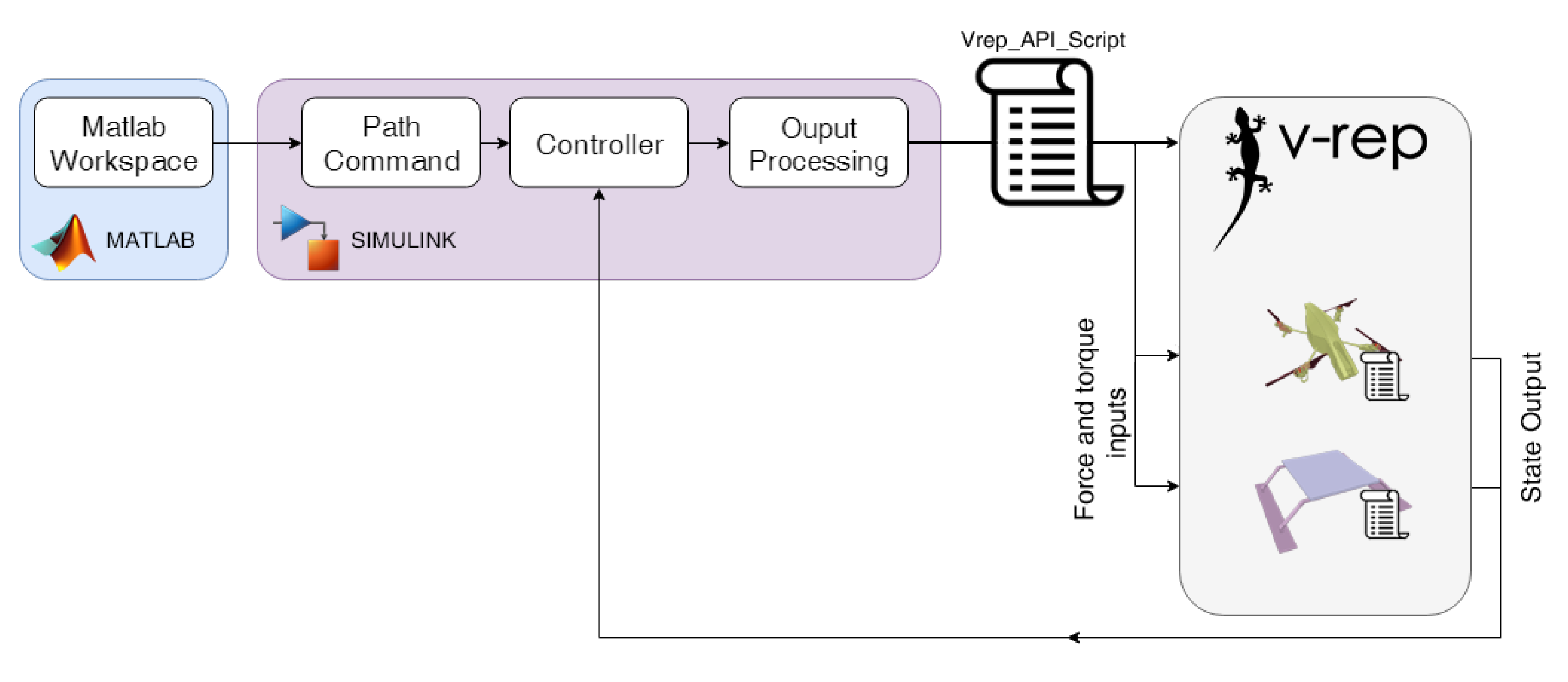
The simulation strategy used in this work is based on Simulink and the V-REP robot simulator. Although the performed simulations detailed in the experimental section of this paper were made using a Windows 10 machine, both Matlab and V-REP provide great compatibility and portability among different OS. This simulation strategy can be run independently of the machine’s OS or auxiliary software since the communication interface between both programs is achieved by means of the V-REP’s supported external API.

Simulink provides the controller and processing architecture and outputs the forces and torques to be applied to the rigid body system. Rigid body and physics simulations are provided by any of the included physic engines in VREP, which also provides a visualization environment. A more in depth description of these software platforms and their operation for the implementation of the simulation strategy is covered in the next sections. Matlab–V-REP interaction is handled through a Matlab S-function block written in C, interfacing through the remote V-REP API for C language as can be seen in the scheme shown in Figure 4.

The chosen software (shown in

Table 1. Used software and addons.

Software	Version	License	Description
Matlab	2017b	Academic license	Simulation environment
Simulink	9.0 (R2017b)	Academic license	Simulation environment
V-REP	3.4.0 (rev 1)	GNU GPL	Robot simulation environment
Vortex Studio Essentials	2017.2.0.64	Freeware	Physics engine addon

) provides great compatibility with ROS for future hardware in the loop implementations and real world test. Matlab has an integrated toolbox (“Robotic System Toolbox”) which provides support for ROS, and also direct support for the Ar.Drone 2.0 via its embedded coder [28]. V-Rep also features a ROS interface, based on the C/C++ ROS API which allows communication via ROS.

4.1. Processing and Command

As it can be seen from Figure 4, the majority of the processing and the command input and simulation pace control is made in Matlab and Simulink.

In this application, Simulink (Version 9.0 (2017b)) was used to build the control architecture and the processing and communication blocks to allow and control the data flow between V-REP and Simulink. A screenshot of the Simulink built architecture can be seen in Figure 5.

In Figure 5 purple subsystems contain the path command blocks that read the necessary data from the Matlab workspace. In the case of the quadcopter block, it also contains the block implementation of the simple VTOL algorithm implemented to govern the commanded altitude. Orange subsystems contain the controller architectures for both robotic platforms. The ones pertaining to the quadcopter include the two variant implemented control architectures (a cascaded PID and an Inverse Kinematics architecture). Next, green subsystems enclose the processing of the output of the controllers and translate them to the forces and torques to be applied to the robot models in V-REP. This is where the dynamic models of the robots calculated in the previous section are used.

Finally, the output of the green subsystems gets fed to the V-REP block. This block contains the interfacing S-function, that receives as an input a vector of fourteen elements:

$$input=[F^B{}^{\prime }{\tau }^B{}^{\prime }Th{}^{\prime }{X}_{rudder}{}^{\prime }{Y}_{rudder}{}^{\prime }X{}^{\prime }Y{}^{\prime }N{}^{\prime }]$$

(10)

Being the first two elements the thrust and torque of each of the propellers of the quadcopter and the rest the thrust, rudder and hydrodynamic and exogenous forces and torque acting on the Strider V1.0. The apostrophe (${}^{\prime }$) denotes the transpose of the vectors.

The V-REP block also outputs the state of the robots to provide the necessary feedback for the controller and data collection. The output format of the block is:

$$\begin{array}{c}output=\left[\begin{array}{cccccc}\xi {}^{\prime }& V^B{}^{\prime }& {\dot{V}}^B{}^{\prime }& {\Gamma }_{Str}^E{}^{\prime }& {v^B}^{\prime }& \psi {}^{\prime }\end{array}\right]\end{array}$$

(11)

Being the first three elements the position, velocity and accelerations of the quadcopter and the rest the position, velocity and yaw angle of the Strider V1.0.

4.2. Physics, Sensor Simulation and Visualization

V-REP is a robot simulator environment developed by Coppelia Robotics and it implements the physics and sensor simulation in this approach. It allows for individual control of different object and models and features a wide arrange of programming and interacting environments such as ROS, plugins, embedded scripts or remote API solutions in several programming languages, making it a versatile software for multirobot simulation and interaction.

Along the multiple features of V-REP it allows to simulate a wide array of realistic sensors such as vision or proximity sensors. This allows for a more accurate and complete representation of the simulated robotic systems and easier development and testing. Figure 6 shows a screenshot of the simulator in V-REP in a setup scene.

V-REP was chosen in this work due to its easy API integration and its compatibility along different platforms and portability.

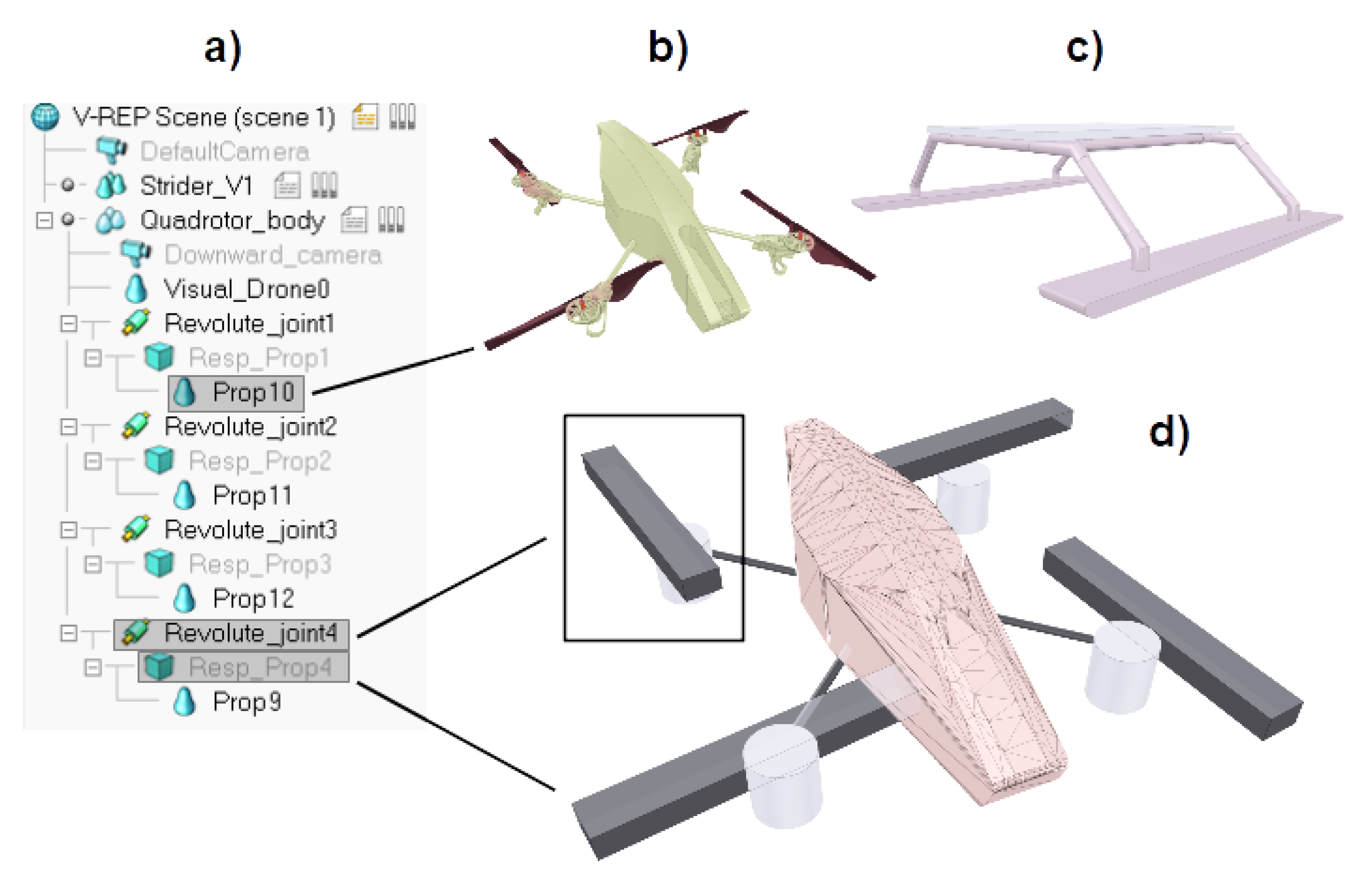
The implementation of the robotic model is generally straightforward but it usually requires some time to simplify and optimize the model for simulation. This involves a series of steps to be followed to obtain the models of the robots in the simulation environment:

(1)

The models of both robots have to be imported into the V-REP environment. This can be done by importing a pre-existing CAD model of the robot or by building it directly in V-REP, which can be later simplified to improve significantly simulation speed.

(2)

After the import of the CAD models and their simplification, it is necessary to configure the shape’s properties and the hierarchical relationship between them to build an operational robot model for simulation. These shapes are usually divided into a visual and respondable (collision and dynamically enabled) pair. An example of this model building structure can be seen in Figure 7, where the visual appearance of the robot, and the respondable and dynamic shapes are compared side by side.

(3)

The implementation of the robotic models in V-REP, where the communication and behaviour of each of the robot models has to be set. This is achieved by embedded scripts attached to each model. These scripts handle the external API functions in order to receive and send the commands and current states. After that, it applies these received commands as forces and torques in the appropriate locations. These embedded scripts are written in Lua and an example is shown in Figure 8.

Communications between the client (Matlab) and the server (V-REP) runs in synchronous mode, that is, the next simulation pass in V-REP does not get started until a trigger signal is sent by the client side. This ensures correct functioning and synchronization between the two parallel simulation processes (simulink & V-REP) since the processing time of each simulation step in both platforms is not the same. This way, once the client side is ready to initiate another simulation pass, after the processing of the received and output data, it triggers the start of a new simulation pass.

4.3. Parametrization of the Simulation

After the description of the dynamic models of both the UAV and the USV we can define the forces that will be taken into account for each model:

In the case of the quadcopter only the contribution from the propellers will be explicitly introduced into the model since gravitational and simple gyroscopic effects are already included in the simulation engines. The forces corresponding to the thrusts and torques of each of the propellers is applied at the centre of each of the four rotors. Exogenous forces, if considered, are applied directly to the centre of mass of the quadcopter.

For the vessel model, all the described force and torque contributions will be explicitly introduced in. In the case of Hydrodynamic Forces, the expressions from [27] can be simplified by neglecting added mass (because of the made assumptions) and rudder component terms (due to the addition of a more precise rudder model) to the model resulting in:

$$\begin{array}{cc}Y\hfill & =Y_{v}v+Y_{r}r\hfill \end{array}$$

(12)

$$\begin{array}{cc}N\hfill & =N_{v}v+N_{r}r\hfill \end{array}$$

(13)

both Hydrodynamic and exogenous forces are applied to the centre of mass of the vessel. Rudder forces and propeller are applied at the Centre of pressure of the rudder $C{P}^B$ and the centre of the propeller respectively.

For both the quadrotor and the vessel simulation, solid geometry, mass and inertia properties have been directly imported from the existing CAD models.

Table 2. Simulation Parameters.

Platform	Variable	Value
AR.Drone	$c_T$	$9.14\dot{1}{0}^{-6}$
	$c_D$	$2.38\dot{1}{0}^{-9}$
	Max. propeller rpm	5000 rpm
Strider V1.0	$Y_v$	$-3.89950$
	$Y_r$	$1.77427$
	$N_v$	$-1.77427$
	$N_r$	$-0.80729$
	$x_{cp}-x_{cg}$	0.347 m
	Air drag coefficient	$0.2$
	Rudder lift coefficient	$1.2$
	Rudder area	0.0064 m${}^2$
	Water density	998 Kg m${}^{-3}$

provides the data concerning the rest of variables not parametrized in the CAD models such as lift and drag coefficients and the value of the hydrodynamic derivatives.

Some of the parameters of the simulation have been obtained from external sources [29,30,31,32]. Detailed sourcing and comments on them is given below.

The data for the maximum RPM of the rotors along with the values for the thrust $C_T$ and drag $C_D$ coefficients have been obtained from [29,30]. Both works present empirical results from model identification tests of the AR.Drone 2.0. The values of the hydrodynamic derivatives have been obtained from the expressions from [31].

Rudder lift coefficient is estimated based on the works of [32], where a general guideline based on experimental results gives good estimations on lift coefficient in spade rudders.

Air drag coefficients for the vessel model have been obtained from the work made during the development of the Strider V1.0 prototype.

Concerning the addition of more UAV or USV models to the simulation, the same architecture scheme shown in Figure 5 could get replicated and run in parallel in the same model for each robot pair, and small call modifications in the interfacing code for the calling of the new robots embedded scripts included. Because of the modularity of this approach it is also possible to only duplicate the Matlab S-function block with the necessary modifications to the remote API script to control another robot/s.

5. Control Architecture

This section presents the controller that enables the vehicles attitude and position control, the minimum system requisites for vehicle autonomous navigation. The modularity of the Simulink model allows for easy implementation of other control architectures by simply plugging directly into the desired control stage of the architecture. Controllers were tuned during simulation using the provided tools in Simulink.

5.1. Quadcopter Control

The quadcopter controller architecture features two different swappable controllers. Both controllers are described next.

5.1.1. Cascaded Pid Architecture

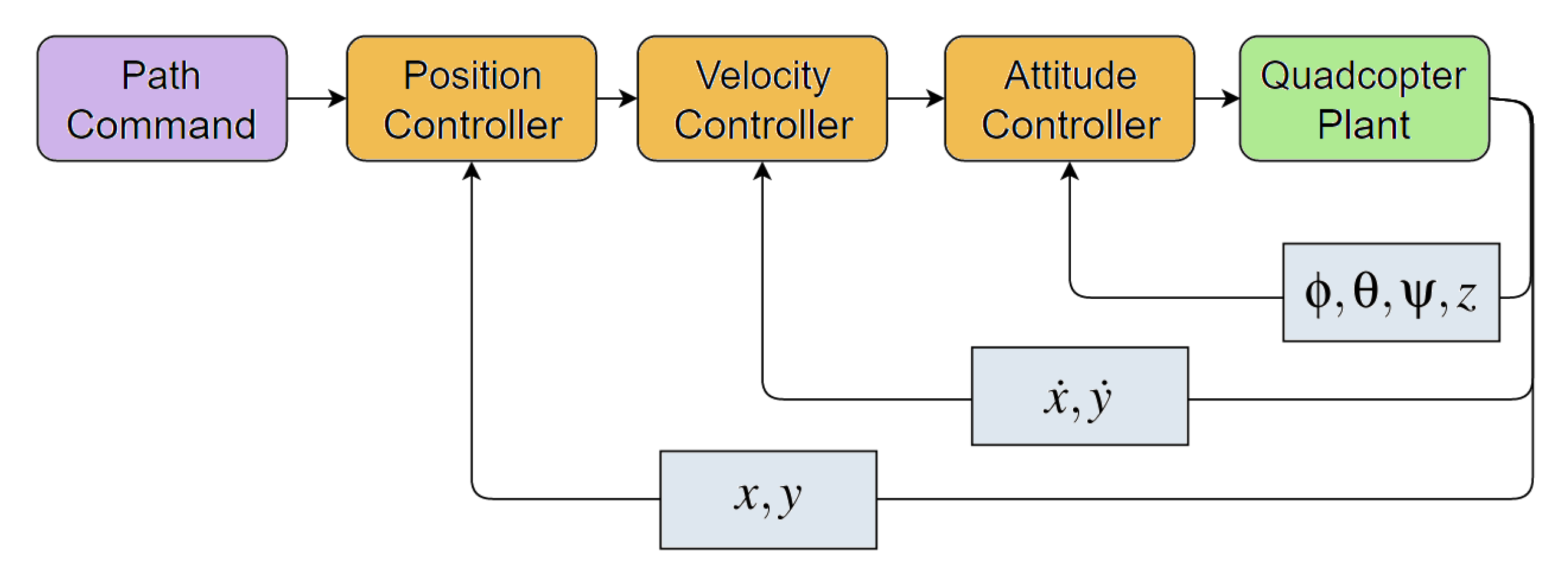
In the case of the first quadcopter control system, a PID cascade architecture has been used to obtain control of the robot. Cascade loops benefit from dividing the control problem into several parts, adding complexity to the overall system but simplifying the individual nested loops. Figure 9 illustrates the control architecture used in this work for the quadcopter. The implemented architecture features three nested PID feedback loops, each one controlling the position, velocity and attitude of the quadcopter respectively.

This controller architecture is set up to track the position of the Strider V1.0 and it is fed from the workspace a yaw and altitude command and a configuration set of parameters for the VTOL algorithm to work. The controller inputs are listed as follows:

“Alt_cmd” and “Psi_cmd” for altitude and yaw command. For the VTOL algorithm, “AppAlt” and “e” control the approaching hover altitude before landing on the moving platform and the position error threshold between the quadcopter and the landing pad before landing respectively. Finally, “LandingSchedule” and “EnableVTOL” control the time when VTOL is commanded and enables or disables the VTOL controller altogether, as their name suggests. When VTOL is disabled, the quadcopter tracks the commanded altitude through “Alt_cmd”.

5.1.2. Inverse Kinematics Approach

The second implemented controller requires a short description of the control basis of this approach. Using the given definition for $\xi$, and assuming that it coincides with the centre of mass of the quadcopter, and the only forces acting on the system are gravity and the thrust from the rotors the motion of the centre of mass is defined by:

$$m\ddot{\mathit{\Gamma }}=U_1{z}_B-mg{z}_E$$

(14)

where m denotes the mass of the quadcopter, $z_B$ and $z_E$ are the direction of the z axis of the body and inertial frame, and $U_1$ is the sum of the thrusts of all rotors.

Taking $\ddot{\mathit{\Gamma }}$ as the input of the control scheme we need to define the desired orientation of the quadcopter to achieve this input command. This can be done following [33], in order to obtain the transformation matrix corresponding to this desired orientation and thus, the desired pitch and roll angles function also of the commanded yaw angle:

$$\begin{array}{cc}\hfill z_B& =\frac{t}{\parallel t\parallel },t={[\dot{x},\dot{y},\dot{z}+g]}^T\hfill \end{array}$$

(15)

$$\begin{array}{cc}\hfill x_C& ={[cos\psi ,sin\psi ,0]}^T\hfill \end{array}$$

(16)

$$\begin{array}{cc}\hfill y_B& =\frac{z_b\times x_C}{\parallel z_b\times x_C\parallel }\hfill \end{array}$$

(17)

$$\begin{array}{cc}\hfill x_B& =y_B\times z_B\hfill \end{array}$$

(18)

Being $x_C$ the x axis of an intermediate reference frame attached to the quadcopter after the yaw angle rotation. This results in:

$${}^W{R}_B=[x_B{y}_B{z}_B]$$

(19)

Euler angles corresponding to the typical convention ZYX can be easily obtained from this transformation matrix.

Concerning the relationship between the total thrust of the rotors and this desired orientation, it is straightforward to see that:

$$U_1=m\parallel t\parallel$$

(20)

Control Architecture

Now that the basis for the inverted kinematics controller approach has been taken care of we can describe the architecture implemented (see Figure 10). It consists of a high level controller and an attitude level controller. The High level controller receives the path commands and outputs the necessary attitude commands to achieve them.

In order to decouple the motion in the xy plane and the acceleration on the $z_E$ axis (height control), the architecture shown in Figure 11 is proposed. Where the lifting acceleration needed is calculated using a PID controller which input is the desired height. The inputs of the proposed controller are the desired height and yaw angle, and the input accelerations $\dot{x}$ and $\dot{y}$.

The controller outputs the Roll, Pitch and Yaw command as well as the throttle command to the inner attitude control loop of the quadcopter. Attitude control is obtained through simple PID controllers for the Roll, Pitch and Yaw of the quadcopter. The output of these PID controllers, along with the thrust command feeds the control mixer, where the individual commands get translated into the throttle speed for each of the rotors.

Path commands for this controller are, once again, “Alt_cmd” and “Psi_cmd” for altitude and yaw command and “ax” and “ay” for the desired accelerations in the horizontal plane with respect to the inertial frame of reference.

5.2. Vessel Control

The control architecture of the Strider V1.0 is easier to implement than the quadrotor system. The system has two inputs: the rudder angle ${\delta }_r$ and the generated thrust T, compared to the four of the quadrotor. Besides this, only two degrees of freedom of the vessel will be controlled. Two separate PID controllers will command the surge speed u and the heading $\psi$ of the vessel. Figure 12 illustrates a simplified scheme of the control architecture implemented.

A way-point trajectory tracking algorithm was also implemented in the control architecture of the Strider V1.0 in order to perform planned sweeps and other autonomous path following tasks. Way-points are defined in Cartesian coordinates $(x_k,y_k,z_k)$ for $k=1,2,\cdots ,n.$ and represent an ordered database of points in the working space. This way-point databases can be expressed as [25]:

$$wpt.pos=(x_0,y_0,z_0),(x_1,y_1,z_1),\cdots ,(x_n,y_n,z_n)$$

(21)

For the implementation of path control based on way-point trajectory planing Line Of Sight(LOS) guidance was used. Once the vehicle has reached the way-point the next way-point is selected. For this purpose, the concept of circle of acceptance is adopted. When the vehicle resides within the borders of a circle of radius ${\rho }_0[m]$ the next way-point in the database is selected. Figure 13 shows the Simulink block architecture used for the controllers and implemented algorithms.

6. Simulation Cases and Performance

This sections covers the experiments made to evaluate the simulation and controllers performance. These simulations showcase its ability to become a basis for development of controllers for researchers and implementation of V-REP and MATLAB’s existing features and tools. It also delves into its utilization and the configuration of the used software. Trajectory tracking for the quadcopter using the cascaded PID and the waypoint guidance controller for the Strider are tested and finally VTOL (Vertical Take Off and Landing) of the quadcopter over the moving USV landing pad is evaluated.

To start using this simulation strategy first a V-REP scene with the provided models of the UAV and USV and the Simulink model needs to be opened. This initializes Matlab’s workspace with the minimum required data so the simulation can run. The demos included with the Simulator present with some examples scenarios of its use.

The outputs of the simulation can be read from the “simout” (or “out”) workspace variables that Simulink creates after finishing a simulation. The logged signals have to be marked using Simulinks data logger. The attached Simulink model logs by default the output vector of the remote API script, following the structure in Equation (11).

The simulation step in both programs and in the remote API interface script is set up to 100 Hz. Although 100 Hz refresh rate on the control loop of the quadcopter may be small for some applications it was selected as it was a middle ground between a high enough frequency rate for controller deployment and small enough so simulation times would not be extremely high.

The Vortex physics engine is used since ODE and Bullet physics engines cannot deal with the three degrees of freedom setup rig for the vessel since the masses of the rig are too small in relation to the mass of the vessel. Also, Vortex provides additional simulation precision and the increased reliability in the interaction between shapes over ODE and Bullet.

Thanks to the use of a physics engine, contact forces and collisions between the simulated robotic platforms do produce disturbances in both platforms. This would allow for disturbance rejection studies and a more realistic behaviour of the platforms.

6.1. Trajectory Tracking

This test showcases the tracking performance of the UAV and the waypoint guidance algorithm for the UAV in action. Two scenarios, for a boxlike path and a sweep mission, have been implemented. These scenarios could be accurate representations of what a research vessel could encounter during a mission.

During this mission the vessel is set to follow a planned path described by a set of waypoints, while the UAV is tasked with tracking and hovering continuously over the position of the vessel. During this missions it is assumed that the drone has complete awareness of the location of the vessel’s landing platform.

These two scenarios correspond to the demo 1 and 2 included in the simulator files. The plots shown in Figure 14 represent the path taken by both the vessel (solid line) and the quadcopter (dotted line) along with the representation of the programmed waypoints for both performed tests. Starting both at the origin and moving clockwise in the case of the box like pattern. The main reasons for the overshoots between closeby way-points seen in the tests are the constant speed and the maximum rudder angle limit the maximum turning angle of the vessel.

Figure 15 illustrates the tracking error of the quadcopter with respect to the Strider V1.0 is very good in straight line passages and has a quick settling time when the Strider V1.0 changes direction.

6.2. Vertical Take of and Landing over a Moving Platform

In this test the implemented VTOL algorithm is used to perform an autonomous VTOL flight. The maximum error threshold between the position of the quadcopter and the centre of the Strider V1.0 landing pad was set to $e=0.1$ m and the approaching altitude before landing 65 cm above the landing pad.

As in the previous simulation case, it is assumed that the drone has complete awareness of the location of the vessel’s landing platform.

The results of the performance of the VTOL tests are shown in Figure 16. It can be seen that the designed algorithm functions properly and that the quadcopter is able to safely land in the platform within the error constrains that were set. In the plots, the three stages of the controller can be easily identified and are separated in different areas. Also a small dip in altitude can be seen around the seventh second, corresponding to a starting “Landing” phase due to the tracking error going below the programmed threshold, however the landing gets quickly aborted and approaching altitude re-established once the tracking error spikes again.

Figure 17 shows a short ghost sequence of a VTOL manoeuvre in the V-REP environment where another successful VTOL operation over a moving platform is attained.

6.3. Simulation Performance

Simulation performance has been evaluated by comparing simulated time vs elapsed time for the simulation. To do this a series of simulations have been performed to obtain a small data pool to make an assessment on performance. The tests were performed on a Windows 10 (x64) machine with an AMD Phenom II X4 965 (3.4 GHz) processor, 8 Gb of RAM and an AMD Radeon HD7700 graphics card.

For data collection, the timing meta-data from the simulation output file and the Simulink profiler were used. On the V-REP side, profiling timings for the tests were not logged since it introduced significant overheads. However simulation pass execution time was measured (for the tests performed on “Lake Scene”) and yielded 1 ms while there was no collision between shapes was detected up to 9ms after the quadcopter lands on the vessel deck. The tests and elapsed times were obtained using the threaded rendering option in V-REP, which speeds up simulation speed.

Figure 18 shows the results of the performed measurements. To obtain a fair comparison, all simulations recreate the same scenario setup in “demo1”, log the output of the simulation and run in normal simulation mode. For each different simulation the tests were performed twice and are, in order: a short 15 s simulation with VTOL disabled (Test 1-2), a longer 35 s simulation with VTOL disabled (Test 3-4) and finally another 35 s simulation with contact between the platforms are performed, VTOL enabled and scheduled to land after 5 s (Test 5-6).

Real time factors (R), across the performed tests show values in the range of [0.5–0.7] depending on the length of simulation, increasing the longer the simulations goes. Since the initialization and termination phases of all the performed tests present very similar time values, the profiler simulation phase time and the elapsed execution time (from the timing meta-data) were used for real time factor calculation.

It is important to note the difference between the elapsed time during simulation recorded by Simulink and the recorded simulation time by the profiler, which is very similar in both iterations of the tests. This difference is due to the introduced external API lag, needed for data transmissions which is proportional to the number of simulation steps performed, and the processing time for each step needed by the physics engine in V-REP which depends on the complexity of the simulation scenario.

Tests 3-4 and 4-6 demonstrate this as a ten second difference between both experiments can be observed. This is due to the added computation time needed by the physics engine once the quadcopter lands on the vessel deck.

The figure showcases the main drawbacks of using an external API based on TCP connections is the additional overhead due to the time it takes the connection to transfer the data. Although ping times between the client and the server were not extremely high (averaging 4 ms), the need for a synchronous operation forces the simulation to transfer data each simulation step. e.g., for each 5 s of simulation, 2 s of processing time (considering a 4 ms average) are “wasted” in waiting for the data connections. It is easy to see from the figures how the actual simulation time recorded by Simulink’s profiler actually renders values of $R\ge 1$, being the API overhead one of the bigger factors in the reduction of the real time factor.

Simulation time consistency is within 2 to 3 s, probably due to the random seed initialization in physics engines and CPU maximum usage bottlenecks.

7. Conclusions

This work presents a simulation strategy for a multi-robot collaboration scheme between a UAV and a USV. Although its initial motivation was the development of a prototyping platform for deployment of control architectures for both the UAV and USV in limnology related surveys, the strategy proposed in this paper also allows testing and developing both autonomous vehicles independently. Thanks to the modularity provided by Simulink models and the independent control of robotic models in V-REP the simulation strategy is highly flexible and customizable.

The dynamic modelling of both platforms provide a suitable scenario for testing and validation of coordinated behaviours between aerial and maritime platforms. An initial control strategy design can be obtained as the results from this work portray. However the lack of heave and roll dynamics on the surface vessel models provided could lead to differences in behaviour between the simulated and real platforms in scenarios where those dynamics are relevant. Nonetheless, inclusion of the missing degrees of freedom on the USV platform and other exogenous effects not considered in this work could be easily included thanks to the ease of implementation robotic simulators such as V-REP provide.

This can be seen in works such as [34] or [18] where simple simulation environments implemented using V-REP have been successfully used. In these and similar works the simulated response of the system yielded very comparable responses in the real experiments. This performance is only dependent on the correct modelling parameters of the robotic plants used, and the requirements for simulation fidelity.

The used software (Matlab and V-REP) provides great compatibility and portability among different OS and platforms and does not require additional software to be run. V-REP allows the inclusion of realistic sensors and camera feeds which support visual processing algorithms, expanding the scope of the work to be done within the environment and thanks to the popularity of both platforms there exist a great availability of pluggins and addons that can expand the extension of tasks to be achieved.

V-REP’s selection over a Gazebo based implementation provides a more robust execution, a wider set of features by default and a more intuitive use. Besides this, unlike Gazebo, it has the ability to directly import CAD models and includes mesh manipulation tools that allow for quick modelling of usable and efficient robot models among other various key features over Gazebo.

Thanks to this, the simulation strategy provides a quick way for prototyping of control strategies for collaborative or individual operation and the study of the interaction between the different robotic platforms and the environment.

Some of the future improvements to the simulation environment are an increase in simulation speed performance and the inclusion of more features such as more detailed hydrodynamic model of the Strider V1.0 including a six degrees of freedom model, more complex control architectures and ROS integration. Other improvements to be considered are the addition of a friendly GUI, a model library with different robots and support for control of multiple copies of the same robot.

But since this is a project that aims to be open-source and available we are looking forward to the community to contribute with advanced control architectures and robot models libraries to improve the usability and utility of this prototyping platform. This project along with video resources (goo.gl/hRC5GM) of the simulations is available at the github repository (github.com/OmarVelascoAnrar/UAV_USV_Simulator).