1. Introduction
Eutrophication and water pollution in rivers caused by non-point pollution sources have recently become a serious worldwide problem [
1,
2,
3]. Particularly, in agricultural areas, several pollutants such as high-nutrient composts and waste materials containing large amounts of nitrogen and phosphorus readily flow into nearby rivers via surface runoff, which leads to eutrophication and algal blooms [
4,
5,
6,
7]. River contamination not only affects aquatic ecosystems but also urban residents who depend on these water bodies as drinking water sources [
8]. Therefore, non-point pollution management is critical to minimize water pollution. The large-scale development of agricultural areas into farmlands in South Korea has resulted in an increased demand for fertilizers and pesticides. Due to the occurrence of torrential rains in the summer season (i.e., from June to August) [
9], water pollution caused by non-point sources is becoming a serious problem [
10]. Non-point sources of water pollution are of particular concern in agricultural areas, as these regions lack the degree of management and oversight of urban areas where water supply and sewage infrastructure are relatively well established.
Among the many non-point pollution sources, outdoor compost piles (OCPs) are becoming a serious problem in agricultural areas in South Korea. Given that compost contains large amounts of nitrogen and phosphorus, it is used to increase the growth of crops by supplying nutrients to the soil. However, excessive compost use is a major cause of eutrophication, as these nutrient-rich materials often reach nearby rivers due to surface runoff [
11,
12]. Compost is mainly applied outdoors in agricultural areas in South Korea, thus raising concerns about water pollution [
13]. Therefore, central and local government officials must conduct regular OCP site monitoring and conduct a thorough assessment of OCP pollution to improve OCP management strategies. However, there are severe limitations regarding the human labor, cost, and time required to conduct a full OCP survey in large areas, thus highlighting the need for more efficient OCP monitoring and management tools.
Many studies have explored the use of images captured from unmanned aerial vehicles (UAVs) and satellites to efficiently characterize specific objects on the earth’s surface. Particularly, UAVs are being used in various fields [
14,
15,
16,
17,
18] because they can easily acquire high-resolution (i.e., centimeter-level resolution) images as well as various spectral images, while flying at low altitudes [
19]. UAVs are highly useful for categorizing or detecting specific objects via object-based supervised and unsupervised classification [
20,
21,
22,
23,
24,
25]. Additionally, technologies for more accurate object detection have been recently developed by applying various machine learning and deep learning techniques, such as support vector machines (SVM), random forest (RF), decision tree (DT), and k-NN [
26,
27,
28,
29,
30,
31,
32,
33]. Nonetheless, a technology for OCP detection using UAV images coupled with machine learning techniques has not yet been developed.
Therefore, our study sought to develop a machine learning technique to efficiently detect OCP using UAV images and various machine learning techniques in targeted areas of Samga-myeon, Hapcheon-gun, where large-scale agricultural lands with a high occurrence of OCPs have been established. To achieve this, (i) RGB, multispectral image, and thermal infrared imaging data were acquired in August and October 2019 using UAVs, (ii) vegetation index images were analyzed using multispectral imaging, (iii) OCPs were classified and spectral characteristics were analyzed, and finally, (iv) the OCP classification accuracy of various machine learning techniques was compared.
2. Materials and Methods
2.1. Study Area
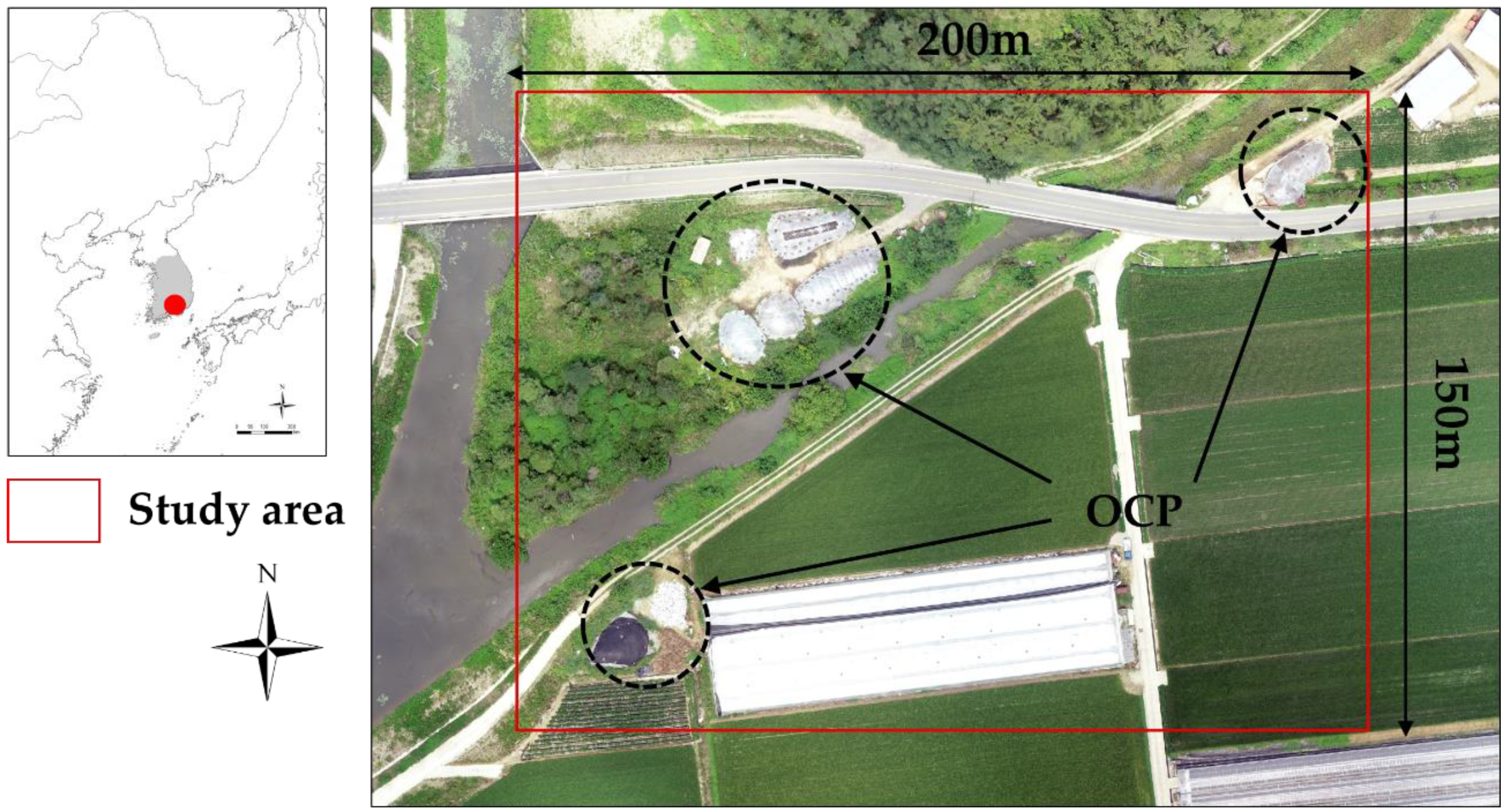
This study was conducted in areas known for the occurrence of OCPs (35°24′48″ N, 128°6′17″ E) in the region of Samga-myeon, Hapcheon-gun, located in the south of South Korea (
Figure 1). The study area was 200 m in width and 150 m in length. The OCPs distributed in the study area were located in an area near the river, where cropland and greenhouses were also located. On cultivated land, rice is grown from June to October, whereas field crops are grown from November to May. During the rice cultivation period, the OCPs are stacked around the cultivated area and covered with plastic, after which they are scattered on the cultivated land once the harvest ends in November.
Korea exhibits four distinct seasons, with rain and torrential rain events occurring primarily during the summer period (i.e., from June to August). Therefore, if OCPs are not properly managed, they may be washed away by the rainfall and flow into nearby rivers. Therefore, it is necessary to effectively investigate and manage OCPs to proactively prevent water pollution.
2.2. Production of UAV Orthoimages and Vegetation Indices
In this study, RGB, multispectral, and thermal infrared images were collected from UAVs. The images were taken in August and October 2019 when the weather conditions allowed for UAV operation. Images were acquired from 11 am to 2 pm, when the sun’s altitude was highest. RGB and thermal infrared images were obtained by mounting both a Zenmuse X3 camera and a FLIR Vue pro R infrared camera (spectral band: 7.5–13.5 μm, accuracy: ±5 °C, emissivity: 0.98) on a DJI Inspire 1 UAV, respectively. For multispectral images, image data for five spectral bands (blue, green, red, NIR, and red-edge) were acquired by mounting a Red Edge-M multispectral camera on a 3DR-solo UAV.
Table 1 details the equipment used for UAV photography.
The flight path employed for each UAV imaging method was established based on the range of the study area, and Inspire 1 and 3DR-solo UAVs were alternately operated. The image acquisition altitude was set to 150 m, and the image overlap was set to 85%. The UAV images were collected as orthoimages using the Pix4D Mapper software. The final orthoimages were obtained by submitting the multispectral images and the thermal infrared images to geometric correction based on the RGB images.
Various vegetation indices were analyzed to understand the spectral characteristics of OCP using five spectral images taken with a multispectral camera. Four vegetation indices, including the widely-used normalized difference vegetation index (NDVI), the enhanced normalized difference vegetation index (ENDVI), the normalized difference RedEdge index (NDRE), and the green NDVI (GNDVI) were used. The formulas for these vegetation indices are summarized in
Table 2.
2.3. OCP Boundary Division and Spectral Characteristic Analysis
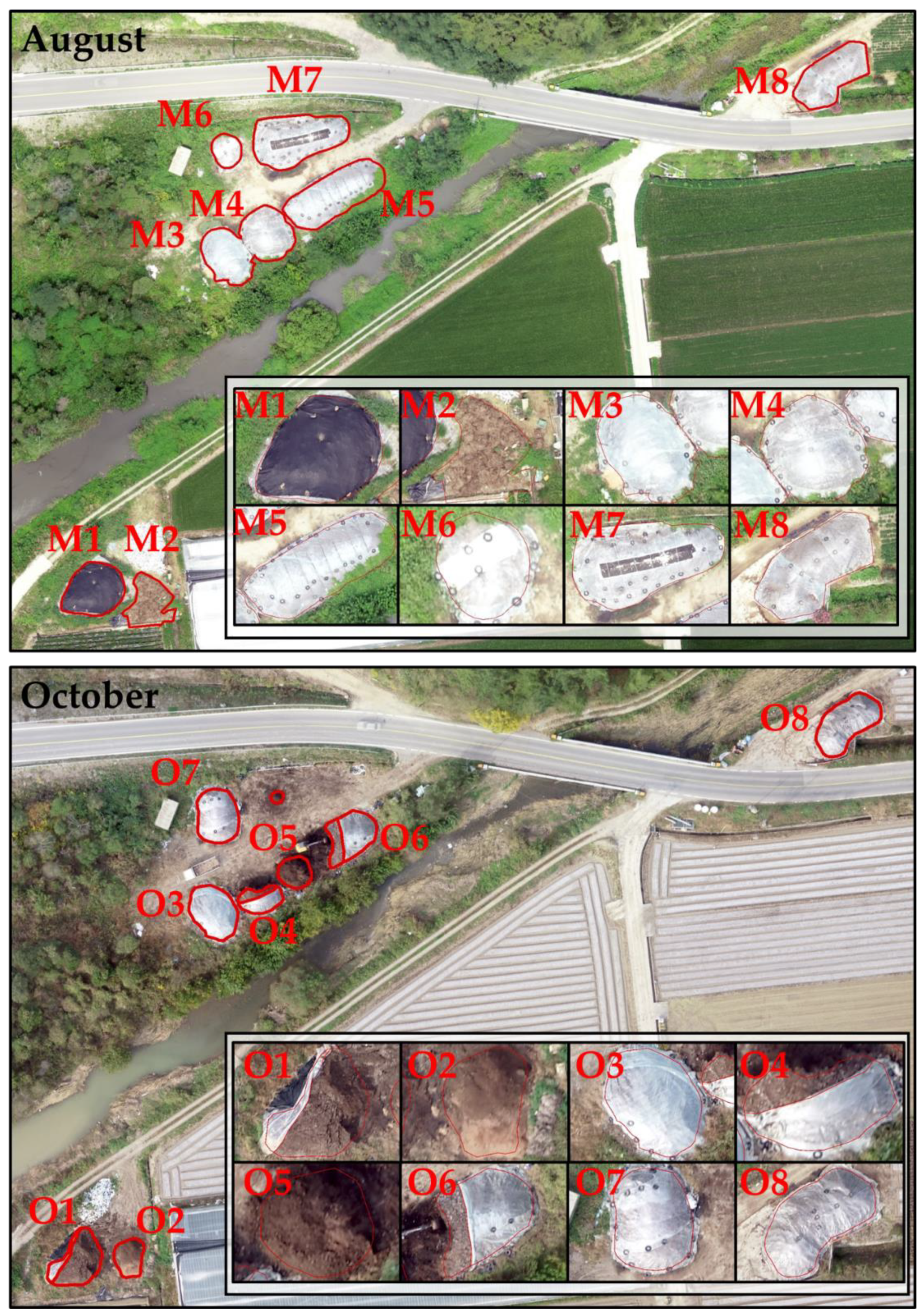
The boundary of OCPs were separated through vectorizing using RGB images and the ArcGIS 10.2 programs (
Figure 2). Moreover, to account for current OCP management practices, polygons were divided into those that were covered with plastic (vinyl) and those that were not. Therefore, OCPs were classified into three types: OCP, plastic-covered OCP, and others.
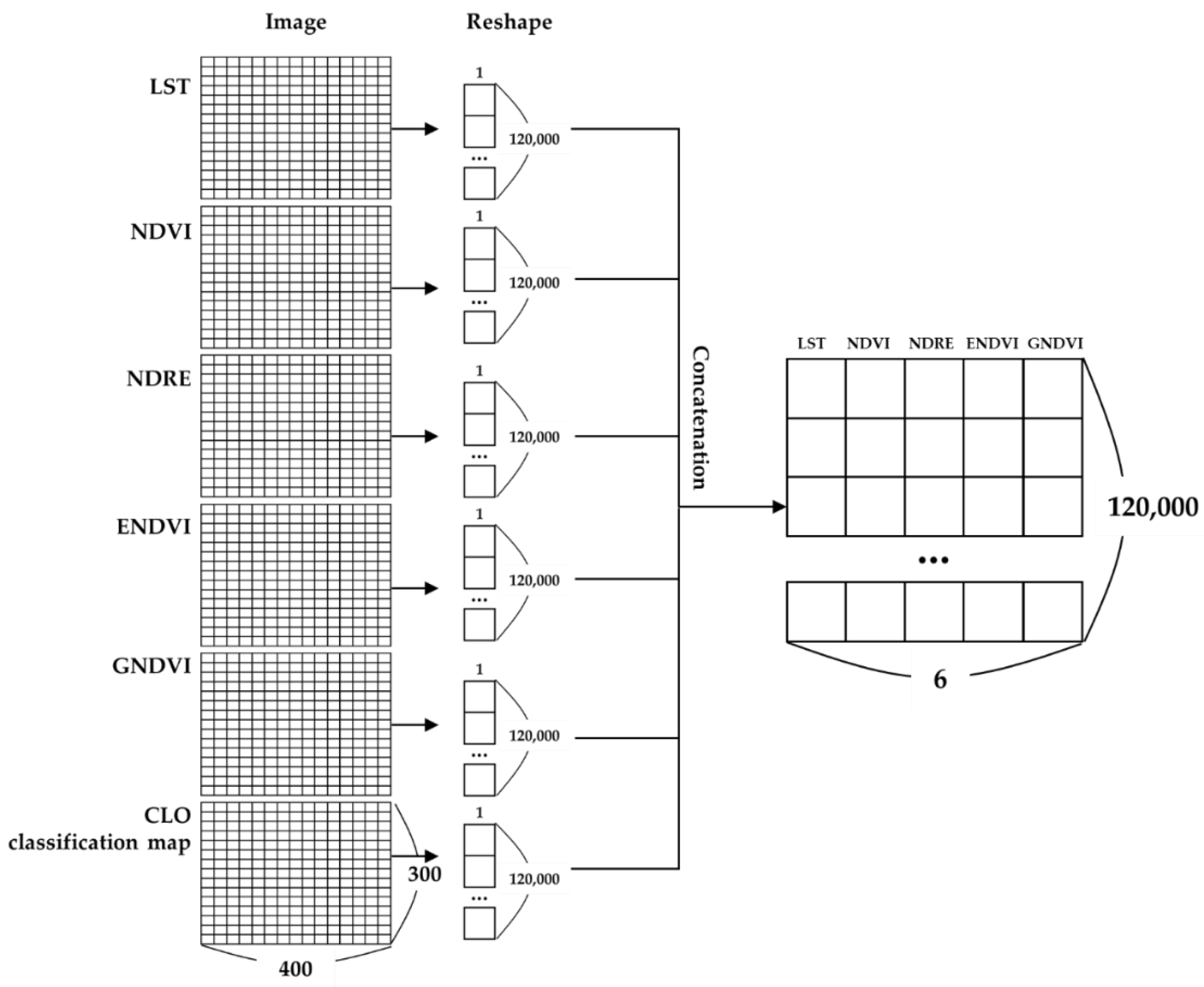
Four vegetation index images produced from multispectral images and surface temperature extracted from thermal infrared images were used to understand the spectral characteristics of OCPs. First, due to the differences in spatial resolution between the data associated with each of the acquired images, all images were adjusted to the spatial resolution of the surface temperature image with the lowest resolution (50 cm × 50 cm). OCP classification data were also set to the same spatial resolution (50 cm × 50 cm), and polygon vector data were converted into raster data. All image data (400 × 300 pixels) were resized to the boundary of the study area and the data for each image (four vegetation indices, surface temperature, OCP classification data) were reshaped to one column (1 × 12,000) using Python 3.7. A database was constructed by concatenating each column, and the characteristics of the vegetation index and surface temperature were analyzed according to the classified OCP type (
Figure 3).
2.4. Prediction of OCP Classification Using Machine Learning
Using the database shown in
Figure 4, the accuracy of the OCP classification prediction was compared among various machine learning techniques, including SVM, decision tree (DT), random forest (RF), and k-NN using the ski-learn package in Python 3.7. The training data to test data ratio was 60% to 40%, and the data were randomly selected.
Regarding the SVM analysis, we also compared the performances between linear SVM and nonlinear SVM, and their accuracy was compared by adjusting the C parameter from 10−4 to 108. The C parameter establishes how many data samples are allowed to be placed in different classes. The smaller the C parameter, the higher the likelihood of outliers, creating a general decision boundary. In contrast, a larger C parameter results in a lower likelihood of outliers, which favors the identification of the decision boundary. The accuracy of the DT analysis was assessed by adjusting the maximum depth and random state values from 0 to 10 and 0 to 100, respectively. Max depth is a parameter representing the maximum depth of a tree to train a model. However, overfitting may occur as the depth increases. Therefore, an appropriate maximum depth setting is required for accurate model prediction. A random state is used to divide the data by finding values of elements that can accurately explain the data classification at the time of decision tree division. The RF adjusted n estimator and random state values, in which the n estimator is a variable that adjusts the number of trees to be created, were set from 0 to 20. As in the decision tree, the random state is used for dividing the data of the tree, and the accuracy was compared by inputting the highest accuracy value in the n estimator and setting it from 0 to 100. For k-NN, the accuracy was compared by setting n neighbors from 0 to 10. The n neighbor is a variable that determines the number of similar data used to predict results. When the number of n neighbors increases, the degree of similarity of the data selected as similar data increases. Therefore, it is necessary to set appropriate n neighbors because the classification range is narrow and classification errors occur.
As described above, accuracy was compared by adjusting the four machine learning techniques and variables, after which the machine learning technique with the highest accuracy and the corresponding variable values were obtained. The OCP classification prediction results were then analyzed based on the derived model, after which its applicability and accuracy for field OCP were evaluated.
3. Results
3.1. Spectral Characteristics by OCP Type
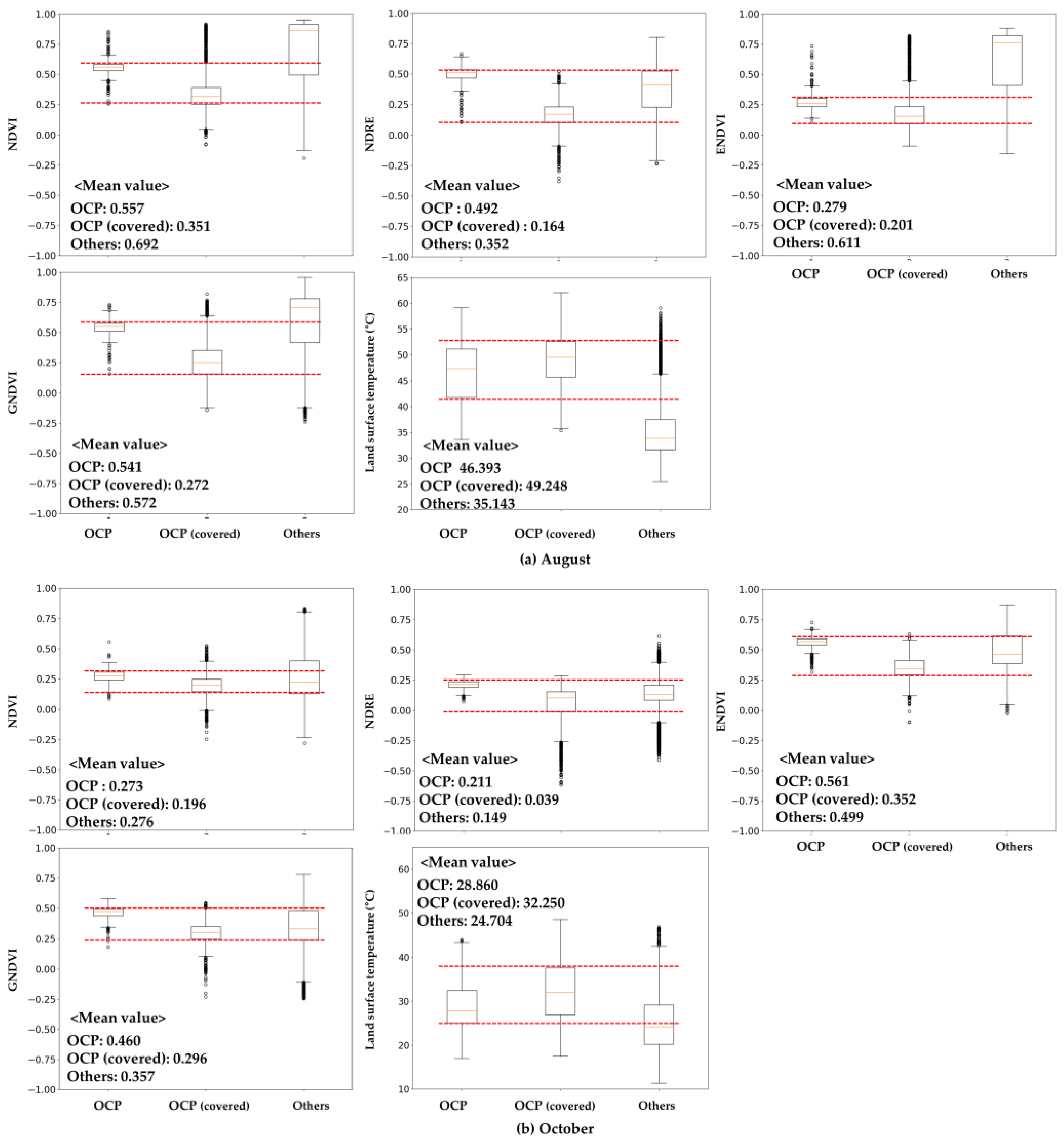
Figure 4 shows the results of analyzing the characteristics of various vegetation indices using the OCP classification type. In August, the number of uncovered OCPs was higher than the covered OCPs according to all vegetation index values assessed herein. Particularly, the difference between the average value of OCPs and covered OCPs according to the NDRE was 0.328, followed by the GNDVI (0.269) and NDVI (0.206). The ENDVI was 0.078, and the difference between OCPs and covered OCPs was negligible. However, the difference in the vegetation index from other types was largest, and it did not overlap with other types, even within the 25–75% range of the boxplot. The NDVI, NDRE, and GNDVI, OCP overlapped with some of the other types. The surface temperature was 2.855 °C lower in OCPs (46.393 °C) than in covered OCPs (49.248 °C). The difference in surface temperature from other types was also very large at approximately 10 °C. In October, the difference between the vegetation index and the surface temperature by type was lower than that of August, but the vegetation indices of OCPs and covered OCPs did not overlap within the 25–75% range of the boxplot. As observed in August, the vegetation indexes for OCPs were slightly higher than that of covered OCPs. The surface temperature was lower in OCPs (28.860 °C) than in covered OCPs (32.250 °C). Upon comparing the characteristics of various vegetation indices and surface temperature according to the OCP type by period, the vegetation indices were clearly classified according to whether the OCP was wrapped in plastic, and the GNDVI was the most distinct among them in August compared to October. However, other types were not clearly distinguished from OCPs except for the ENDVI and surface temperature in August.
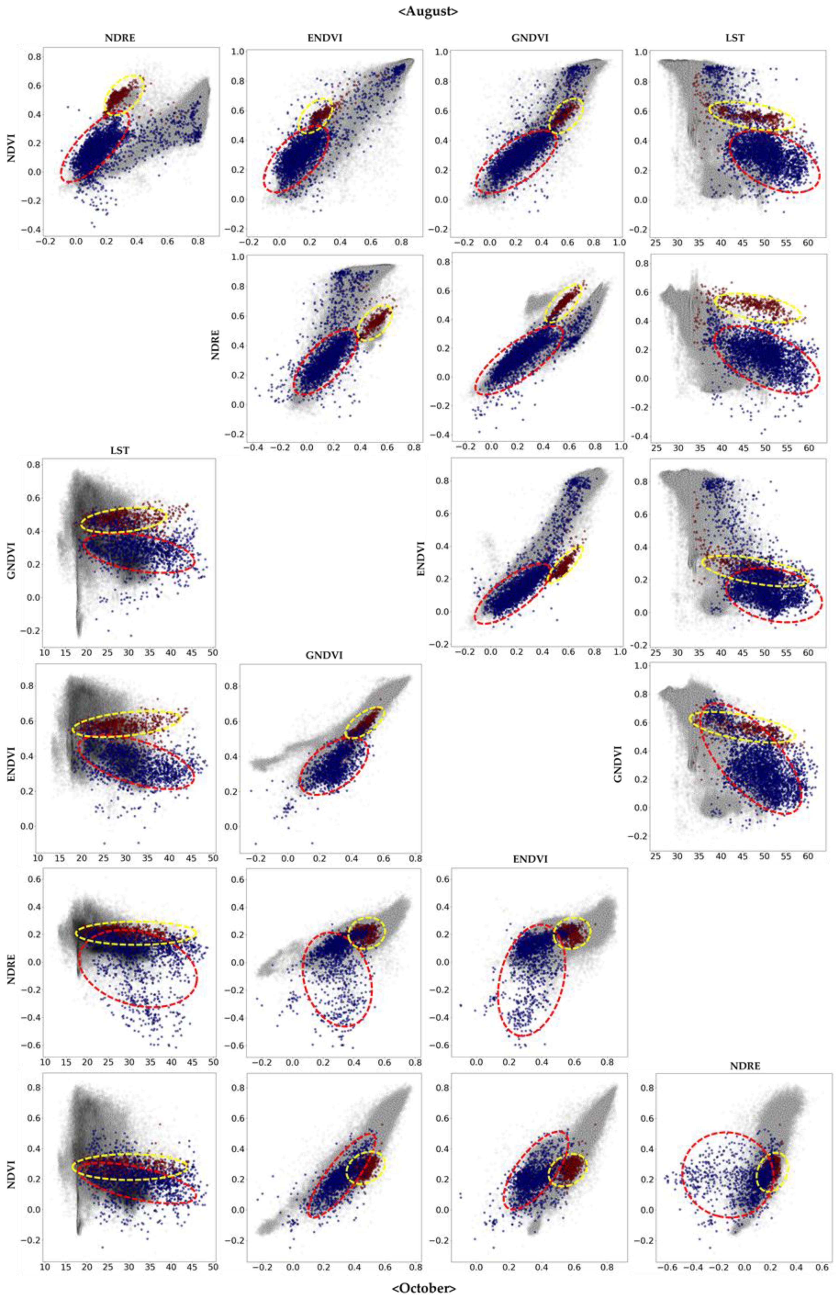
Figure 5 shows the results of scatterplot analysis comparing various vegetation indices and surface temperatures by period. Upon comparing the August vegetation indices, it was confirmed that the distributions of OCPs (red dotted line) and covered OCPs (yellow dotted line) were clearly distinguishable. However, when comparing the surface temperature and vegetation indices, OCPs and covered OCPs were classified only in the NDRE, and not in the remaining vegetation indices. When comparing the vegetation indices in October, OCPs and covered OCPs were divided between the NDRE and GNDVI, NDRE and ENDVI, and GNDVI and ENDVI, and the surface temperature was clearly divided into the ENDVI and GNDVI groups. Therefore, the GNDVI and ENDVI are useful for OCP classification in October.
After analyzing the characteristics of various vegetation indices and surface temperatures according to the OCP type through boxplot and scatter plot analyses, we found that the types of vegetation indices that can classify OCP types varied. In August, for example, all vegetation indices could be classified into OCP and covered OCP types, but vegetation index values overlapped with other types. The same phenomenon occurred in October. In contrast, it was difficult to clearly classify the OCP type, as demonstrated by the scatterplot results. Nonetheless, we confirmed that the OCP type could be distinguished when compared with certain vegetation indices. Therefore, because the classification characteristics of OCPs may vary depending on which data is used for vegetation indices and surface temperature, various vegetation indices and surface temperatures were applied as variables to classify OCP types using machine learning, thus rendering more accurate classification results.
3.2. Comparison of Machine Learning Accuracy
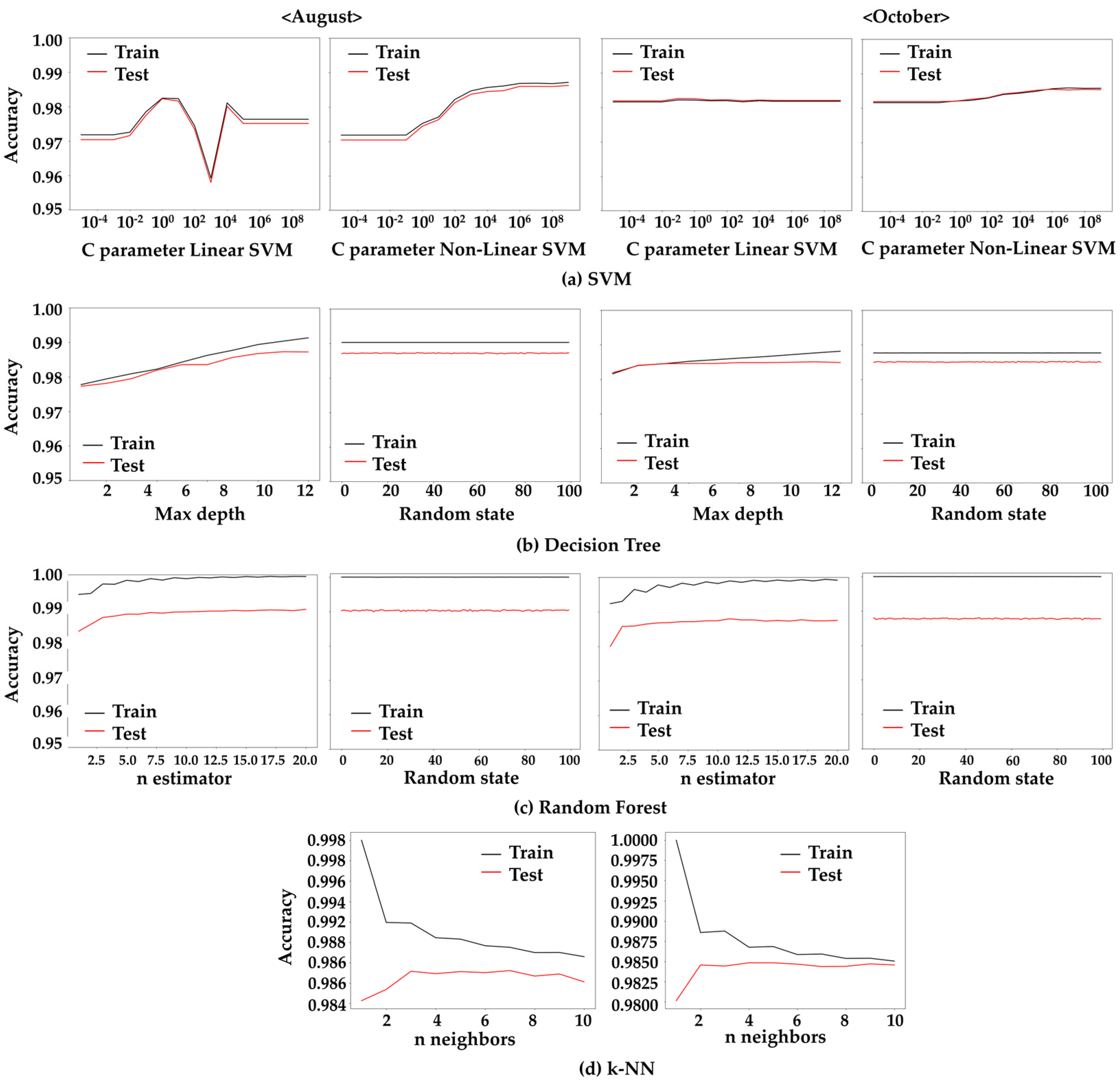
Figure 6 shows the results of the comparison of accuracy by adjusting various machine learning techniques and variables for OCP classification. In the August linear SVM, when the C parameter was 10
3, the accuracy was lowest at 0.96, and when the C parameter was 10
0, the best accuracy was 0.982. Moreover, the accuracy of the non-linear SVM increased as the C parameter increased, and then remained constant starting from 10
4. In the October linear SVM, the accuracy remained constant at approximately 0.98, even if the C parameter changed. In the non-linear SVM, as in August, the accuracy increased as the C parameter increased, but the difference was not significant. The non-linear SVM had a slightly higher accuracy than the linear SVM, and when the C parameter was 10
10, the highest accuracy was 0.986 in August and 0.985 in October.
Upon comparing the accuracy by adjusting the maximum depth and random state of the decision tree, the maximum depth was set from 1 to 10, whereas the random state was set from 0 to 100 by inputting the highest accuracy value in the maximum depth to compare the accuracy. As the maximum depth value increased, the accuracy of the test value increased. When the maximum depth was 8, the highest accuracy was 0.987 in August and 0.985 in October. Even if the value of the random state changed, the accuracy was constant at 0.987 in August and 0.985 in October. Regarding the random forest analysis results, the accuracy of the test value increased as the n estimator value increased, while the accuracy of the test value at 10 was confirmed to be 0.989 in August and 0.987 in October. The random state did not change the accuracy, even when the value increased. Lastly, k-NN’s accuracy decreased as n neighbors increased. The test data exhibited the highest accuracy at 0.987 in August and 0.984 in October when the n neighbor’s value was set to 3.
When the n estimator was set to 10 in the random forest, the accuracy of the OCP classification in August and October was highest. However, when the optimal variable values were implemented in all machine learning techniques, except for the linear SVM, the difference in accuracy was minimal (approximately 0.003). Therefore, we sought to compare the OCP detection results predicted by each machine learning technique to determine the most appropriate technique for OCP detection.
3.3. Comparison of Predicted OCP Detection Results
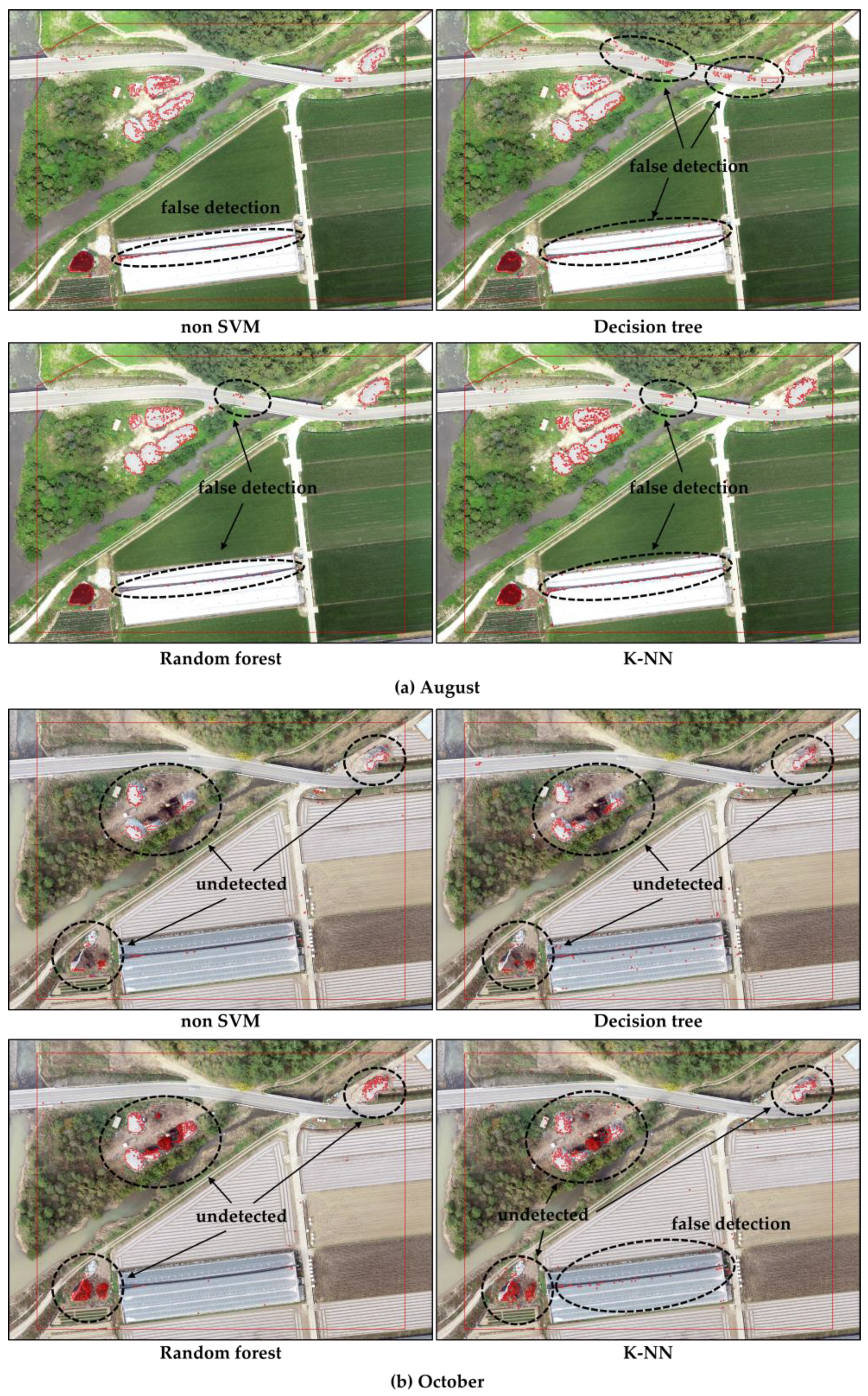
Figure 7 shows the results of classifying OCPs using various machine learning techniques. In August, some greenhouses and spaces between greenhouses and roads were falsely detected as OCPs. The results were identical once all machine learning techniques were applied, albeit with different areas. DT and k-NN had frequent false detections. In October, the spaces between greenhouses or areas where roads were falsely detected as OCPs were fewer than in August; however, the overall OCP detection performance was inferior compared to that of August. Additionally, other falsely detected areas were identified as the upper surface of greenhouses instead of the space between the greenhouses. False detection is believed to be due to vegetation index and surface temperature values similar to those of OCPs.
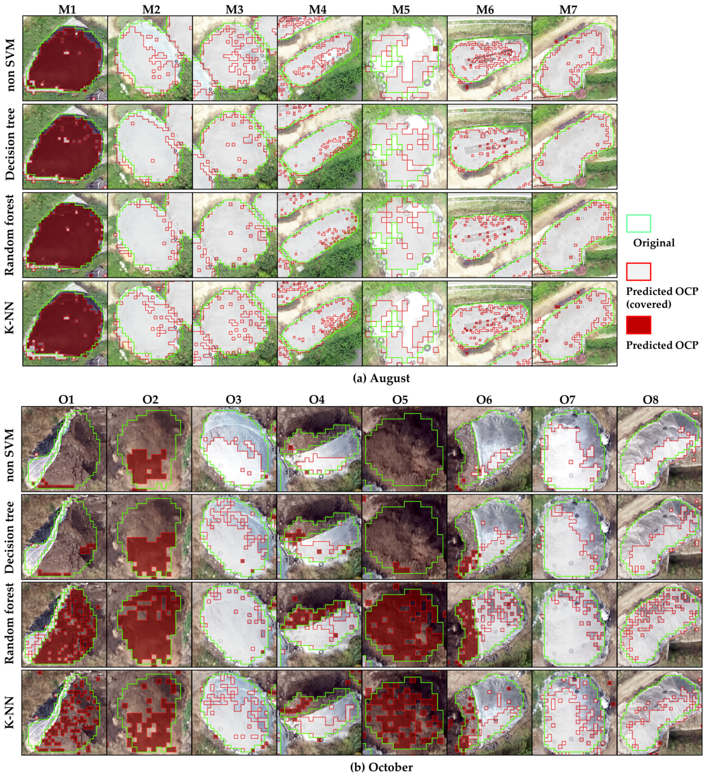
Figure 8 shows the results of different machine learning techniques for OCP detection. In August, OCPs can be found to be well-predicted for all machine learning techniques. However, M5 was not detected compared to original, and in non-linear SVM, the difference between original and predicted OPCs was the greatest. In October, it can be seen that the difference between original and predicted OPCs in all machine learning techniques except RF is large.
Table 3 shows the results of analyzing the difference between the area of the OCP type predicted for each machine learning technique and the area of the original OCP type. In August, OCPs exhibited the smallest difference in area (5.25 m
2) when RT was applied, and the largest difference of 15.75 m
2 in DT. However, when covered OCPs were detected, DT exhibited the smallest area difference of 28.25 m
2, followed by the RF with 49.50 m
2. For the other types, the area difference of DT was 12.50 m
2 and that of RF was 54.75 m
2. It was also confirmed that the non-linear SVM had a very large area difference compared to the other machine learning techniques. This may be the result of false detection of spaces and roads between greenhouses, as illustrated in
Figure 6. Therefore, the DT and RF techniques were very effective for OCP detection, with RF having a particularly good performance.
We also found that the area difference was larger in October than in August when detected by machine learning. When RF was applied, OCPs and covered OCPs exhibited the smallest area differences of 33.75 and 69.75 m2, respectively. Unlike August, the area difference for k-NN was the second lowest (OCPs: 89.00 m2, covered OCPs: 172.00 m2). As mentioned above, there were fewer falsely detected areas in October than in August, but there were many cases where OCPs were not detected, thus resulting in a significant difference in the OCP area. RF was found to be particularly suitable for OCP detection in October, as it rendered the lowest area differences.
Therefore, the most effective method for OCP detection among the various machine learning techniques assessed herein was RF. Moreover, setting the n estimator to 10 produced a predictive model with the highest accuracy. However, although a prediction model with an accuracy of approximately 0.990 was obtained, some areas were falsely detected, and therefore, a strategy to overcome this problem is still needed.
4. Discussion
Our study compared the ability of various machine learning techniques to detect OCPs using UAV images. All machine learning techniques studied herein exceeded a 0.96 accuracy; however, instances of false detection were identified in some areas. This was likely due to variations in the spectral characteristics of OCP regions. For example, as shown in
Figure 8, some OCPs could not be detected due to shadows or because a tire was placed on the vinyl to prevent it from being blown away by the wind. As confirmed by the results in
Figure 4 and
Figure 5, the vegetation indices and the surface temperature varied depending on the type of OCP, which appeared to be the cause of false OCP detection. Therefore, it is judged that it is possible to determine the location of OCPs through the results of this study, but it is judged that there is a limit to analyzing the exact area and boundary of OCPs. If the area and boundary of OCPs can be accurately analyzed, it will be possible to predict the amount of OCPs. As UAV can analyze digital surface models (DSM) through point clouds, it can also analyze volume [
11]. In order to utilize the results of this study more usefully, it is judged that it is necessary to supplement these data and technologies additionally.
Previous studies have also sought to detect specific objects using different machine learning approaches. For instance, Hassanijalilian et al. [
32] compared the DT, RF, and adaptive boosting (AdaBoost) models using image data to detect iron deficiency in soybeans. The results showed that DT, RF, and AdaBoost exhibited precision ranges of 0.54–0.65, 0.66–0.74, and 0.72–0.79, respectively. Feng et al. [
38] attempted urban forest mapping through RF and texture analysis using UAV orthoimages and achieved an accuracy of 73%–90%. Herrero-Huerta et al. [
39] predicted soybean detection and harvesting rates using RF and eXtreme gradient boosting (XGBoost), and the accuracies of RF and XGBoost were 90.72% and 91.36%, respectively. Most previous studies achieved less accurate results than the results obtained herein. Particularly, when the same RF technique was applied, the accuracy of this study was significantly higher. Due to the differences in the characteristics of the study area, the type of image data used, and the type of object to be detected, the accuracy of these studies cannot be directly compared. However, it is considered an achievement that the results of applying the machine learning technologies in this study for the detection of OCPs have higher accuracy than previous studies. In particular, the fact that we were able to know which technology is most effective and how accurate is the level of accuracy for the detection of OCPs will lead to further improvement of the investigation method of OCPs and the use of UAV in the future for the management of non-point pollutants and improvement of water quality. It is judged to be a possible research result.
Several recent studies have recently implemented various machine learning and deep learning techniques for the detection of specific objects, including convolutional neural networks (CNNs) and deep neural networks (DNNs); however, a vast amount of training data is required for accurate object detection [
40,
41]. This study used the pixel values of spectral images captured by drones as training data, and applied various machine learning techniques to derive results with very high accuracy. However, additional input data may be required to improve accuracy and minimize errors or undetected areas. Therefore, the procedures described herein could be utilized for the effective management of OCPs in the future as well as to improve the management of non-point pollution sources and aquatic environments.
5. Conclusions
This study compared the accuracy of different machine learning techniques for the detection of OCPs, which are important non-point pollution sources in agricultural areas of South Korea, using UAV image data. The accuracies of all four machine learning techniques studied herein were found to be very high, exceeding 0.96. In this study, UAV and machine learning techniques were jointly implemented for the efficient detection of OCPs, and extremely promising prediction results were obtained. Importantly, the proposed approach provides an efficient means to predict the location and area of OCPs over a large region of interest based solely on photographs obtained with UAVs, thus eliminating or greatly minimizing the need to conduct inefficient OCP site assessments. Additionally, given that UAV images also provide location information, the predicted results can be effectively utilized for non-point pollution source and water quality management by linking the data with spatial information. However, it is not possible to analyze the uncertainty when applied to other areas because the accuracy of the detection of OCPs was analyzed only in this study area. In the future, it is judged that there is a need to compensate for this uncertainty, and will be conducted to efficiently detect not only OCPs, but also various other difficult-to-detect non-point sources of water pollution using UAV images, machine learning, and deep learning techniques.


