Comparison of Sentinel-2 and UAV Multispectral Data for Use in Precision Agriculture: An Application from Northern Greece
Abstract
1. Introduction
2. Materials and Methods
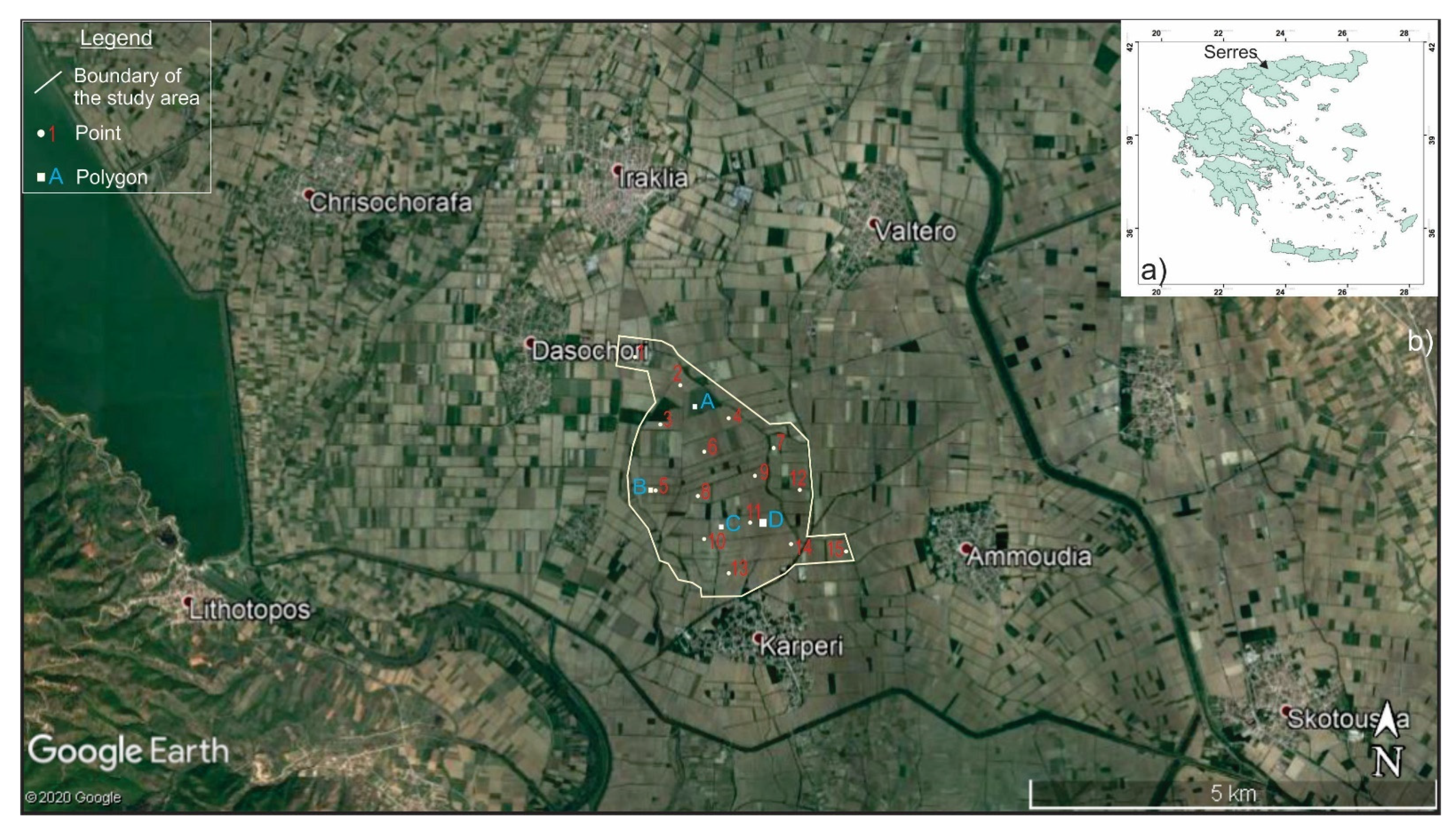
2.1. Study Area
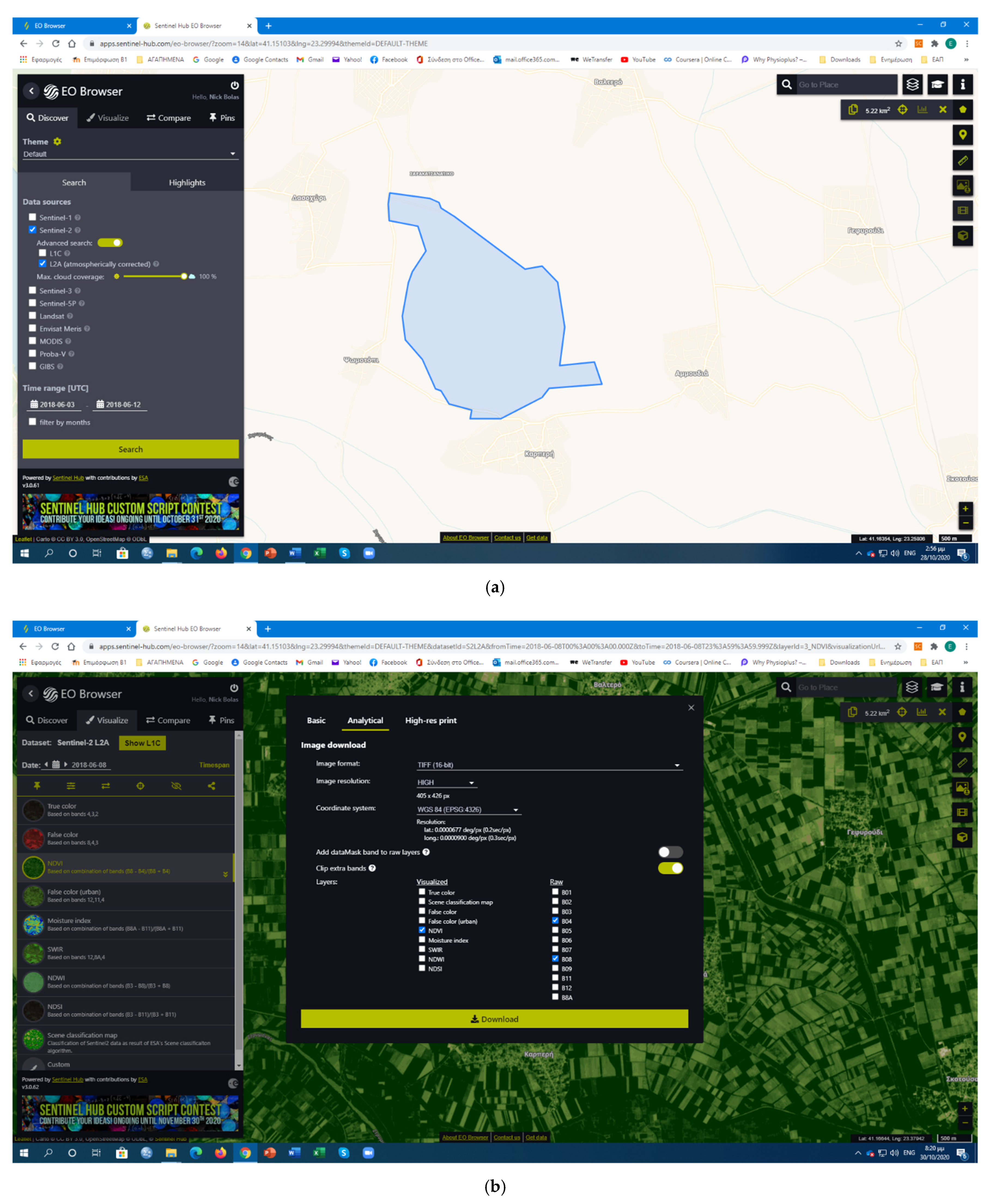
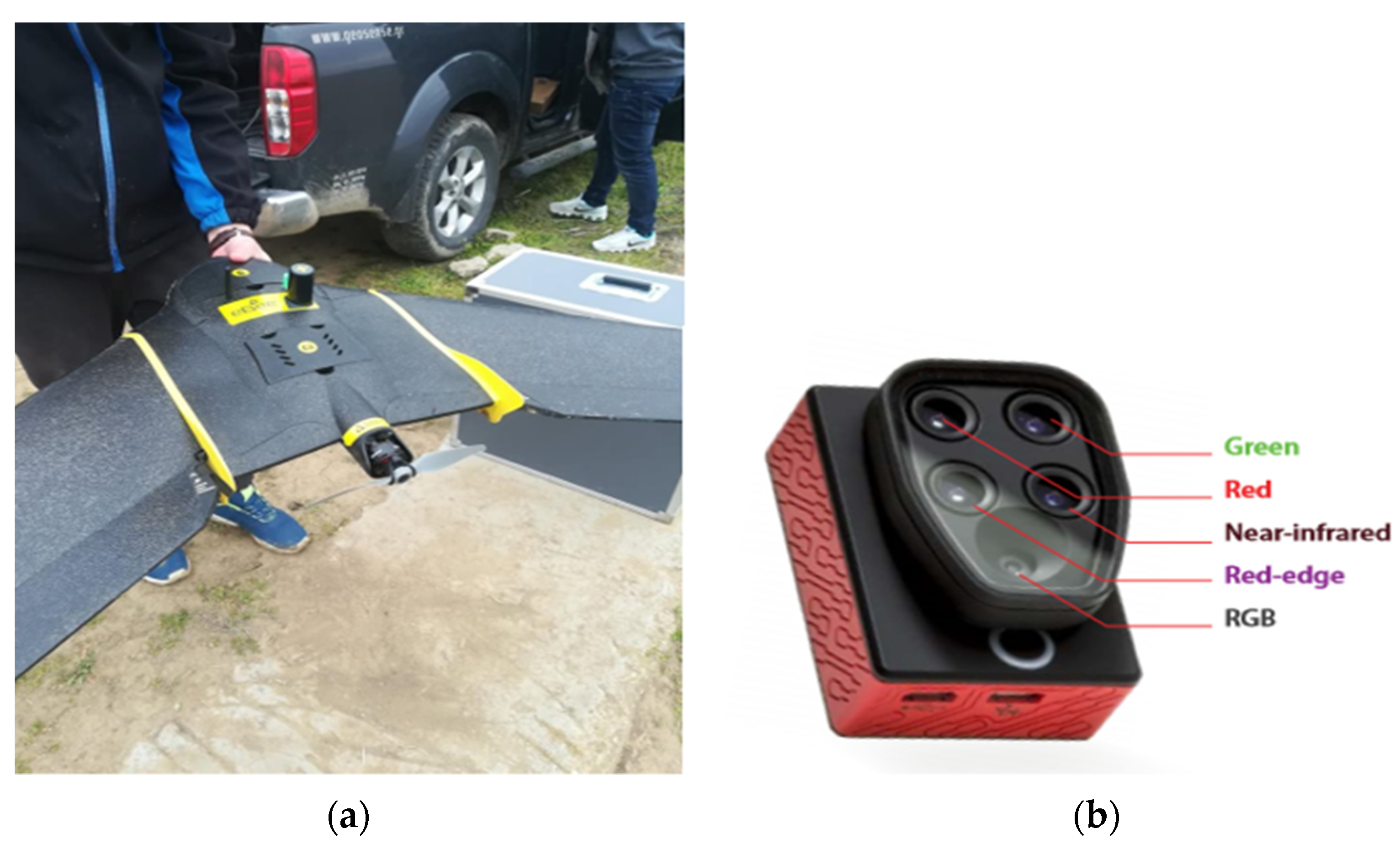
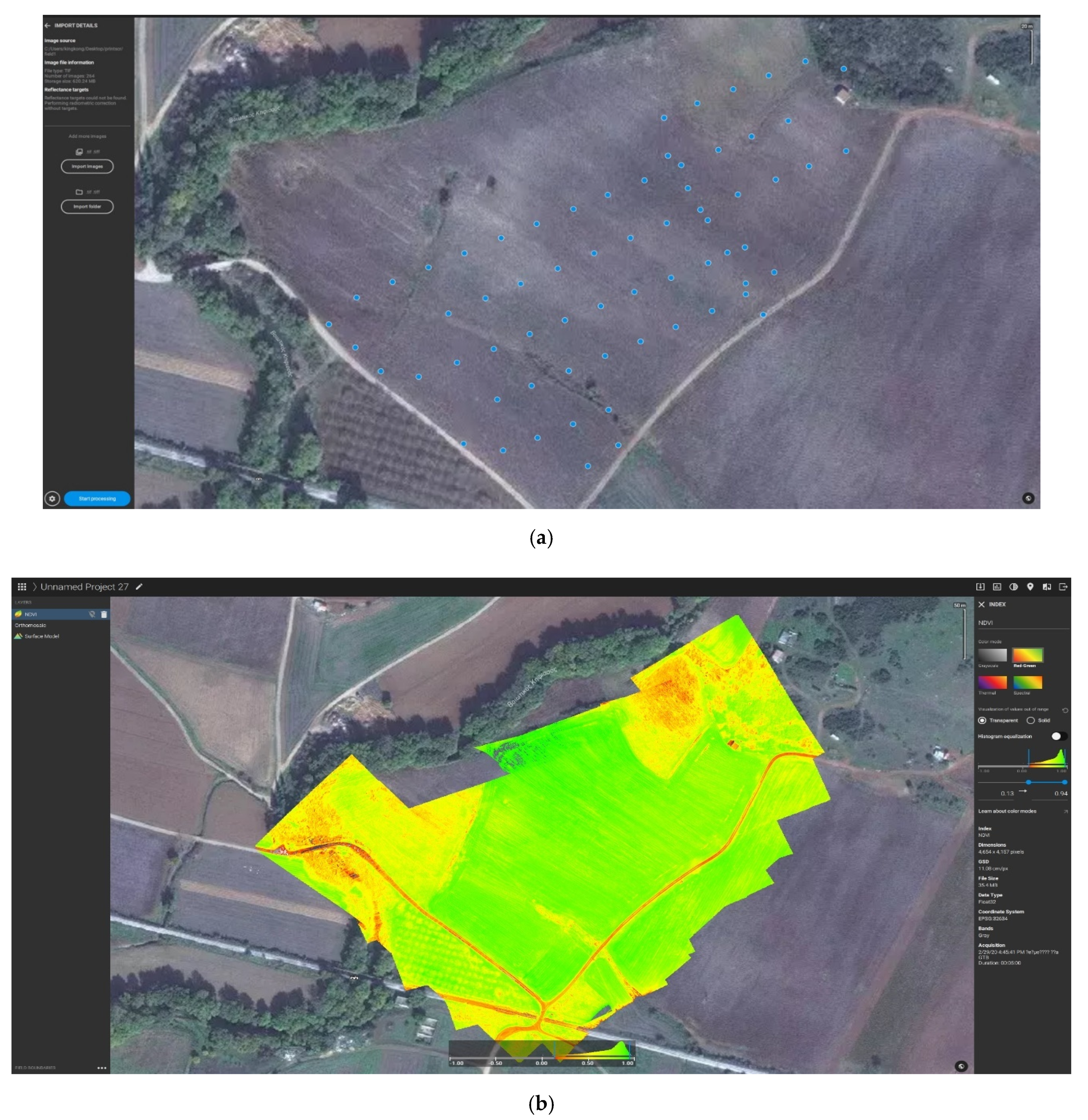
2.2. Material and Methods
3. Results and Discussion
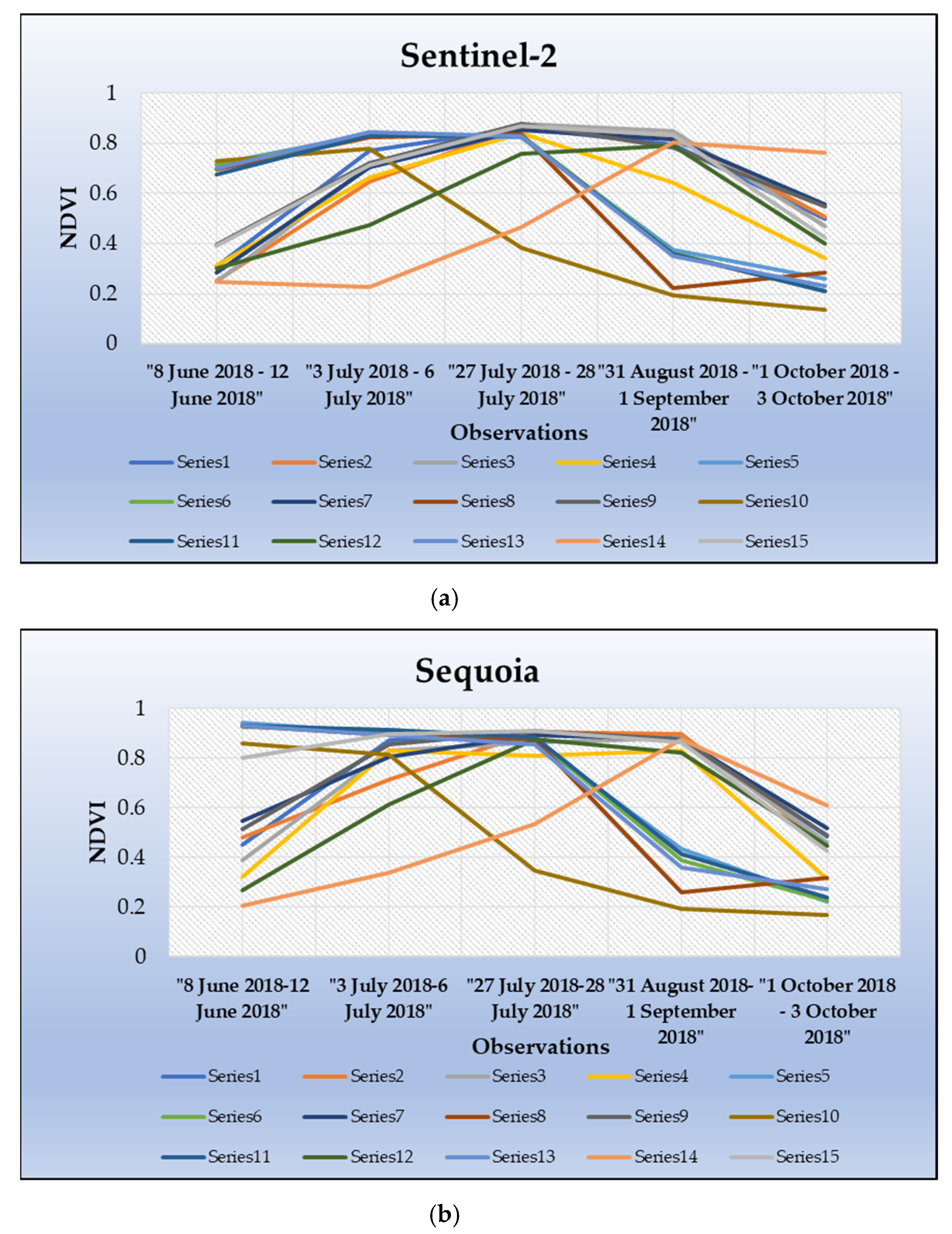
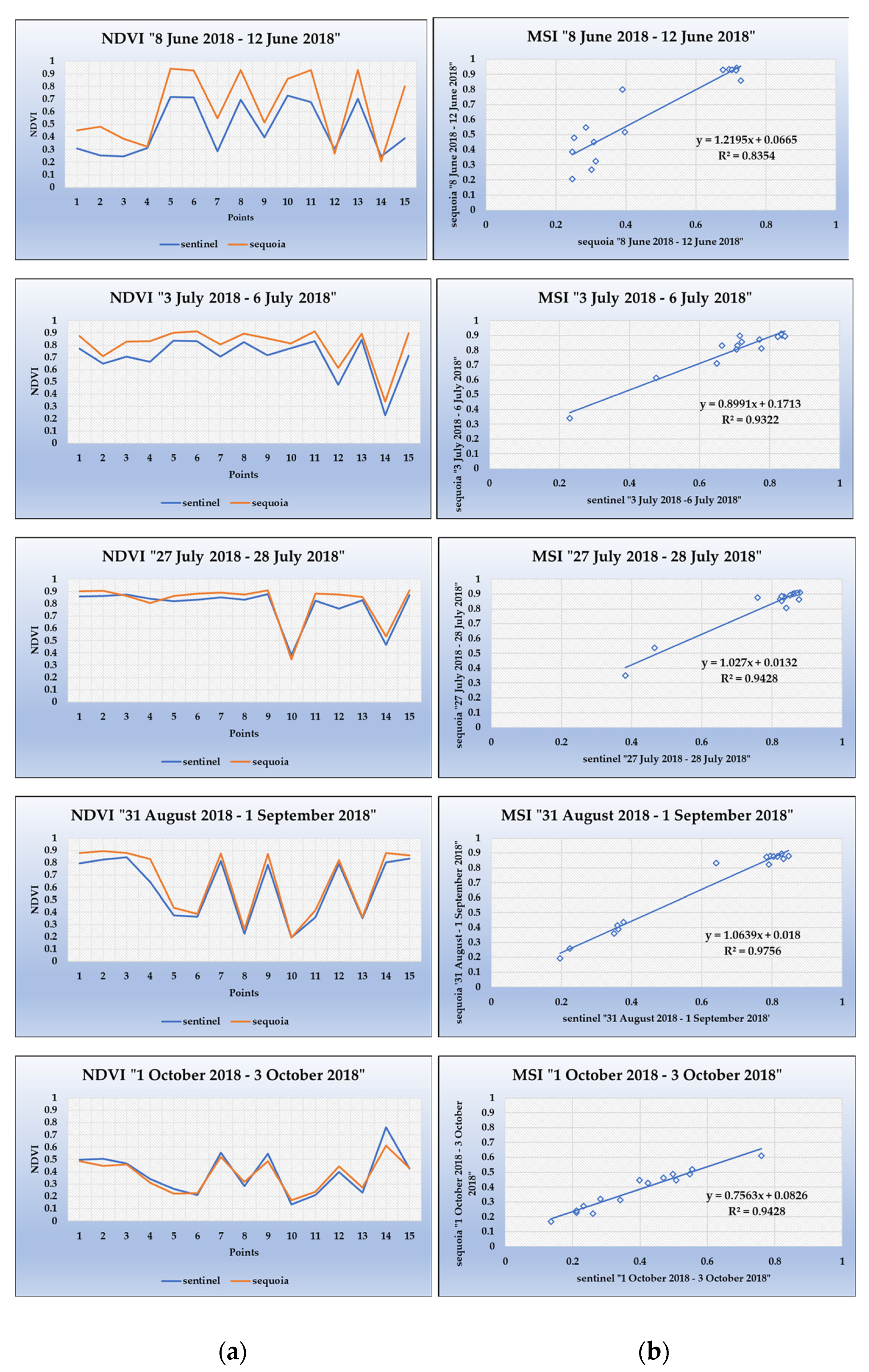
3.1. Distribution of the NDVI Values of Single Points
3.2. Distribution of the NDVI for the Selected Polygons (A, B, C, D)
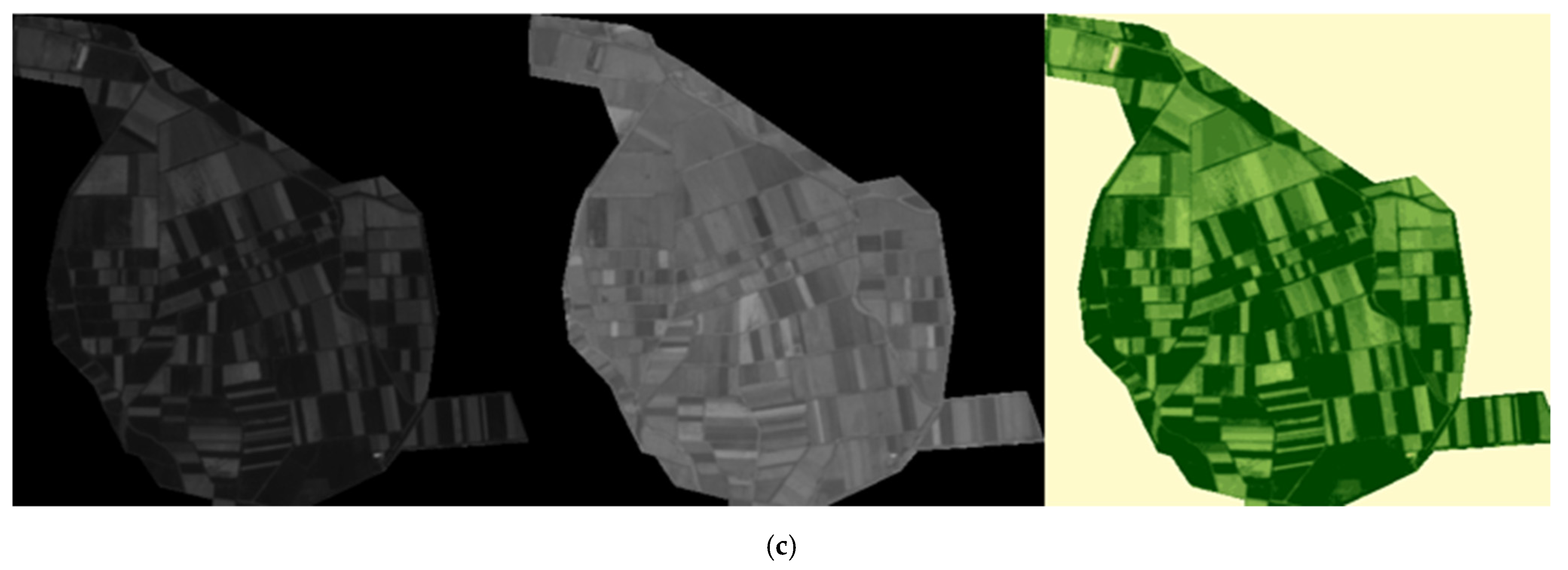
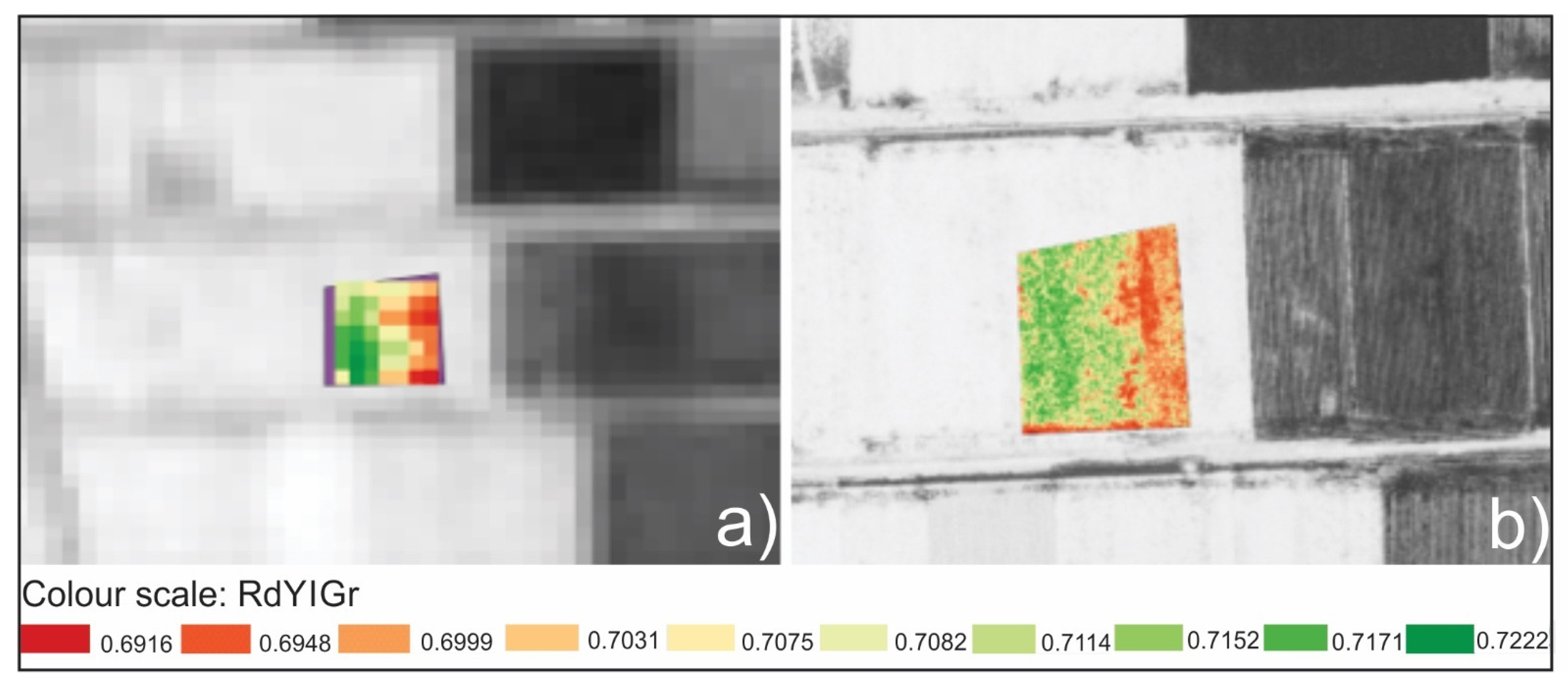
3.3. 2D Visualization of the Sentinel-2 and UAV Multispectral Data
3.4. The Use of Sentinel-2 and UAV Multispectral Data in Precision Agriculture
- The use of Sentinel-2 platform is proved effective to describe the vegetation and the vigority of the plants presenting a quite similar behavior to the UAVs’ data regarding the NDVI trend.
- Sentinel-2 imagery does not always manage to detect localized conditions, especially in areas showing high heterogeneity due to abiotic or biotic stress. In such cases, the use of UAV is necessary.
4. Conclusions
- The trend of the average NDVI is almost identical for both remote sensing techniques.
- There is a strong correlation of the NDVI index between the two techniques.
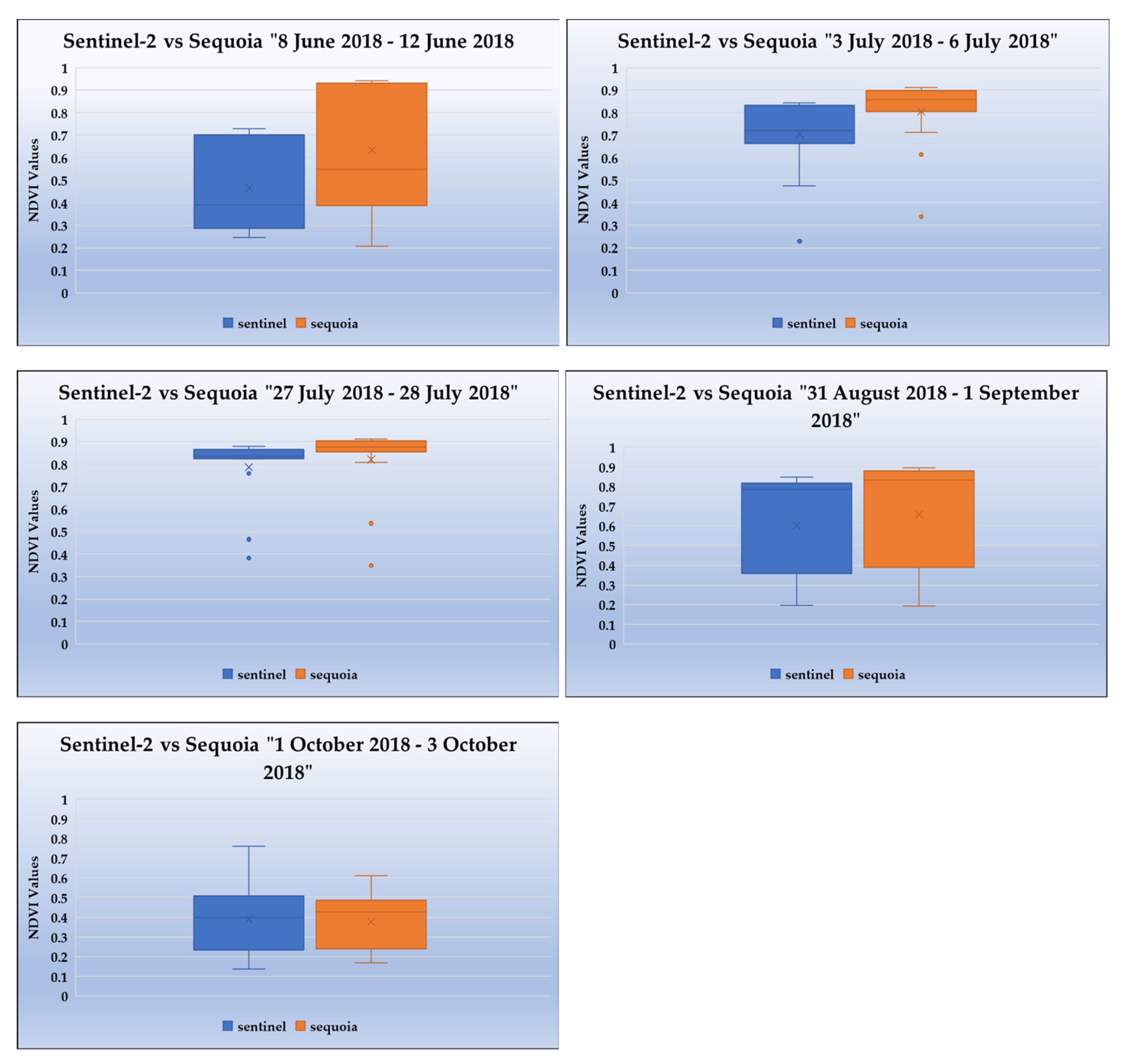
- Four out of five observations indicated statistical significance for the mean values of the NDVI index for the fifteen points, with the UAV multispectral data to present the higher ones. Considering the polygons, one polygon from the four showed statistical significance of the NDVI mean between the techniques.
- The range of the NDVI values (max, min) is larger and the coefficient of variability (CV) is higher for the UAV multispectral data compared to Sentinel-2 data due to the higher spatial resolution of the UAV’s sensor.
- The multispectral camera of the UAV is recommended for localized operations because it is more analytic and effective compared to the satellite’s sensor.
Author Contributions
Funding
Institutional Review Board Statement
Informed Consent Statement
Data Availability Statement
Acknowledgments
Conflicts of Interest
Appendix A
| Points | Latitude | Longitude |
|---|---|---|
| 1 | 41.16315733422939 | 23.284849229390677 |
| 2 | 41.16000865143369 | 23.291834238351253 |
| 3 | 41.15581040770609 | 23.28879413082437 |
| 4 | 41.156606626344086 | 23.298964014336914 |
| 5 | 41.148354905913976 | 23.287961720430104 |
| 6 | 41.15262553315412 | 23.295489605734765 |
| 7 | 41.153132217741934 | 23.305912831541217 |
| 8 | 41.14770345430107 | 23.294440044802865 |
| 9 | 41.14991115143369 | 23.30312606630824 |
| 10 | 41.14285375896058 | 23.295200071684587 |
| 11 | 41.14488049731183 | 23.302402231182793 |
| 12 | 41.14839109767025 | 23.309785349462363 |
| 13 | 41.138981241039424 | 23.29918116487455 |
| 14 | 41.142564224910394 | 23.30837387096774 |
| 15 | 41.141695622759855 | 23.317168467741933 |
| Coordinates | ||||
|---|---|---|---|---|
| Polygon | North | South | East | West |
| A | 41.158072392 | 41.157619996 | 23.293670970 | 23.293200477 |
| B | 41.148617296 | 41.148029180 | 23.282459357 | 23.287826001 |
| C | 41.145260511 | 41.144618107 | 23.298412090 | 23.297670159 |
| D | 41.145423374 | 41.144563819 | 23.304519449 | 23.303677991 |
| Descriptive Statisticssentinel_1; Sequoia_1; Sentinel_2; … _5; Sequoia_5 | ||||||
|---|---|---|---|---|---|---|
| Variable | Mean | SE Mean | Standard Deviation | Minimum | Median | Maximum |
| sentinel_1 | 0.465 | 0.0537 | 0.2079 | 0.2465 | 0.3902 | 0.7286 |
| sequoia_1 | 0.6336 | 0.0716 | 0.2773 | 0.2064 | 0.5482 | 0.9417 |
| sentinel_2 | 0.7052 | 0.0424 | 0.1642 | 0.2287 | 0.7195 | 0.8429 |
| sequoia_2 | 0.8053 | 0.0395 | 0.1529 | 0.3389 | 0.8571 | 0.9114 |
| sentinel_3 | 0.7863 | 0.039 | 0.151 | 0.3817 | 0.8342 | 0.8789 |
| sequoia_3 | 0.8207 | 0.0412 | 0.1597 | 0.3489 | 0.8768 | 0.9107 |
| sentinel_4 | 0.6004 | 0.0653 | 0.2531 | 0.1958 | 0.7841 | 0.8472 |
| sequoia_4 | 0.6567 | 0.0704 | 0.2726 | 0.1939 | 0.8315 | 0.8951 |
| sentinel_5 | 0.3888 | 0.044 | 0.1704 | 0.1362 | 0.3984 | 0.7601 |
| sequoia_5 | 0.3766 | 0.0343 | 0.1327 | 0.1677 | 0.4279 | 0.6115 |
| Observation | Descriptive Statistics | Estimation for Paired Difference | Test | ||||||||
|---|---|---|---|---|---|---|---|---|---|---|---|
| µ_Difference: Mean of (Sentinel-2–Sequoia) | Null Hypothesis H₀: μ_Difference = 0 Alternative Hypothesis H₁: μ_Difference ≠ 0 | ||||||||||
| Sample | N | Mean | StDev | SE Mean | Mean | StDev | SE Mean | 95% CI for μ_Difference | T-Value | p-Value | |
| 8 June 2018–12 June 2018 | sentinel-2 | 15 | 0.465 | 0.2079 | 0.0537 | −0.1686 | 0.1214 | 0.0314 | (−0.2358; −0.1013) | −5.38 | 0.000 |
| sequoia | 15 | 0.6336 | 0.2773 | 0.0716 | |||||||
| 3 July 2018– 6 July 2018 | sentinel-2 | 15 | 0.7052 | 0.1642 | 0.0424 | −0.1001 | 0.0431 | 0.0111 | (−0.1240; −0.0763) | −9 | 0.000 |
| sequoia | 15 | 0.8053 | 0.1529 | 0.0395 | |||||||
| 27 July 2018–28 July 2018 | sentinel-2 | 15 | 0.7863 | 0.151 | 0.039 | −0.0344 | 0.03843 | 0.00992 | (−0.05567; −0.01311) | −3.47 | 0.004 |
| sequoia | 15 | 0.8207 | 0.1597 | 0.0412 | |||||||
| 31 August 2018–1 September 2018 | sentinel-2 | 15 | 0.6004 | 0.2531 | 0.0653 | −0.0563 | 0.0455 | 0.0118 | (−0.0816; −0.0311) | −4.79 | 0.000 |
| sequoia | 15 | 0.6567 | 0.2726 | 0.0704 | |||||||
| 1 October 2018–3 October 2018 | sentinel-2 | 15 | 0.3888 | 0.1704 | 0.044 | 0.0122 | 0.0523 | 0.0135 | (−0.0168; 0.0411) | 0.9 | 0.382 |
| sequoia | 15 | 0.3766 | 0.1327 | 0.0343 | |||||||
| Area | Platform | Sensing Date | MAX | MEAN | MIN | STDDEV | CV |
|---|---|---|---|---|---|---|---|
| A | Sentinel-2 | 8 June 2018–12 June 2018 | 0.424764931 | 0.409668865 | 0.398896009 | 0.00590227 | 1.44% |
| Sentinel-2 | 3 July 2018–6 July 2018 | 0.842377245 | 0.838002589 | 0.83181119 | 0.002107325 | 0.25% | |
| Sentinel-2 | 27 July 2018–28 July 2018 | 0.862135291 | 0.851049562 | 0.828952312 | 0.009149611 | 1.08% | |
| Sentinel-2 | 31 August 2018–1 September 2018 | 0.703845322 | 0.690205042 | 0.657489479 | 0.009797661 | 1.42% | |
| Sentinel-2 | 1 October 2018–3 October 2018 | 0.466080695 | 0.451860976 | 0.419669837 | 0.011385355 | 2.52% | |
| Sequoia | 8 June 2018–12 June 2018 | 0.739971459 | 0.386712345 | 0.267078608 | 0.039826689 | 10.30% | |
| Sequoia | 3 July 2018–6 July 2018 | 0.918028831 | 0.896014414 | 0.840995193 | 0.008689196 | 0.97% | |
| Sequoia | 27 July 2018–28 July 2018 | 0.920731068 | 0.888997866 | 0.685243845 | 0.019670044 | 2.21% | |
| Sequoia | 31 August 2018–1 September 2018 | 0.856916368 | 0.712623024 | 0.432811826 | 0.062304516 | 8.74% | |
| Sequoia | 1 October 2018–3 October 2018 | 0.776085019 | 0.579790769 | 0.353510261 | 0.065478958 | 11.29% | |
| B | Sentinel-2 | 8 June 2018–12 June 2018 | 0.72285974 | 0.707651934 | 0.6915797 | 0.008361191 | 1.18% |
| Sentinel-2 | 3 July 2018–6 July 2018 | 0.840008736 | 0.833387507 | 0.822145224 | 0.00401236 | 0.48% | |
| Sentinel-2 | 27 July 2018–28 July 2018 | 0.843239069 | 0.827542223 | 0.805931032 | 0.007401045 | 0.89% | |
| Sentinel-2 | 31 August 2018–1 September 2018 | 0.426836431 | 0.38117364 | 0.349979818 | 0.017986821 | 4.72% | |
| Sentinel-2 | 1 October 2018–3 October 2018 | 0.292903215 | 0.24251502 | 0.214875594 | 0.018805529 | 7.75% | |
| Sequoia | 8 June 2018–12 June 2018 | 0.957545161 | 0.929184155 | 0.725212157 | 0.01313116 | 1.41% | |
| Sequoia | 3 July 2018–6 July 2018 | 0.931631625 | 0.898681251 | 0.770359695 | 0.011027217 | 1.23% | |
| Sequoia | 27 July 2018–28 July 2018 | 0.927700162 | 0.882190463 | 0.694832087 | 0.017135325 | 1.94% | |
| Sequoia | 31 August 2018–1 September 2018 | 0.731545687 | 0.445202932 | 0.280894756 | 0.045929647 | 10.32% | |
| Sequoia | 1 October 2018–3 October 2018 | 0.607119501 | 0.262282414 | 0.174537793 | 0.043217779 | 16.48% | |
| C | Sentinel-2 | 8 June 2018–12 June 2018 | 0.206350893 | 0.184016948 | 0.163822144 | 0.009934681 | 5.40% |
| Sentinel-2 | 3 July 2018–6 July 2018 | 0.579889655 | 0.377094243 | 0.176204428 | 0.095115443 | 25.22% | |
| Sentinel-2 | 27 July 2018–28 July 2018 | 0.772020161 | 0.585997589 | 0.290901035 | 0.096564769 | 16.48% | |
| Sentinel-2 | 31 August 2018–1 September 2018 | 0.492080986 | 0.41989237 | 0.315348059 | 0.049551697 | 11.80% | |
| Sentinel-2 | 1 October 2018–3 October 2018 | 0.591126442 | 0.379471433 | 0.214191154 | 0.121058057 | 31.90% | |
| Sequoia | 8 June 2018–12 June 2018 | 0.802700639 | 0.185702369 | 0.121396981 | 0.056253917 | 30.29% | |
| Sequoia | 3 July 2018–6 July 2018 | 0.89239186 | 0.455740255 | 0.101822048 | 0.236436583 | 51.88% | |
| Sequoia | 27 July 2018–28 July 2018 | 0.902240813 | 0.694348733 | 0.130899876 | 0.191690991 | 27.61% | |
| Sequoia | 31 August 2018–1 September 2018 | 0.868877113 | 0.539666935 | 0.16559723 | 0.140022944 | 25.95% | |
| Sequoia | 1 October 2018–3 October 2018 | 0.85949403 | 0.472400034 | 0.164854422 | 0.180505956 | 38.21% | |
| D | Sentinel-2 | 8 June 2018–12 June 2018 | 0.290092528 | 0.270967551 | 0.248297825 | 0.010585632 | 3.91% |
| Sentinel-2 | 3 July 2018–6 July 2018 | 0.602515101 | 0.515073871 | 0.366025954 | 0.065445929 | 12.71% | |
| Sentinel-2 | 27 July 2018–28 July 2018 | 0.869380832 | 0.835450653 | 0.770878434 | 0.026236285 | 3.14% | |
| Sentinel-2 | 31 August 2018–1 September 2018 | 0.856839776 | 0.840226661 | 0.822994411 | 0.006889503 | 0.82% | |
| Sentinel-2 | 1 October 2018–3 October 2018 | 0.72909236 | 0.596489981 | 0.524814963 | 0.055854803 | 9.36% | |
| Sequoia | 8 June 2018–12 June 2018 | 0.73825258 | 0.342425083 | 0.18140173 | 0.099854429 | 29.16% | |
| Sequoia | 3 July 2018–6 July 2018 | 0.903458595 | 0.691964177 | 0.192108214 | 0.150160703 | 21.70% | |
| Sequoia | 27 July 2018–28 July 2018 | 0.9346416 | 0.890634058 | 0.378713846 | 0.042593657 | 4.78% | |
| Sequoia | 31 August 2018–1 September 2018 | 0.927322805 | 0.883830221 | 0.603708208 | 0.013481126 | 1.53% | |
| Sequoia | 1 October 2018–3 October 2018 | 0.81042999 | 0.602571672 | 0.282279491 | 0.084460655 | 14.02% |
| ANOVA: NDVI_MEAN versus Sensing Platforms; Observations | |||||||||||||
|---|---|---|---|---|---|---|---|---|---|---|---|---|---|
| Areas | Factor Information | Analysis of Variance for NDVI_MEAN_Areas | Model Summary | ||||||||||
| Factor | Type | Levels | Values | Source | DF | SS | MS | F | P | S | R-sq | R-sq(adj) | |
| A | Sensing Platforms | Fixed | 2 | Sentinel-2; Sequoia | Sensing Platform | 1 | 0.00499 | 0.00499 | 3.26 | 0.145 | 0.0390 | 0.983 | 0.962 |
| Observations | Fixed | 5 | 1,2,3,4,5 | Observations | 4 | 0.35492 | 0.08873 | 58.07 | 0.001 | ||||
| Error | 4 | 0.00611 | 0.00153 | ||||||||||
| Total | 9 | 0.36602 | |||||||||||
| B | Sensing Platforms | Fixed | 2 | Sentinel-2; Sequoia | Sensing Platform | 1 | 0.01809 | 0.01809 | 5.87 | 0.073 | 0.0555 | 0.982 | 0.959 |
| Observations | Fixed | 5 | 1,2,3,4,5 | Observations | 4 | 0.66153 | 0.16538 | 53.68 | 0.001 | ||||
| Error | 4 | 0.01232 | 0.00308 | ||||||||||
| Total | 9 | 0.69194 | |||||||||||
| C | Sensing Platforms | Fixed | 2 | Sentinel-2; Sequoia | Sensing Platform | 1 | 0.01611 | 0.01611 | 14.84 | 0.018 | 0.0329 | 0.981 | 0.958 |
| Observations | Fixed | 5 | 1,2,3,4,5 | Observations | 4 | 0.21389 | 0.05347 | 49.24 | 0.001 | ||||
| Error | 4 | 0.00434 | 0.00109 | ||||||||||
| Total | 9 | 0.23434 | |||||||||||
| D | Sensing Platforms | Fixed | 2 | Sentinel-2; Sequoia | Sensing Platform | 1 | 0.01248 | 001248 | 6.08 | 0.069 | 0.0453 | 0.981 | 0.958 |
| Observations | Fixed | 5 | 1,2,3,4,5 | Observations | 4 | 0.42572 | 0.10643 | 51.83 | 0.001 | ||||
| Error | 4 | 0.00821 | 0.00205 | ||||||||||
| Total | 9 | 0.44641 | |||||||||||
References
- Pinter, P.J.; Hatfield, J.L.; Schepers, J.S.; Barnes, E.M.; Moran, M.S.; Daughtry, C.S.T.; Upchurch, D.R. Remote Sensing for Crop Management. Photogramm. Eng. Remote Sens. 2003, 69, 647–664. [Google Scholar] [CrossRef]
- Gomarasca, M.A. Basics of Geomatics, 1st ed.; Springer: Dordrecht, The Netherlands, 2009. [Google Scholar] [CrossRef]
- Ravelo, A.C.; Abril, E.G. Remote Sensing. In Applied Agrometeorology; Stigter, K., Ed.; Springer: Berlin/Heidelberg, Germany, 2010; pp. 1013–1024. [Google Scholar] [CrossRef]
- Jones, H.G.; Vaughan, R.A. Remote Sensing of Vegetation Principles, Techniques, and Applications; Oxford University Press: Oxford, UK, 2010; ISBN 9780199207794. [Google Scholar]
- Kingra, P.K.; Majumder, D.; Singh, S.P. Application of Remote Sensing and GIS in Agriculture and Natural Resource Management Under Changing Climatic Conditions. Agric. Res. J. 2016, 53, 295–302. [Google Scholar] [CrossRef]
- Mani, J.K.; Varghese, A.O. Remote Sensing and GIS in Agriculture and Forest Resource Monitoring. In Geospatial Technologies in Land Resources Mapping, Monitoring and Management, Geotechnologies and the Environment, 1st ed.; Reddy, G., Singh, S., Eds.; Springer International Publishing: Cham, Switzerland, 2018; Volume 21, pp. 377–400. [Google Scholar] [CrossRef]
- Shanmugapriya, P.; Rathika, S.; Ramesh, T.; Janaki, P. Applications of Remote Sensing in Agriculture—A Review. Int. J. Curr. Microbiol. App. Sci. 2019, 8, 2270–2283. [Google Scholar] [CrossRef]
- Strickland, R.M.; Ess, D.R.; Parsons, S.D. Precision Farming and Precision Pest Management: The Power of New Crop Production Technologies. J. Nematol. 1998, 30, 431–435. [Google Scholar]
- Singh, A.K. Precision Farming; I.A.R.I.: New Delhi, India, 2001. [Google Scholar]
- Robert, P.C. Precision agriculture: A challenge for crop nutrition management. Plant Soil 2002, 247, 143–149. [Google Scholar] [CrossRef]
- Zhang, M.; Li, M.Z.; Liu, G.; Wang, M.H. Yield Mapping in Precision Farming. In Computer and Computing Technologies in Agriculture, Volume II. CCTA 2007. The International Federation for Information Processing; Li, D., Ed.; Springer: Boston, MA, USA, 2007; Volume 259, pp. 1407–1410. [Google Scholar] [CrossRef]
- Goswami, S.B.; Matin, S.; Saxena, A.; Bairagi, G.D. A Review: The application of Remote Sensing, GIS and GPS in Precision Agriculture. Int. J. Adv. Technol. Eng. Res. 2012, 2, 50–54. [Google Scholar]
- Heege, H.J.; Thiessen, E. Sensing of Crop Properties. In Precision in Crop Farming: Site Specific Concepts and Sensing Methods: Applications and Results; Heege, H., Ed.; Springer Science + Business Media: Dordrecht, The Nenderlands, 2013; pp. 103–141. [Google Scholar] [CrossRef]
- Zude-Sasse, M.; Fountas, S.; Gemtos, T.A.; Abu-Khalaf, N. Applications of precision agriculture in horticultural crops. Eur. J. Hortic. Sci. 2016, 81, 78–90. [Google Scholar] [CrossRef]
- Balafoutis, A.; Beck, B.; Fountas, S.; Vangeyte, J.; van der Wal, T.; Soto, I.; Gomez-Barbero, M.; Barnes, A.; Eory, V. Precision Agriculture Technologies Positively Contributing to GHG Emissions Mitigation, Farm Productivity and Economics. Sustainability 2017, 9, 1339. [Google Scholar] [CrossRef]
- Paustian, M.; Theuvsen, L. Adoption of precision agriculture technologies by German crop farmers. Precis. Agric. 2017, 18, 701–716. [Google Scholar] [CrossRef]
- Pallottino, F.; Biocca, M.; Nardi, P.; Figorilli, S.; Menesatti, P.; Costa, C. Science mapping approach to analyse the research evolution on precision agriculture: World, EU and Italian situation. Precis. Agric. 2018, 19, 1011–1026. [Google Scholar] [CrossRef]
- Fulton, J.; Hawkins, E.; Taylor, R.; Franzen, A. Yield Monitoring and Mapping. In Precision Agriculture Basics; Shannon, D.K., Clay, D.E., Kitchen, N.R., Eds.; ASA, CSSA, SSSA: Madison, WI, USA, 2018; pp. 63–77. [Google Scholar] [CrossRef]
- Shafi, U.; Mumtaz, R.; García-Nieto, J.; Hassan, S.A.; Zaidi, S.A.R.; Iqbal, N. Precision Agriculture Techniques and Practices: From Considerations to Applications. Sensors 2019, 19, 3796. [Google Scholar] [CrossRef] [PubMed]
- Nandibewoor, A.; Hebbal, S.B.; Hegadi, R. Remote Monitoring of Maize Crop through Satellite Multispectral Imagery. Procedia Comput. Sci. 2015, 45, 344–353. [Google Scholar] [CrossRef]
- Escola, A.; Badia, N.; Arno, J.; Martinez-Casanovas, J.A. Using Sentinel-2 images to implement Precision Agriculture techniques in large arable fields: First results of a case study. Adv. Anim. Biosci. 2017, 8, 377–382. [Google Scholar] [CrossRef]
- Belgiu, M.; Csillik, O. Sentinel-2 cropland mapping using pixel-based and object-based time-weighted dynamic time warping analysis. Remote Sens. Environ. 2018, 204, 509–523. [Google Scholar] [CrossRef]
- Ahmad, L.; Mahdi, S.S. Satellite Farming; Springer International Publishing: Cham, Switzerland, 2018; ISBN 978-3-030-03448-1. [Google Scholar] [CrossRef]
- Rapinel, S.; Mony, C.; Lecoq, L.; Clément, B.; Thomas, A.; Hubert-Moy, L. Evaluation of Sentinel-2 time-series for mapping floodplain grassland plant communities. Remote Sens. Environ. 2019, 223, 115–129. [Google Scholar] [CrossRef]
- Zhang, C.; Kovacs, J.M. The application of small unmanned aerial systems for precision agriculture: A review. Precis. Agric. 2012, 13, 693–712. [Google Scholar] [CrossRef]
- Anderson, K.; Gaston, K.J. Lightweight unmanned aerial vehicles will revolutionize spatial ecology. Front. Ecol. Environ. 2013, 11, 138–146. [Google Scholar] [CrossRef]
- Csillik, O.; Cherbini, J.; Johnson, R.; Lyons, A.; Kelly, M. Identification of Citrus Trees from Unmanned Aerial Vehicle Imagery Using Convolutional Neural Networks. Drones 2018, 2, 39. [Google Scholar] [CrossRef]
- Barbedo, J.G. A Review on the Use of Unmanned Aerial Vehicles and Imaging Sensors for Monitoring and Assessing Plant Stresses. Drones 2019, 3, 40. [Google Scholar] [CrossRef]
- Mesas-Carrascosa, F.J.; Notario-Garcia, M.D.; de Larriva, J.E.M.; de la Orden, M.S.; Garcia-Ferrer Porras, A. Validation of measurements of land plot area using UAV imagery. Int. J. Appl. Earth Obs. Geoinf. 2014, 33, 270–279. [Google Scholar] [CrossRef]
- Rokhmana, C.A. The potential of UAV-based remote sensing for supporting precision agriculture in Indonesia. Procedia Environ. Sci. 2015, 24, 245–253. [Google Scholar] [CrossRef]
- Yun, G.; Mazur, M.; Pederii, Y. Role of Unmanned Aerial Vehicles in Precision Farming. Proc. Natl. Aviat. Univ. 2017, 10, 106–112. [Google Scholar] [CrossRef]
- Manfreda, S.; McCabe, M.E.; Miller, P.E.; Lucas, R.; Madrigal, V.P.; Mallinis, G.; Dor, E.B.; Helman, D.; Estes, L.; Ciraolo, G.; et al. On the Use of Unmanned Aerial Systems for Environmental Monitoring. Remote Sens. 2018, 10, 641. [Google Scholar] [CrossRef]
- Maes, W.H.; Steppe, K. Perspectives for Remote Sensing with Unmanned Aerial Vehicles in Precision Agriculture. Trends Plant. Sci. 2019, 24, 152–164. [Google Scholar] [CrossRef]
- Radoglou-Grammatikis, P.; Sarigiannidis, P.; Lagkas, T.; Moscholios, I. A compilation of UAV applications for precision agriculture. Comput. Netw. 2020, 172, 107148. [Google Scholar] [CrossRef]
- Ozdarici-Ok, A. Automatic detection and delineation of citrus trees from VHR satellite imagery. Int. J. Remote Sens. 2015, 36, 4275–4296. [Google Scholar] [CrossRef]
- Pérez-Ortiz, M.; Peña, J.M.; Gutiérrez, P.A.; Torres-Sánchez, J.; Hervás-Martínez, C.; López-Granados, F. A semi-supervised system for weed mapping in sunflower crops using unmanned aerial vehicles and a crop row detection method. Appl. Soft. Comput. 2015, 37, 533–544. [Google Scholar] [CrossRef]
- Torres-Sánchez, J.; López-Granados, F.; Peña, J.M. An automatic object-based method for optimal thresholding in UAV images Application for vegetation detection in herbaceous crops. Comput. Electron. Agric. 2015, 114, 43–52. [Google Scholar] [CrossRef]
- Panagiotakis, C.; Kokinou, E. Unsupervised Detection of Topographic Highs with Arbitrary Basal Shapes Based on Volume Evolution of Isocontours. Comput. Geosci. 2017, 102, 22–33. [Google Scholar] [CrossRef]
- De Castro, A.I.; Torres-Sánchez, J.; Peña, J.M.; Jiménez-Brenes, F.M.; Csillik, O.; López-Granados, F. An automatic random forest-OBIA algorithm for early weed mapping between and within crop rows using UAV imagery. Remote Sens. 2018, 10, 285. [Google Scholar] [CrossRef]
- Georgi, C.; Spengler, D.; Itzerott, S.; Kleinschmit, B. Automatic delineation algorithm for site-specific management zones based on satellite remote sensing data. Precis. Agric. 2018, 19, 684–707. [Google Scholar] [CrossRef]
- Louargant, M.; Jones, G.; Faroux, R.; Paoli, J.-N.; Maillot, T.; Gée, C.; Villette, S. Unsupervised classification algorithm for early weed detection in row-crops by combining spatial and spectral information. Remote Sens. 2018, 10, 761. [Google Scholar] [CrossRef]
- Haboudane, D.; Miller, J.R.; Tremblay, N.; Zarco-Tejada, P.J.; Dextraze, L. Integrated narrowband vegetation indices for prediction of crop chlorophyll content for application to precision agriculture. Remote Sens. Environ. 2002, 81, 416–426. [Google Scholar] [CrossRef]
- Tarnavsky, E.; Garrigues, S.; Brown, M.E. Multiscale geostatistical analysis of AVHRR, SPOT-VGT, and MODIS global NDVI products. Remote Sens. Environ. 2008, 112, 535–549. [Google Scholar] [CrossRef]
- Anderson, J.H.; Weber, K.T.; Gokhale, B.; Chen, F. Intercalibration and Evaluation of ResourceSat-1 and Landsat-5 NDVI. Can. J. Remote Sens. 2011, 37, 213–219. [Google Scholar] [CrossRef]
- Simms, É.L.; Ward, H. Multisensor NDVI-Based Monitoring of the Tundra-Taiga Interface (Mealy Mountains, Labrador, Canada). Remote Sens. 2013, 5, 1066–1090. [Google Scholar] [CrossRef]
- Houborg, R.; McCabe, M.F. High-Resolution NDVI from planet’s constellation of earth observing nano-satellites: A new data source for precision agriculture. Remote Sens. 2016, 8, 768. [Google Scholar] [CrossRef]
- Fawcett, D.; Panigada, C.; Tagliabue, G.; Boschetti, M.; Celesti, M.; Evdokimov, A.; Biriukova, K.; Colombo, R.; Miglietta, F.; Rascher, U.; et al. Multi-Scale Evaluation of Drone-Based Multispectral Surface Reflectance and Vegetation Indices in Operational Conditions. Remote Sens. 2020, 12, 514. [Google Scholar] [CrossRef]
- European Space Agency. Sentinel-2 User Handbook; European Space Agency: Paris, France, 2015; pp. 53–54. [Google Scholar]
- Fletcher, K. Sentinel-2. ESA’s Optical High-Resolution Mission for GMES Operational Services; ESA Communications: Noordwijk, The Netherlands, 2012; ISBN 978-92-9221-419-7. [Google Scholar]
- Ünsalan, C.; Boyer, K.L. (Eds.) Remote Sensing Satellites and Airborne Sensors. In Multispectral Satellite Image Understanding. Advances in Computer Vision and Pattern Recognition; Springer: London, UK, 2011; pp. 7–15. [Google Scholar] [CrossRef]
- Matese, A.; Toscano, P.; Di Gennaro, S.F.; Genesio, L.; Vaccari, F.P.; Primicerio, J.; Belli, C.; Zaldei, A.; Bianconi, R.; Gioli, B. Intercomparison of UAV, aircraft and satellite remote sensing platforms for precision viticulture. Remote Sens. 2015, 7, 2971–2990. [Google Scholar] [CrossRef]
- McCabe, M.F.; Houborg, R.; Lucieer, A. High-resolution sensing for precision agriculture: From Earth-observing satellites to unmanned aerial vehicles. Remote Sens. Agric. Ecosyst. Hydrol. XVIII 2016, 9998, 999811. [Google Scholar]
- Benincasa, P.; Antognelli, S.; Brunetti, L.; Fabbri, C.A.; Natale, A.; Sartoretti, V.; Modeo, G.; Guiducci, M.; Tei, F.; Vizzari, M. Reliability of Ndvi Derived by High Resolution Satellite and Uav Compared To in-Field Methods for the Evaluation of Early Crop N Status and Grain Yield in Wheat. Exp. Agric. 2017, 54, 1–19. [Google Scholar] [CrossRef]
- Borgogno-Mondino, E.; Lessio, A.; Tarricone, L.; Novello, V.; de Palma, L. A comparison between multispectral aerial and satellite imagery in precision viticulture. Precis. Agric. 2018, 19, 195. [Google Scholar] [CrossRef]
- Malacarne, D.; Pappalardo, S.E.; Codato, D. Sentinel-2 Data Analysis and Comparison with UAV Multispectral Images for Precision Viticulture. GI Forum 2018, 105–116. [Google Scholar]
- Khaliq, A.; Comba, L.; Biglia, A.; Ricauda Aimonino, D.; Chiaberge, M.; Gay, P. Comparison of Satellite and UAV-Based Multispectral Imagery for Vineyard Variability Assessment. Remote Sens. 2019, 11, 436. [Google Scholar] [CrossRef]
- Pla, M.; Bota, G.; Duane, A.; Balagué, J.; Curcó, A.; Gutiérrez, R.; Brotons, L. Calibrating Sentinel-2 Imagery with Multispectral UAV Derived Information to Quantify Damages in Mediterranean Rice Crops Caused by Western Swamphen (Porphyrio porphyrio). Drones 2019, 3, 45. [Google Scholar] [CrossRef]
- Messina, G.; Peña, J.M.; Vizzari, M.; Modica, G. A Comparison of UAV and Satellites Multispectral Imagery in Monitoring Onion Crop. An Application in the ’Cipolla Rossa di Tropea’ (Italy). Remote Sens. 2020, 12, 3424. [Google Scholar] [CrossRef]


| Sensing Platform | Band Number | Band | Central Wavelength (nm) | Bandwith (nm) | Spatial Resolution |
|---|---|---|---|---|---|
| Sentinel 2 | 1 | Violet | 443 | 20 | 60 |
| 2 | Blue | 490 | 65 | 10 | |
| 3 | Green | 560 | 35 | 10 | |
| 4 | Red | 665 | 30 | 10 | |
| 5 | Red Edge | 705 | 15 | 20 | |
| 6 | Near Infrared | 740 | 15 | 20 | |
| 7 | 783 | 20 | 20 | ||
| 8 | 842 | 115 | 10 | ||
| 8b | 865 | 20 | 20 | ||
| 9 | 945 | 20 | 60 | ||
| 10 | 1380 | 30 | 60 | ||
| 11 | Short Wavelength Infrared | 1610 | 90 | 20 | |
| 12 | 2190 | 180 | 20 | ||
| Band | Wavelengths (nm) | ||||
| Sequoia | Green | 500–600 | |||
| Red | 600–700 | ||||
| Red Edge | 700–730 | ||||
| Near Infrared | 700–1300 | ||||
| Sensing Date | 8 June 2018– 12 June 2018 | 3 July 2018– 6 July 2018 | 27 July 2018– 28 July 2018 | 31 August 2018– 1 September 2018 | 1 October 2018– 3 October 2018 | |||||
|---|---|---|---|---|---|---|---|---|---|---|
| Points | Sentinel-2 | Sequoia | Sentinel-2 | Sequoia | Sentinel-2 | Sequoia | Sentinel-2 | Sequoia | Sentinel-2 | Sequoia |
| 1 | 0,30878 | 0,45173 | 0,77035 | 0,8728 | 0,85896 | 0,90208 | 0,79467 | 0,87877 | 0,49705 | 0,48634 |
| 2 | 0,25231 | 0,48002 | 0,64824 | 0,71208 | 0,86481 | 0,90465 | 0,82728 | 0,89512 | 0,50721 | 0,447 |
| 3 | 0,24722 | 0,38731 | 0,70826 | 0,82971 | 0,87684 | 0,86197 | 0,84717 | 0,88098 | 0,46924 | 0,46107 |
| 4 | 0,31391 | 0,32423 | 0,66333 | 0,83165 | 0,84006 | 0,80724 | 0,64111 | 0,83148 | 0,34081 | 0,31222 |
| 5 | 0,7164 | 0,94173 | 0,83557 | 0,90238 | 0,82301 | 0,86537 | 0,37613 | 0,43533 | 0,25952 | 0,22123 |
| 6 | 0,71396 | 0,92676 | 0,83349 | 0,91139 | 0,83356 | 0,88134 | 0,36238 | 0,38788 | 0,21086 | 0,22788 |
| 7 | 0,28583 | 0,54815 | 0,70521 | 0,80471 | 0,85147 | 0,89067 | 0,81502 | 0,8751 | 0,55524 | 0,51996 |
| 8 | 0,69419 | 0,93194 | 0,8237 | 0,89235 | 0,83424 | 0,87595 | 0,22414 | 0,25971 | 0,28267 | 0,31891 |
| 9 | 0,39736 | 0,51542 | 0,71945 | 0,85713 | 0,87891 | 0,91071 | 0,78413 | 0,87402 | 0,5481 | 0,48804 |
| 10 | 0,72855 | 0,85989 | 0,77669 | 0,81172 | 0,38167 | 0,34895 | 0,19581 | 0,19394 | 0,13616 | 0,16768 |
| 11 | 0,67647 | 0,93175 | 0,83293 | 0,91139 | 0,82726 | 0,88462 | 0,35944 | 0,41533 | 0,21148 | 0,23982 |
| 12 | 0,30092 | 0,26731 | 0,47523 | 0,61353 | 0,75925 | 0,87675 | 0,79089 | 0,8238 | 0,39836 | 0,44632 |
| 13 | 0,70188 | 0,93056 | 0,84293 | 0,89344 | 0,82767 | 0,85523 | 0,35015 | 0,36003 | 0,2318 | 0,27342 |
| 14 | 0,24646 | 0,20644 | 0,22868 | 0,33886 | 0,46538 | 0,53582 | 0,80488 | 0,8779 | 0,76006 | 0,61152 |
| 15 | 0,39024 | 0,80005 | 0,71392 | 0,89684 | 0,87108 | 0,90871 | 0,83271 | 0,86174 | 0,42353 | 0,42794 |
Publisher’s Note: MDPI stays neutral with regard to jurisdictional claims in published maps and institutional affiliations. |
© 2021 by the authors. Licensee MDPI, Basel, Switzerland. This article is an open access article distributed under the terms and conditions of the Creative Commons Attribution (CC BY) license (https://creativecommons.org/licenses/by/4.0/).
Share and Cite
Bollas, N.; Kokinou, E.; Polychronos, V. Comparison of Sentinel-2 and UAV Multispectral Data for Use in Precision Agriculture: An Application from Northern Greece. Drones 2021, 5, 35. https://doi.org/10.3390/drones5020035
Bollas N, Kokinou E, Polychronos V. Comparison of Sentinel-2 and UAV Multispectral Data for Use in Precision Agriculture: An Application from Northern Greece. Drones. 2021; 5(2):35. https://doi.org/10.3390/drones5020035
Chicago/Turabian StyleBollas, Nikolaos, Eleni Kokinou, and Vassilios Polychronos. 2021. "Comparison of Sentinel-2 and UAV Multispectral Data for Use in Precision Agriculture: An Application from Northern Greece" Drones 5, no. 2: 35. https://doi.org/10.3390/drones5020035
APA StyleBollas, N., Kokinou, E., & Polychronos, V. (2021). Comparison of Sentinel-2 and UAV Multispectral Data for Use in Precision Agriculture: An Application from Northern Greece. Drones, 5(2), 35. https://doi.org/10.3390/drones5020035


