Leveraging AI to Estimate Caribou Lichen in UAV Orthomosaics from Ground Photo Datasets

Abstract

Relating ground photographs to UAV orthomosaics is a key linkage required for accurate multi-scaled lichen mapping. Conventional methods of multi-scaled lichen mapping, such as random forest models and convolutional neural networks, heavily rely on pixel DN values for classification. However, the limited spectral range of ground photos requires additional characteristics to differentiate lichen from spectrally similar objects, such as bright logs. By applying a neural network to tiles of a UAV orthomosaics, additional characteristics, such as surface texture and spatial patterns, can be used for inferences. Our methodology used a neural network (UAV LiCNN) trained on ground photo mosaics to predict lichen in UAV orthomosaic tiles. The UAV LiCNN achieved mean user and producer accuracies of 85.84% and 92.93%, respectively, in the high lichen class across eight different orthomosaics. We compared the known lichen percentages found in 77 vegetation microplots with the predicted lichen percentage calculated from the UAV LiCNN, resulting in a R² relationship of 0.6910. This research shows that AI models trained on ground photographs effectively classify lichen in UAV orthomosaics. Limiting factors include the misclassification of spectrally similar objects to lichen in the RGB bands and dark shadows cast by vegetation.

1. Introduction

Recent studies have indicated that the mapping of caribou lichen is vital for sustainable land management and caribou recovery plans [1,2,3,4,5]. Canadian caribou are threatened by a changing environment due to declining lichen availability, unregulated hunting, habitat disturbances, and herd fragmentation due to human-made infrastructure [2,3,4,5,6]. Lichen is a dominant food source for caribou in the winter, comprising 75% and 25% of their diets in the winter and summer seasons respectively [5]. Therefore, developing a refined multi-scale approach to lichen mapping is timely for understanding Canada’s caribou food availability. The basis data for mapping caribou lichen availability consists of vegetation microplot ground photographs and UAV orthomosaics.

Digital ground photographs of vegetation microplots can be used to infer localized knowledge across broader landscapes, such as large-scale vegetation patterns and plant classifications [7]. These photographs have ultra-high spatial resolution (mm) by nature, and allow scientists or artificial intelligence to classify plant species in the survey location with high accuracy [7]. This information can be used to inform classification models operating at lower resolution over the same area, such as aerial or satellite imagery.

Unmanned Aerial Vehicles (UAVs), also known as Remotely Piloted Aircraft Systems (RPAS), are capable of collecting photographs with lower spatial resolution (1–5 cm) than the field photographs over larger regions of interest [8]. The aerial photographs collected by these systems can be used to generate high-quality landscape orthomosaics, which provide a basis for ecological applications of remote sensing, such as classifying vegetation in forests and wetlands [8,9,10,11], precision agriculture [12], and multi-scaled Earth Observation (EO) approaches to land classification [13,14,15]. Given the high spatial resolution of UAV data compared to other remote sensing imagery, image segmentation algorithms and artificial intelligence (AI) models have been used to segment different tree types, bog ecotypes, and pomegranate trees with high accuracy [9,16,17]. A weakness of classifications from UAV imagery is fewer spectral bands compared to other sensors. A study by Alvarez-Taboada compared classifications of Hakea sericea in WorldView 2 and UAV imagery, with overall accuracies of 80.98% and 75.47%, respectively [13]. Alvarez-Taboada suggested that, although the UAV classification was conducted at a higher spatial resolution, the higher spectral range found in WorldView 2 imagery yielded better results [13]. Another weakness of UAV imagery is the variance in sunlight intensity within UAV photographs [17]. Bhatnagar suggested that the use of color correction could be a solution to this problem [17]. Alternatively, training an AI network exposed to different lighting conditions could provide a more robust solution.

Previous research on lichen mapping has focused on linking the spectral signatures of lichen to the plant characteristics [15]. With the rise of machine learning in remote sensing, convolutional neural networks (CNN) have proven to be effective at image segmentation, object detection, and change detection [18,19,20]. One of the greatest advantages of CNNs is that they can leverage spectral, texture, intensity, and spatial patterns to classify pixels [17,18]. The versatility of such AI models can be used to classify landcovers in hyperspectral imagery containing 144 spectral bands with greater accuracies than traditional hypergraph learning methods [21].

U-Net, a CNN originally intended for biomedical image segmentation, effectively leverages complicated image patterns to provide accurate pixel classification results [22]. The combination of high-resolution features in the contracting path with the up-sampled layers allows for a more precise output [22]. Research by Abrams et al. demonstrated that U-net can be effective at segmenting images of forest canopies, with an F1 score of 0.94 [23]. Modified U-Net models have shown slight performance improvements over the U-Net model in the ecological image segmentation of canopy images and butterflies [23,24].

Another benefit of AI models is the implementation of data augmentations to increase the robustness of the predictions and reduce the risk of overfitting [22,24]. Data augmentations, such as random flipping, random zooming, random translation, random noise, and random brightness, can greatly increase the size of the dataset and improve the CNN performance [18,20,23,24,25]. Data augmentations are commonly used in pixel classification applications of images with smaller dimensions such as ground photographs, since they can be applied to each photograph when training the AI model [26]. However, most satellite imagery and UAV orthomosaics have prohibitively large dimensions for data augmentation unless the imagery is divided into smaller tiles. Thus, data augmentations are infrequently used EO.

Multi-scaled approaches to classifying landcovers is a section of EO which can benefit from AI with data augmentations. These approaches to land classification allow EO researchers to scale methodologies from the ground to satellite levels, and have been used to detect invasive plant species, tree mortality, and lichen [1,13,14,15,27]. A study conducted by Jozdani et al. demonstrated that AI models trained on coarse UAV datasets can accurately classify lichen in WorldView 2 imagery [15]. This is described as an effective way to transfer the spectral inferences of lichen from high-resolution datasets to lower-resolution datasets. The spectral range of ground photographs poses a challenge to pixel-based classification methods, as there are many spectrally similar objects to lichen in the red, green, and blue bands, such as bright logs and sand. AI models, such as the Lichen Convolutional Neural Network (LiCNN) proposed by Lovitt et al., consider the pixel DN and spatial patterns to classify pixels and improve field data validation for EO-based studies [26]. LiCNN is highly accurate at classifying lichen in ground photographs, with an accuracy of 0.92 and an IoU coefficient of 0.82 [26]. We build upon this study by assessing the viability of a multi-scaled approach using an AI model trained on ground photographs to classify lichen within UAV orthomosaics. This will be achieved (1) using a digital photoset of 86 field vegetation microplots to train our newly developed UAV Lichen Convolutional Neural Network (UAV LiCNN), (2) by applying the UAV LiCNN in a workflow for predicting percent lichen coverage in 8 UAV orthomosaics that were produced from data collected across Québec and Labrador in 2019, and (3) by describing the accuracy and limitations of this work. Our proposed methodology will enable researchers to classify lichen in UAV orthomosaics under comparable conditions, which can be used for community maps or for EO up-scaling efforts.

2. Materials and Methods

2.1. Datasets

The data used in this study were a series of 8 UAV orthomosaics and 86 ground photographs collected between 24 July and 31 July 2019, at study sites located betweenChurchill Falls, Labrador (NL) and the Manicouagan-Uaapishka (QC) area. The 2019 field campaign reached 11 sites. However, we limited our study UAV orthomosaics to eight sites: A6, B7, C1, C6, C8, D2, D9, and D15. These sites were included in this study due to their varying landscape and higher orthomosaic quality. Sites C7, D3, and D16 were excluded from this study due to the inconsistent illumination in D3 and lack of field data for D16. In addition, C7 did not have 2 cm resolution imagery available like the other sites. Of the 86 ground photographs used for training, 77 were present in the UAV orthomosaics, while 9 ground photographs were included in the training dataset from the excluded sites.

The ground photographs were collected at nadir or near-nadir using a Sony Cyber-shot DSC-HX1 at 9.10 MP (3445 × 2592 px). Each ground photo contains a bright orange 50 cm × 50 cm PVC vegetation microplot centered in the photograph. The distribution of the 11 vegetation microplots throughout each study site followed the Ecological Land Classification systems developed by the Government of Newfoundland and Labrador [28,29]. Each digital photograph was manually cropped to the interior of the vegetation microplot and saved in Tiff format.

In addition to the 86 ground photographs, corresponding prediction masks from the eCognition Digital Photo Classifier (DPC), as outlined by Lovitt et al., were used to create percent lichen ground cover masks (Figure 1) [26]. The DPC masks included three classes: lichen, not lichen, and border. We manually corrected for misclassifications within the masks using GIMP image editing software, and considered the adjusted output to be the true masks for the ground photographs. The ground photo mask pairs were used in the training of the UAV LiCNN.

Two UAVs were used during the 2019 field campaign: a DJI Inspire 1 with a Sentera Double 4K (RGB-NDRE) camera, and a DJI Mavic 2 Pro with its stock RGB camera and an additional NDRE Sentera camera. Only the RGB orthomosaics were used since the ground photographs were captured in RGB. The choice of the UAVs used was dependent on the on-site accessibility: sites near roads were sampled using the Inspire 1, while sites further from roads were sampled with the more compact Mavic 2 Pro. Both UAVs were controlled by the Litchi app using a flight mission based on waypoints, adjusted for each camera properties to achieve 2 cm image resolution over an area of about 17 ha. One photograph per second was acquired with the double 4 K camera on the Inspire 1, and one frame per second was extracted from the 4 K video of the Mavic 2 Pro RGB camera, following the methodology described by Leblanc and Fernandes et al. [30,31]. Three ground control points positioned near the microplot area were used for each flight to improve the geolocation. The photographs or video frames were processed with Pix4Dmapper 4.4.12 to produce RGB orthomosaics.

2.1.1. UAV Image Preparation

The UAV datasets were acquired using two different cameras, capturing images under variable lighting conditions. To ensure color and brightness consistency across the UAV orthomosaics, we performed manual histogram matching in Adobe Photoshop 2019. After the histogram adjustments, we added black pixels to the right and bottom of each image to ensure each orthomosaic resolution was divisible by 240. This step was necessary to ensure that full tiles (240 × 240 px) could be created from each UAV orthomosaic. Once the orthomosaics were resized, a region of interest polygon was created around the edges of the UAV images using ArcMap v10.8. Roads were delineated manually because they shared similar spectral properties with lichen in visible wavelengths. The region of interest polygon was used to clip the orthomosaic for accuracy assessment, and the road polygons were used for masking roads in the prediction output.

2.1.2. Neural Network Preparation

The ground photograph mask/image pairs were divided into training (66), test (10), and validation (10) datasets. We resized the images in each dataset to 1000 × 1000 px, and cropped 100 pixels off each edge, resulting in an 800 × 800 px image (Figure 2). Cropping the edge pixels reduced the tiling artifacts when using the neural network on drone tiles. Respective masks to the ground photographs were resized and cropped using similar parameters. Then, we downsized the ground photographs in each dataset to 80 × 80 px using bilinear resampling to closely resemble the lower resolution of the UAV image.

We reclassified the masks, with the lichen class equaling a pixel value of 100 (representing 100%) and all other classes receiving values of 0. We used bilinear resampling from resizing the mask to 80 × 80 px to create pixel values between 0 and 100, which were used to determine the percent coverage classes. The pixels in the mask represent the percentage of lichen contained within each down-sampled image pixel, not the percentage chance that the pixel is lichen. Our class breaks were modified from similar research by Nordberg, who classified lichen in Landsat 5 data using four classes: unclassified (0–20%), low (20–50%), moderate (51–80%), and high (80–100%) [32]. We encountered less than 50% accuracy in classifying ground photo mosaics when using more than three classes, notably due to the confusion between medium lichen classes. We decided to reduce the number of classes to three, consisting of none to low (0–33%), medium (33–66%), and high (66–100%) lichen.

To determine the optimal size of the training data, the smaller scale of ground photographs compared to the orthomosaics was considered. To reduce the processing time of large orthomosaics, nine ground photographs were mosaicked into a square. A list of random nonrepeating numbers was used to organize 80 × 80 px ground photographs and respective masks into a square mosaic of nine photographs, resulting in datasets of composite 240 × 240 px images. This process was completed separately for the training, testing, and validation ground photo datasets. To ensure a sufficient number of randomized mosaics were created for each dataset, 2000 mosaics were created for the training dataset because of the larger number of possible combinations. In total, 200 mosaics were created for the testing and validation datasets due to the smaller dataset of ground photographs and limited combinations. To simulate different lighting and photo conditions in the validation and test dataset, we applied random contrast, random brightness, and random saturation augmentations to these mosaics. Once the mosaics were created with the augmentations, the dataset was fixed, and no further data augmentations were applied to the validation and test datasets.

2.2. Neural Network Training

After preparing the training data, the datasets were loaded into a Tensorflow 2.4.1 environment. Similar data augmentations that were completed in the creation of the validation and test datasets were applied to the training datasets as the image composites were loaded. Leveraging random cropping data augmentations, the UAV LiCNN randomly crops training inputs to four ground photographs in a training mosaic and resizes them back 240 × 240 px (Figure 3). This process simulated a resolution of approximately 1.5 cm in our training data. Combining the cropping and resize outputs with the original training mosaics increased the robustness of the UAV LiCNN, yielding better segmentation results.

We selected a modified U-Net model as the basis for our neural network after testing other CNN models and U-Net. These models struggled with training, resulting in output masks with all pixels classified as none to low lichen, or outputs with inaccurate results. We realized that potentially the blank mask outputs with the U-Net could have been caused by the amount of down-sampling from multiple max pooling functions. The UAV LiCNN addressed these concerns, as it is a shallower neural network than U-Net, having only two max pooling functions instead of four and less convolutional layers. Figure 4 is a graphical representation of the UAV LiCNN architecture, created using a visual grammar tool [33]. The UAV LiCNN had an input shape of 240 × 240 px with three channels. The final convolutional layer used a ‘sigmoid’ activation function, while all other convolutional layers used ‘relu’ activation functions. The dropout layers in the model were set to 0.3 to prevent model overfitting. The UAV LiCNN model (Supplementary Materials) used the Adam optimizer with a learning rate of 0.001 and was compiled with a modified dice loss function, which was the sum of the dice loss plus categorical cross entropy. Introducing an early stopping function allowed the UAV LiCNN to save the model weights after the validation loss did not decrease for two epochs. We trained the UAV LiCNN for 16 epochs, with a batch size of 16 for 500 steps per epoch and 50 validation steps. Our trained model with the lowest validation loss took approximately 24 min to complete on an Nvidia RTX 3070.

2.3. Neural Network Prediction and Post Processing

The UAV LiCNN prediction script was designed to efficiently create tiles from an UAV orthomosaic, detect the percentage of lichen coverage, and output a stitched mosaic with the prediction result. The script divided the orthomosaic into tiles which have dimensions of 240 × 240 px. Tiles that contain pixels with DN values greater than zero were passed through the prediction model. Once all viable tiles have predicted values, the script stitched the prediction tiles to create a prediction mosaic. Figure 5 outlines the processing steps as applied to the UAV orthomosaic for Site C8. The dimensions of the Site C8 Orthomosaic are 17,667 × 20,700 px, and it took approximately 11 min to process. Larger orthomosaics, such as Site D9, with 26,882 × 27,435 px dimensions, took approximately 16 min to process.

3. Results

To quantify the accuracy of the UAV LiCNN, we tested how accurate the UAV LiCNN was at classifying ground photo mosaics from the test dataset. In addition, prediction mosaics using the UAV LiCNN were created from the orthomosaics of the eight sites. We determined that these eight orthomosaics were representative of different landscapes visited over the field campaign and had different characteristics of lichen coverage such as forests and open fields. All eight orthomosaics had varying lighting characteristics, and the mosaic composites were of the highest quality. Using these prediction mosaics and the site orthomosaics, a manual point accuracy assessment and a comparison between true lichen percentage from the vegetation microplot training masks with the UAV LiCNN microplot prediction values were conducted.

3.1. UAV LiCNN Ground Photo Mosaic Test Results

The test dataset consisting of 200 ground photo mosaics was used to evaluate the accuracy of the UAV LiCNN. The mosaics were created by rearranging 10 ground photographs and masks which were not included in the training or validation datasets. The mean loss function, a measurement of model performance, was 0.4936 and ranged from 0.4119 to 0.7076. To assess how similar the predicted output was with the test data, we calculated the mean intersection over union (IoU) coefficients. For a single image, the IoU coefficient measures the intersection of the predicted mask with the actual mask divided by the union of the predicted and actual mask, averaged over all class values. Thus, an IoU coefficient of 1 indicates a perfect match between the predicted mask and true mask, while 0 indicates no match. The IoU coefficient for the test set is the average of the IoU coefficient over the individual images. The IoU coefficient provides an accurate measure of model performance when one or more of the classes are imbalanced. We calculated a mean IoU coefficient of 0.7050 with a standard deviation of 0.0157 (

Table 1. UAV LiCNN ground photo mosaic results when applied to the test dataset.

	Loss	Accuracy	IoU Coefficient
Sample Size	200	200	200
Mean	0.4936	87.40%	0.7050
Standard Deviation	0.0570	1.25%	0.0157
Min	0.4119	83.56%	0.6736
Max	0.7076	89.37%	0.7365

). The mean accuracy was 87.40%, with a standard deviation of 1.25%.

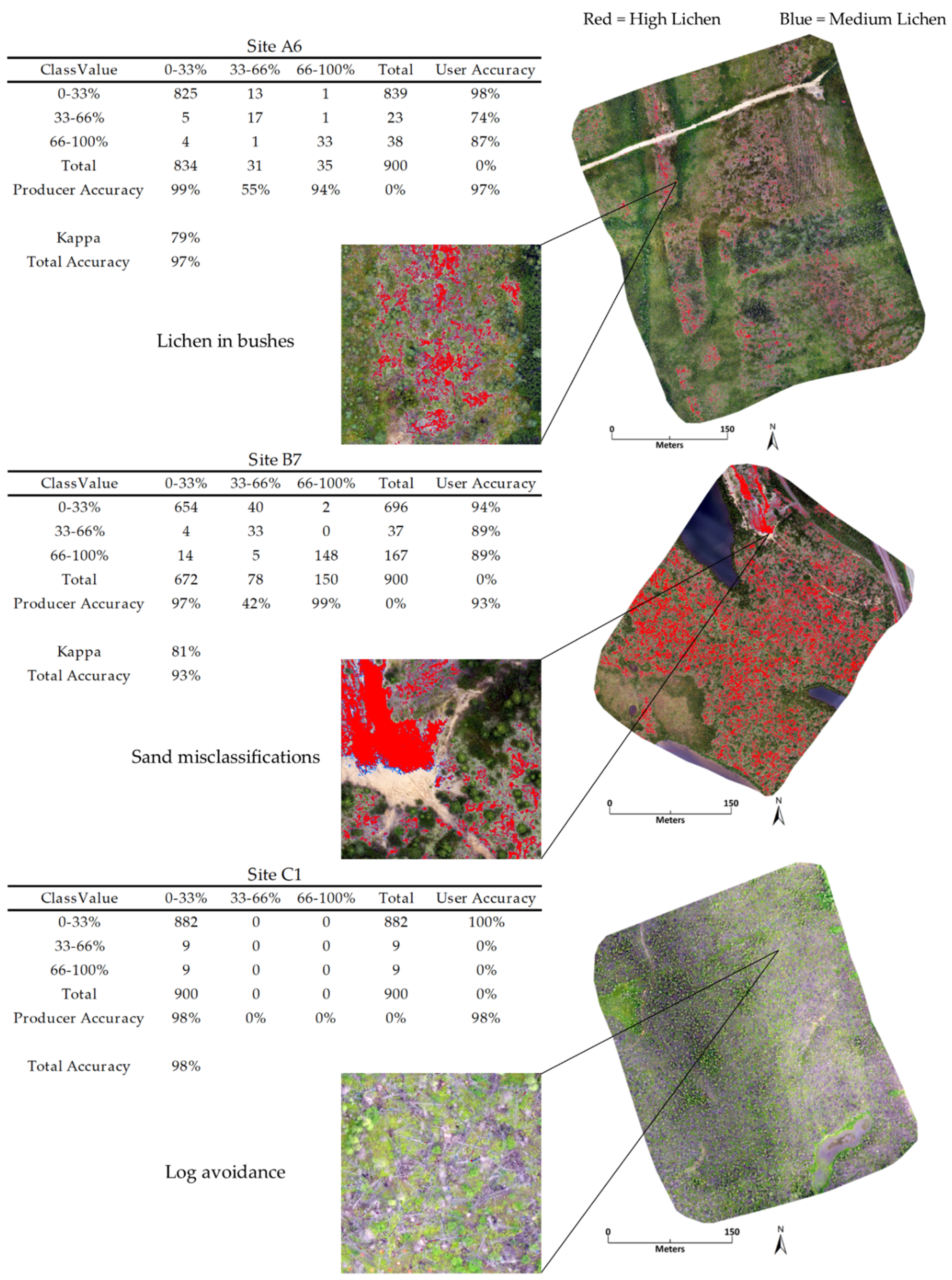
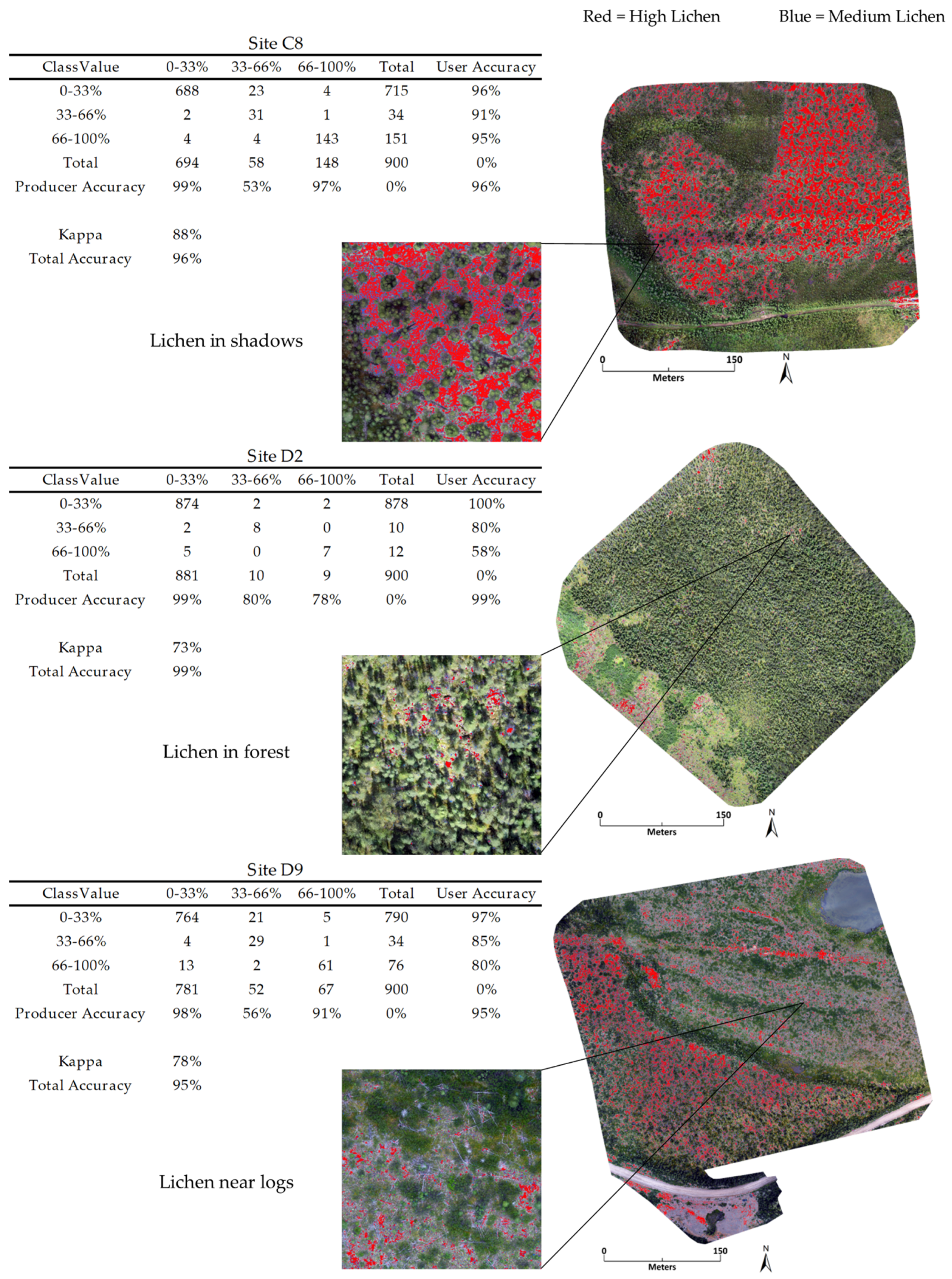
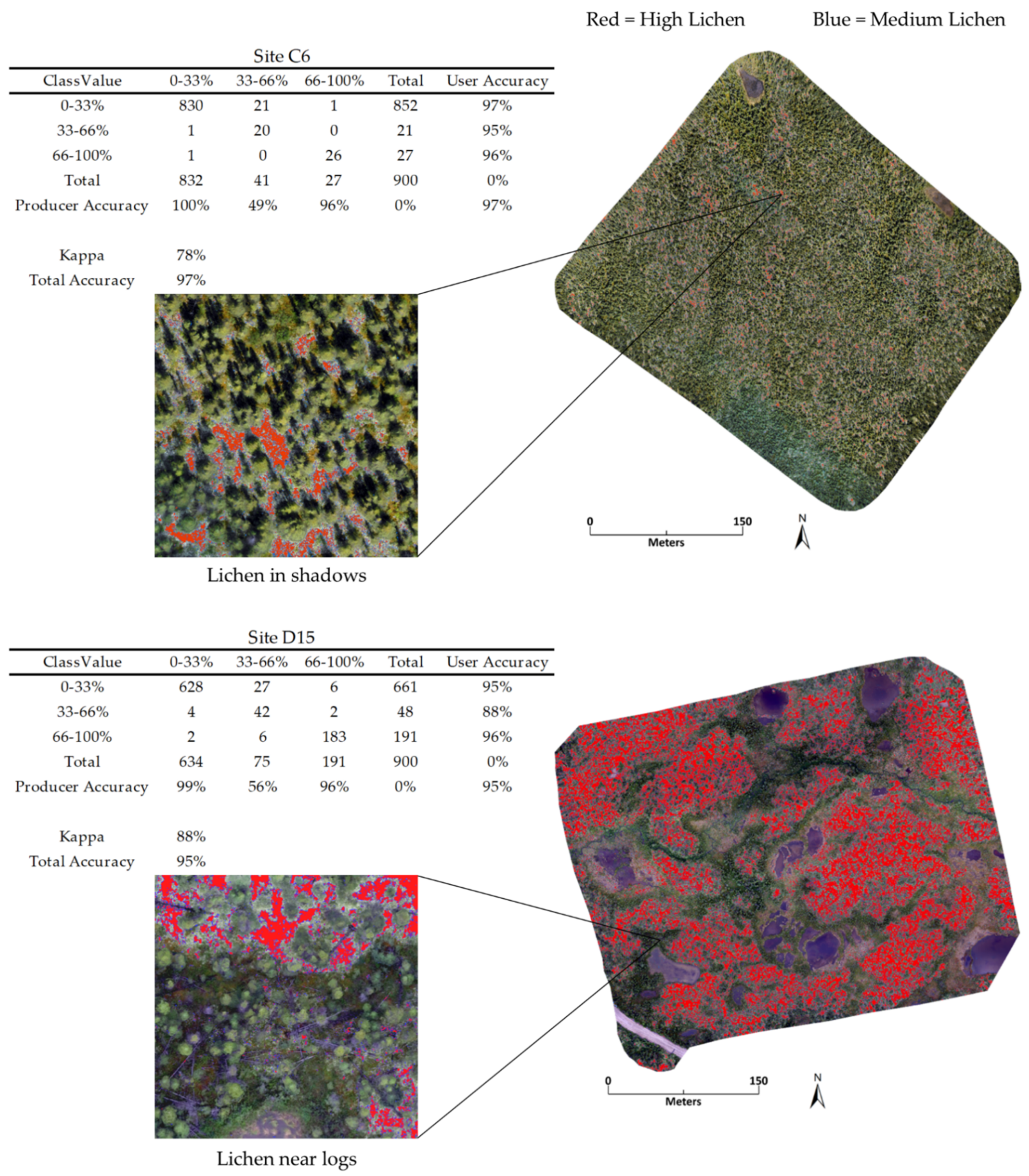
3.2. Manual Point Accuracy Assessment

After processing the eight prediction mosaics using the UAV LiCNN, a manual point accuracy assessment was conducted. For each prediction orthomosaic, we generated 900 sample points using the random stratified method in ArcMap v10.8, where points were randomly distributed within each class and each class had a number of points proportional to its area. The points were manually checked to determine if they accurately represented the three classes. Site C1 is a recently disturbed site containing no lichen due to a recent burn in 2013. This site was included to determine whether the UAV LiCNN is effective at avoiding misclassifications where there are bright logs. Since it has no lichen, it was considered an outlier and excluded from the kappa calculations, overall average accuracies, and overall average kappa.

The manual point accuracy assessment showed that the UAV LiCNN effectively classified pixels, with an average total accuracy of 95.94%. Interrater reliability, an agreement measurement between the expected and observed accuracy, was calculated with an average kappa 80.79%, showing a strong level of agreement [34]. User accuracy, the probability that a predicted value is correct, and producer accuracy, the probability that a value in a class was correctly classified, were calculated for the three classes. The UAV LiCNN is accurate at classifying high lichen pixels, with an average producer and user accuracy of 92.93% and 85.84%, respectively (

Table 2. Summary table outlining the average manual point accuracies per class across seven UAV orthomosaics.

Class	Mean User Accuracy	Mean Producer Accuracy
Low	96.74%	98.75%
Medium	86.04%	55.88%
High	85.84%	92.93%

). Part of the reason for the lower user accuracy can be attributed to the misclassified logs and other ground covers which were not truly lichen. The medium lichen class had an average producer accuracy of 55.88% and a higher user accuracy of 86.04%. The primary reason for the lower producer error in this class can be attributed to the large portion of the low-class pixels truly being medium-class lichen. The low class had the highest average accuracy across all sites, with an average user and producer accuracy of 96.74% and 98.75%, respectively. Figure 6 displays the confusion matrices for Site C6 and Site D15, along with a close-up and map of the orthomosaic composite. Sites C6 and D15 were selected for Figure 6 because they had varying terrain, lighting, and different amounts of lichen. In addition, these orthomosaics highlighted issues with classifying lichen in shadows and lichen near logs.

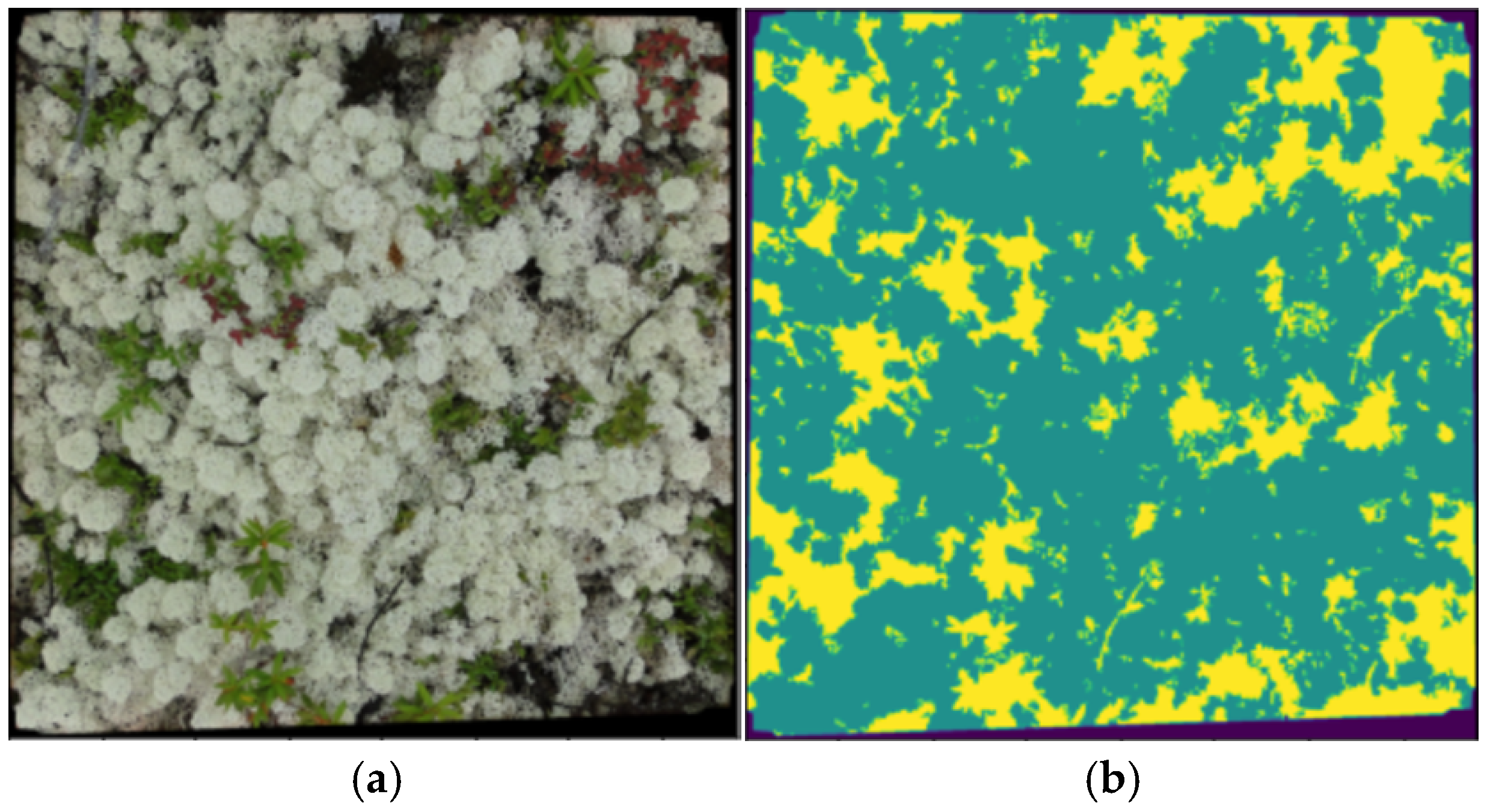
3.3. UAV LiCNN Microplot Prediction and Ground Truth Comparison

The purpose of this accuracy assessment was to determine if there was agreement between the validated lichen percentage of the vegetation microplots and the UAV LiCNN plot prediction values. The lower resolution and motion blurring in the UAV orthomosaic resulted in a significant number of mixed pixels between the orange vegetation microplot frame and the surroundings. Figure 7 highlights the blurring of the vegetation microplot, displaying Site D15 microplot 9 in the UAV orthomosaic and the ground photo. The blurring of the orange pixels displayed in the UAV orthomosaic was caused by the lower resolution (2 cm) than the ground photograph and the motion of the UAV in flight. All orange pixels were avoided when tracing the vegetation microplots for this accuracy assessment. However, this inherently caused significant distortions between the true vegetation microplot lichen % and what could be detected in the orthomosaics.

This accuracy assessment consisted of the 77 vegetation microplots which were visible in the UAV orthomosaics and had respective ground photographs. Vegetation microplots obstructed by trees in the UAV orthomosaic were excluded from this assessment. When comparing the validation data and the UAV LiCNN values, it seems as though the UAV LiCNN underpredicted the lichen in the vegetation microplots. Due to the shape of the data in the scatterplot and our perceived relationship between the values, we decided that a logarithmic regression would best fit the natural pattern in the data given. We achieved an R² of 0.6910 using a two-parameter logarithmic regression. Figure 8 is a graphical comparison of average lichen percentage in the 77 vegetation microplot with the UAV LiCNN predicted values and the logarithmic regression.

4. Discussion

In this study, we described a new methodology for classifying lichen in UAV ortho-imagery using ground photo image composites and a neural network. Our results from testing this methodology on eight UAV orthomosaics representing different ground and lighting conditions showed an overall accuracy of 95.94%. The UAV LiCNN tended to underestimate lichen ground cover in the ‘medium’ class but was highly accurate in estimating low and high coverages. Sticks avoided in the ground photo composites were similar to the logs avoided in the UAV predicted layers. Through testing the UAV LiCNN on a variety of orthomosaics consisting of different landscapes and lighting, we see potential for using this method to classify other types of vegetation or lichen in different regions. The UAV LiCNN performs best on the UAV orthomosaics where there are large lichen patches and few objects having similar RGB values, such as sand or bright logs. A limiting factor to scaling lichen mapping, as highlighted by Jozdani et al., is the lack of diversity in the small training data compared to the larger imagery [15]. Due to the larger extent of the UAV orthomosaics compared to the ground photographs, there are more opportunities for misclassifications of land covers that were not included during neural network training.

The UAV LiCNN seemed to overestimate high lichen in spectrally similar objects, such as the misclassifications of lichen as sand in Site B7, and bright logs in Site C1 and Site D15. None of the training data contained sand, and few of the ground photographs contained bright sticks. Lichen can be found in open clearings and interspersed between trees. Whereas some of the vegetation microplot training photographs had shadows in them, they were not of the same intensity as some of the shadows in Sites C6 and D2. Therefore, we believe that future improvements in UAV HDR cameras or shadow correction could improve classification results.

Another limitation to this study stems from the use of only three spectral bands when using RGB images. In some cases, RGB sensors can be sufficient, such as wetland ecotypes segmentation and wetland delineation [11,17]. However, RGB sensors can fail to provide the necessary data when target objects are spectrally similar to non-target objects across the visible wavelengths, for example, in the case between lichen and bright logs. Lichen reflects more near-infrared radiation (NIR) than non-living features such as sand or logs, and this could be useful for improving differentiation [1]. Whereas UAVs with the NIR band are common for vegetation surveys, high-resolution multispectral handheld cameras that include all three visible bands and the NIR band for ground photographs are uncommon and expensive. Since mosaicking is required for UAV datasets, having the RGB and NIR bands on different cameras is not as much of an issue as individual microplot photographs would be if they came from two different cameras. Thus, implementing a multispectral UAV LiCNN with NIR could be costly.

5. Conclusions

This study demonstrated that a neural network trained on ground photos could classify lichen cover percentages in UAV orthomosaics with high accuracy. Given true masks and high-resolution photographs of vegetation microplots, an UAV LiCNN would be an effective method of classifying lichen in UAV orthomosaics. This AI model is efficient to train and apply to larger orthomosaics. Our results suggest that spectral, surface texture, and spatial patterns detected in ground photographs can be recognized in UAV orthomosaics by the UAV LiCNN, enhancing the classification capabilities of spectrally similar pixels to lichen. In our work, the UAV LiCNN was able to detect high lichen cover (66–100%), with high user and producer accuracies of 85.84% and 92.93%, respectively. In addition, the vegetation microplot accuracy assessment showed that there was agreement between the true vegetation microplot lichen percentage and the UAV LiCNN predicted lichen percentage (R² of 0.6910). We expect that using RGB and NIR ground photographs and UAV orthoimages could help improve the differentiation between lichen and other bright surfaces. Greater diversity in vegetation microplot photographs can also increase the robustness of classification results over larger UAV images. In addition, a methodology for correcting tree shadows in UAV orthomosaics would improve the segmentation results of lichen.

The UAV LiCNN and our methodology can enable researchers to classify lichen under comparable conditions in UAV orthomosaics with high accuracy. This can be used for community maps or for EO up-scaling efforts. The limitations of this methodology include potential misclassifications of lichen as other bright surfaces, and dark shadows covering lichen patches. Further research can improve upon our existing methodology for mapping lichen in UAV orthomosaics.

References

1. Fraser, R.H.; Pouliot, D.; van der Sluijs, J. UAV and high resolution satellite mapping of Forage Lichen (Cladonia spp.) in a Rocky Canadian Shield Landscape. Can. J. Remote Sens. 2021, 1–14. [Google Scholar] [CrossRef]
2. Macander, M.J.; Palm, E.C.; Frost, G.V.; Herriges, J.D.; Nelson, P.R.; Roland, C.; Russell, K.L.; Suitor, M.J.; Bentzen, T.W.; Joly, K.; et al. Lichen cover mapping for Caribou ranges in interior Alaska and Yukon. Environ. Res. Lett. 2020, 15, 055001. [Google Scholar] [CrossRef]
3. Schmelzer, I.; Lewis, K.P.; Jacobs, J.D.; McCarthy, S.C. Boreal caribou survival in a warming climate, Labrador, Canada 1996–2014. Glob. Ecol. Conserv. 2020, 23, e01038. [Google Scholar] [CrossRef]
4. Thompson, I.D.; Wiebe, P.A.; Mallon, E.; Rodger, A.R.; Fryxell, J.M.; Baker, J.A.; Reid, D. Factors influencing the seasonal diet selection by woodland caribou (rangifer tarandus tarandus) in boreal forests in Ontario. Can. J. Zool. 2015, 93, 87–98. [Google Scholar] [CrossRef]
5. Théau, J.; Peddle, D.R.; Duguay, C.R. Mapping lichen in a caribou habitat of Northern Quebec, Canada, using an enhancement-classification method and spectral mixture analysis. Remote Sens. Environ. 2005, 94, 232–243. [Google Scholar] [CrossRef]
6. Gunn, A. Rangifer tarandus. IUCN Red List. Threat. Species 2016, e.T29742A22167140. [Google Scholar] [CrossRef]
7. Dengler, J.; Jansen, F.; Glöckler, F.; Peet, R.K.; de Cáceres, M.; Chytrý, M.; Ewald, J.; Oldeland, J.; Lopez-Gonzalez, G.; Finckh, M.; et al. The Global Index of Vegetation-Plot Databases (GIVD): A new resource for vegetation science. J. Veg. Sci. 2011, 22, 582–597. [Google Scholar] [CrossRef]
8. Kentsch, S.; Caceres, M.L.L.; Serrano, D.; Roure, F.; Diez, Y. Computer vision and deep learning techniques for the analysis of drone-acquired forest images, a transfer learning study. Remote Sens. 2020, 12, 1287. [Google Scholar] [CrossRef] [Green Version]
9. Pap, M.; Kiraly, S.; Moljak, S. Investigating the usability of UAV obtained multispectral imagery in tree species segmentation. International Archives of the Photogrammetry. Int. Arch. Photogramm. Remote Sens. Spat. Inf. 2019, 42, 159–165. [Google Scholar] [CrossRef] [Green Version]
10. Chabot, D.; Dillon, C.; Shemrock, A.; Weissflog, N.; Sager, E.P.S. An object-based image analysis workflow for monitoring shallow-water aquatic vegetation in multispectral drone imagery. ISPRS Int. J. Geo-Inf. 2018, 7, 294. [Google Scholar] [CrossRef] [Green Version]
11. Boon, M.A.; Greenfield, R.; Tesfamichael, S. Wetland assessment using unmanned aerial vehicle (UAV) photogrammetry. Int. Arch. Photogramm. Remote Sens. Spat. Inf. 2016, 41, 781–788. [Google Scholar] [CrossRef] [Green Version]
12. Murugan, D.; Garg, A.; Singh, D. Development of an Adaptive Approach for Precision Agriculture Monitoring with Drone and Satellite Data. IEEE J. Sel. Top. Appl. Earth Obs. Remote Sens. 2017, 10, 5322–5328. [Google Scholar] [CrossRef]
13. Alvarez-Taboada, F.; Paredes, C.; Julián-Pelaz, J. Mapping of the invasive species Hakea sericea using Unmanned Aerial Vehicle (UAV) and worldview-2 imagery and an object-oriented approach. Remote Sens. 2017, 9, 913. [Google Scholar] [CrossRef] [Green Version]
14. Campbell, M.J.; Dennison, P.E.; Tune, J.W.; Kannenberg, S.A.; Kerr, K.L.; Codding, B.F.; Anderegg, W.R.L. A multi-sensor, multi-scale approach to mapping tree mortality in woodland ecosystems. Remote Sens. Environ. 2020, 245, 111853. [Google Scholar] [CrossRef]
15. Jozdani, S.; Chen, D.; Chen, W.; Leblanc, S.G.; Prévost, C.; Lovitt, J.; He, L.; Johnson, B.A. Leveraging Deep Neural Networks to Map Caribou Lichen in High-Resolution Satellite Images Based on a Small-Scale, Noisy UAV-Derived Map. Remote Sens. 2021, 13, 2658. [Google Scholar] [CrossRef]
16. Zhao, T.; Yang, Y.; Niu, H.; Chen, Y.; Wang, D. Comparing U-Net convolutional networks with fully convolutional networks in the performances of pomegranate tree canopy segmentation. Multispectral Hyperspectral Ultraspectral Remote Sens. Technol. Tech. Appl. 2018, 64. [Google Scholar] [CrossRef]
17. Bhatnagar, S.; Gill, L.; Ghosh, B. Drone image segmentation using machine and deep learning for mapping raised bog vegetation communities. Remote Sens. 2020, 12, 2602. [Google Scholar] [CrossRef]
18. Long, J.; Shelhamer, E.; Darrell, T. Fully convolutional networks for semantic segmentation. In Proceedings of the 2015 IEEE Conference on Computer Vision and Pattern Recognition (CVPR) 2015, Boston, MA, USA, 7–12 June 2015. [Google Scholar] [CrossRef] [Green Version]
19. Noh, H.; Hong, S.; Han, B. Learning deconvolution network for semantic segmentation. In Proceedings of the 2015 IEEE International Conference on Computer Vision (ICCV) 2015, Santiago, Chile, 7–13 December 2015. [Google Scholar] [CrossRef] [Green Version]
20. Shi, Q.; Liu, M.; Li, S.; Liu, X.; Wang, F.; Zhang, L. A deeply supervised attention metric-based network and an open aerial image dataset for remote sensing change detection. IEEE Trans. Geosci. Remote Sens. 2021, 1–16. [Google Scholar] [CrossRef]
21. Luo, F.; Zhang, L.; Du, B.; Zhang, L. Dimensionality Reduction with Enhanced Hybrid-Graph Discriminant Learning for Hyperspectral Image Classification. IEEE Trans. Geosci. Remote Sens. 2020, 58, 5336–5353. [Google Scholar] [CrossRef]
22. Ronneberger, O.; Fischer, T.B.P. U-Net: Convolutional Networks for Biomedical Image Segmentation. Lect. Notes Comput. Sci. 2015, 9, 234–241. [Google Scholar] [CrossRef] [Green Version]
23. Abrams, J.F.; Vashishtha, A.; Wong, S.T.; Nguyen, A.; Mohamed, A.; Wieser, S.; Kuijper, A.; Wilting, A.; Mukhopadhyay, A. Habitat-Net: Segmentation of habitat images using deep learning. Ecol. Inform. 2019, 51, 121–128. [Google Scholar] [CrossRef]
24. Tang, H.; Wang, B.; Chen, X. Deep learning techniques for automatic butterfly segmentation in ecological images. Comput. Electron. Agric. 2020, 178, 105739. [Google Scholar] [CrossRef]
25. Jo, H.J.; Na, Y.-H.; Song, J.-B. Data augmentation using synthesized images for object detection. In Proceedings of the 2017 17th International Conference on Control, Automation and Systems (ICCAS) 2017, Jeju, Korea, 18–21 October 2017. [Google Scholar] [CrossRef]
26. Lovitt, J.; Richardson, G.; Rajaratnam, K.; Chen, W.; Leblanc, S.G.; He, L.; Nielsen, S.E.; Hillman, A.; Schmelzer, I.; Arsenault, A. Using AI to estimate caribou lichen ground cover from field-level digital photographs in support of EO-based regional mapping. Remote Sens. 2021, in press. [Google Scholar]
27. He, L.; Chen, W.; Leblanc, S.G.; Lovitt, J.; Arsenault, A.; Schmelzer, I.; Fraser, R.H.; Sun, L.; Prévost, C.R.; White, H.P.; et al. Integration of multi-scale remote sensing data in reindeer lichen fractional cover mapping in Eastern Canada. Remote Sens. Environ. 2021, in press. [Google Scholar]
28. Miranda, B.R.; Sturtevant, B.R.; Schmelzer, I.; Doyon, F.; Wolter, P. Vegetation recovery following fire and harvest disturbance in central Labrador—a landscape perspective. Can. J. For. Res. 2016, 46, 1009–1018. [Google Scholar] [CrossRef] [Green Version]
29. Schmelzer, I. CFS Lichen Mapping 2019. (J. Lovitt, Interviewer).
30. Leblanc, S.G. Off-the-shelf Unmanned Aerial Vehicles for 3D Vegetation mapping. Geomat. Can. 2020, 57, 28. [Google Scholar] [CrossRef]
31. Fernades, R.; Prevost, C.; Canisius, F.; Leblanc, S.G.; Maloley, M.; Oakes, S.; Holman, K.; Knudby, A. Monitoring snow depth change across a range of landscapes with ephemeral snowpacks using structure from motion applied to lightweight unmanned aerial vehicle videos. Cryosphere 2018, 12, 3535–3550. [Google Scholar] [CrossRef] [Green Version]
32. Nordberg, M.L.; Allard, A. A remote sensing methodology for monitoring lichen cover. Can. J. Remote Sens. 2002, 28, 262–274. [Google Scholar] [CrossRef]
33. Bauerle, A.; van Onzenoodt, C.; Ropinski, T. Net2Vis—a visual grammar for automatically generating Publication-Tailored Cnn Architecture Visualizations. IEEE Trans. Vis. Comput. Graph. 2021, 27, 2980–2991. [Google Scholar] [CrossRef] [PubMed]
34. McHugh, M.L. Lessons in biostatistics interrater reliability: The kappa statistic. Biochem. Med. 2012, 22, 276–282. [Google Scholar] [CrossRef]
Figure 1. The ground photo (a) and DPC mask (b) for Site D15 microplot 9. The classes for the mask on the right are green for lichen, yellow for not lichen, and purple for border.
Drones 05 00099 g001
Figure 2. Creation of the training mosaics. Ground photographs were resized, cropped, and resized to 80 × 80 px before being stitched into mosaics. Input masks were resized, cropped, and resized to 80 × 80 px before being separated into three classes. The reclassified masks, with red as high lichen, blue as medium lichen, and green as none to low lichen, were then stitched into mosaics representative of the respective ground photo mosaics.
Drones 05 00099 g002
Figure 3. Crop and resize data augmentations. A diagram outlining the crop and resize data augmentations in the UAV LiCNN training.
Drones 05 00099 g003
Figure 4. UAV LiCNN Neural Network Model. A visualization of the UAV LiCNN architecture showing the input dimensions and the model layers.
Drones 05 00099 g004
Figure 5. UAV LiCNN prediction script. A workflow diagram outlining the UAV LiCNN prediction script, where the input orthomosaics are broken up into tiles, passed through a trained neural network model. Then, the prediction tiles are stitched together to make an output mosaic.
Drones 05 00099 g005
Figure 6. UAV LiCNN manual point accuracy assessment. A descriptive graphic with confusion matrices, highlighted closeups, and the prediction mosaic transposed on the UAV orthomosaics for sites C6 and D15. All other orthomosaics and confusion matrices can be found in Appendix A Figure A1 and Figure A2.
Drones 05 00099 g006
Figure 7. Comparison of Site D15 microplot 9 in the UAV orthomosaic (a) with the ground photo (b).
Drones 05 00099 g007
Figure 8. Scatterplot with two parameter logarithmic regression comparing the true percentage of lichen in the vegetation microplots with the predicted values from the UAV LiCNN.
Drones 05 00099 g008