
Thermal Sensor Calibration for Unmanned Aerial Systems Using an External Heated Shutter

 , , ,
, , ,  and
and 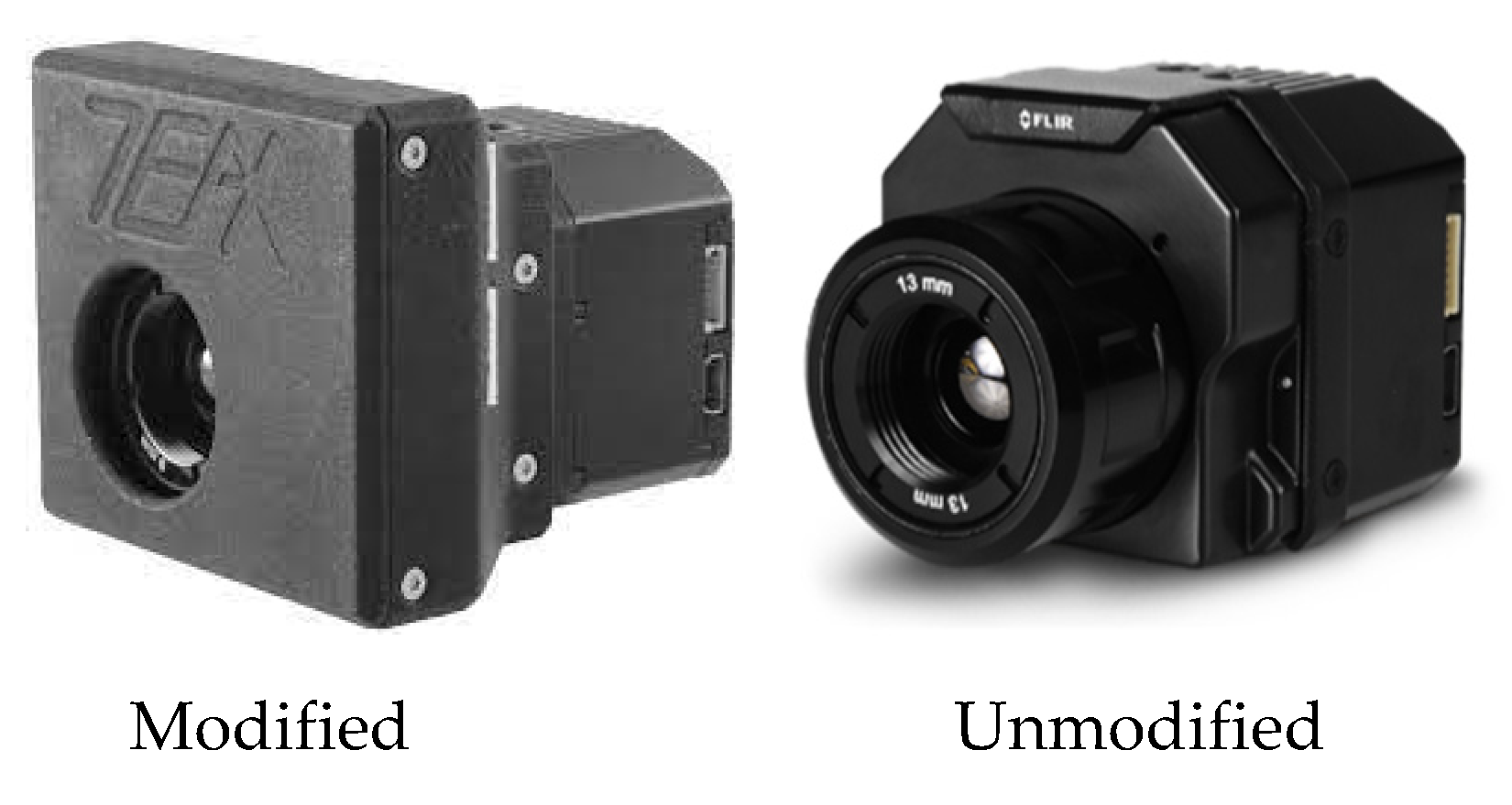
Abstract
:1. Introduction
1.1. Thermal Sensors and UAS
1.2. Previous Studies Addressing Thermal Sensor Drift
1.3. This Study
2. Data and Methodology
2.1. Laboratory Tests and Equipment
2.1.1. Thermal Sensor and Thermal Capture Calibrator
2.1.2. Laboratory Configuration
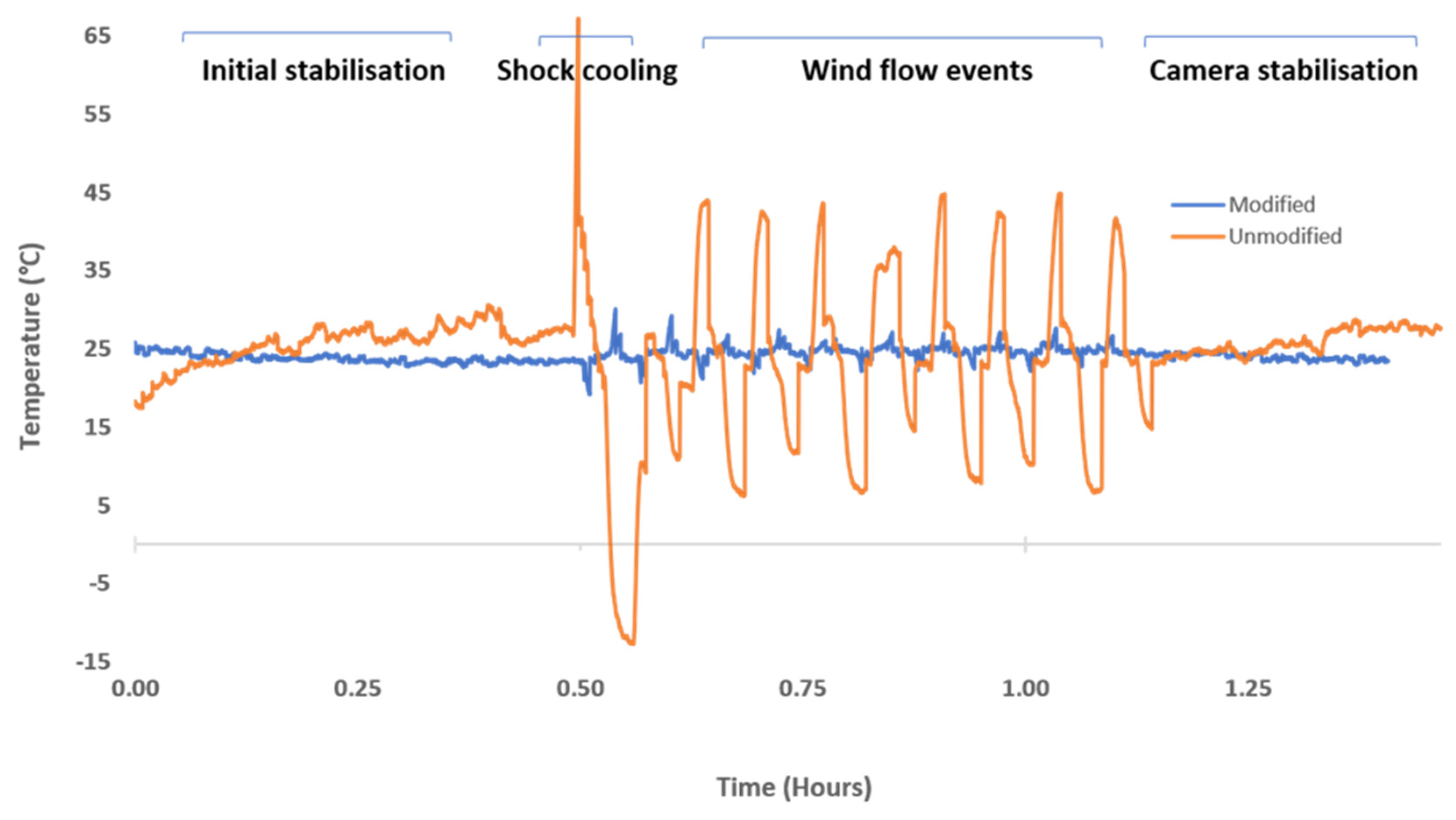
2.1.3. Simulating Operational Wind Conditions
2.2. Field Tests
2.2.1. UAS and Flight Planning
2.2.2. Field Operations
2.3. Image Processing
2.3.1. Blackbody Imaging
2.3.2. Vignetting Filter
2.3.3. Orthomosaics and Orthophotos
2.3.4. Orthophoto Image Calculations
3. Results
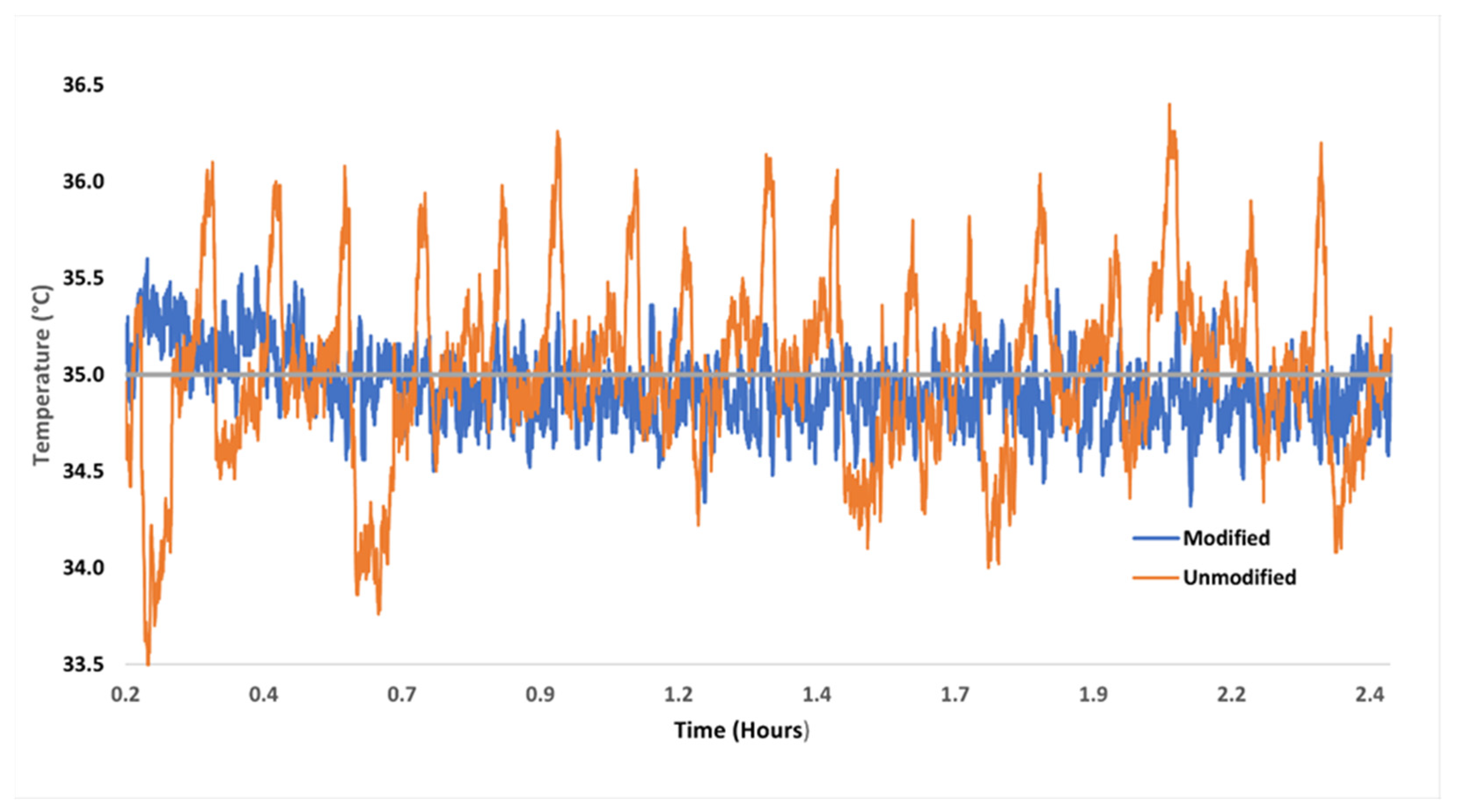
3.1. Laboratory-Based Experiment
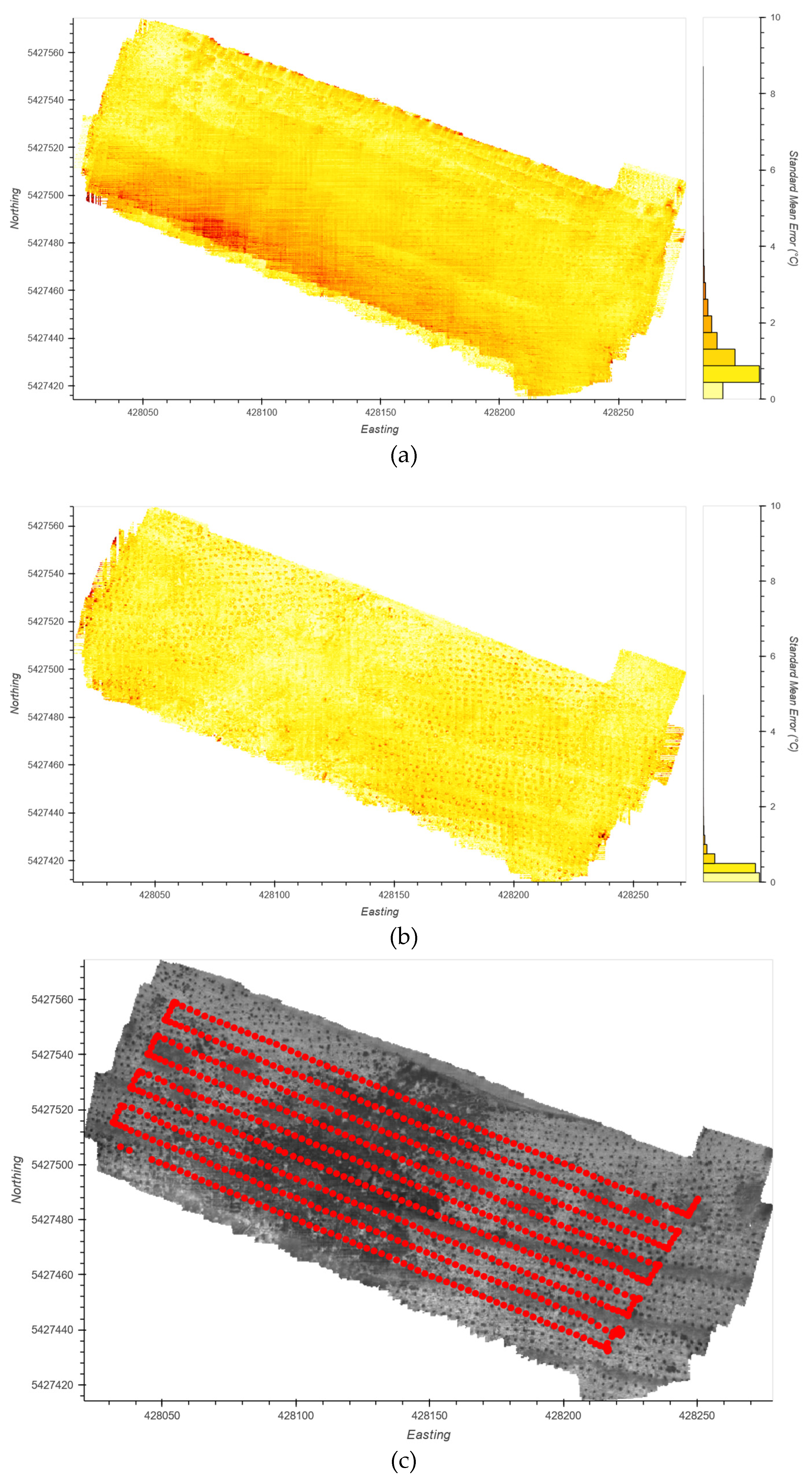
3.2. Field Based Experimentation
4. Discussion
4.1. Laboratory Calibration
4.2. Field Operation
4.3. Operational Recommendations
- Upon commencement of a mapping mission, fly for 2–3 min at a speed of 4 m/s prior to data collection to allow the sensor to be ‘shock cooled’ to ambient conditions;
- Although absolute temperature accuracy was not assessed in this study, deployment of thermal calibration targets is recommended at the beginning of the study to initially verify ground temperate. The temperature stabilising benefits of the heated shutter has the potential to reduce of remove the requirement for ground calibration targets; however, this relies on further testing and validation of the absolute temperature measurements made by the modified camera;
- Fly mapping mission with high overlap (≥80%) to account for reduced thermal observations during the flat field correction;
- Post-processing of extra images collected by the sensor should be removed to ensure the first image used in the model is the first image of the flight line, as the largest pixel DN value discrepancy occurs within the first 2–3 min of sensor operation during the ‘shock cooling’ event;
- We show here that the use of a heated shutter, or some form of insulation around the sensor, should be considered to help alleviate ‘shock cooling’ events.
5. Conclusions
Author Contributions
Funding
Data Availability Statement
Acknowledgments
Conflicts of Interest
References
- Gómez-Candón, D.; Virlet, N.; Sylvain, L.; Jolivot, A.; Regnard, J.L. Field phenotyping of water stress at tree scale by UAV-sensed imagery: New insights for thermal acquisition and calibration. Precis. Agric. 2016, 17, 786–800. [Google Scholar] [CrossRef]
- Hoffmann, H.; Jensen, R.; Thomsen, A.; Nieto, H.; Rasmussen, J.; Friborg, T. Crop water stress maps for an entire growing season from visible and thermal UAV imagery. Biogeosciences 2016, 13, 6545–6563. [Google Scholar] [CrossRef] [Green Version]
- Smigaj, M.; Gaulton, R.; Suarez, J.C.; Barr, S.L. Use of miniature thermal cameras for detection of physiological stress in conifers. Remote Sens. 2017, 9, 957. [Google Scholar] [CrossRef] [Green Version]
- Zarco-Tejada, P.J.; González-Dugo, V.; Berni, J.A. Fluorescence, temperature and narrow-band indices acquired from a UAV platform for water stress detection using a micro-hyperspectral imager and a thermal camera. Remote Sens. Environ. 2012, 117, 322–337. [Google Scholar] [CrossRef]
- Calderón, R.; Navas-Cortés, J.A.; Lucena, C.; Zarco-Tejada, P.J. High-resolution airborne hyperspectral and thermal imagery for early detection of Verticillium wilt of olive using fluorescence, temperature and narrow-band spectral indices. Remote Sens. Environ. 2013, 139, 231–245. [Google Scholar] [CrossRef]
- Baratchi, M.; Meratnia, N.; Havinga, P.J.; Skidmore, A.K.; Toxopeus, B.A. Sensing solutions for collecting spatio-temporal data for wildlife monitoring applications: A review. Sensors 2013, 13, 6054–6088. [Google Scholar] [CrossRef] [Green Version]
- Gonzalez-Dugo, V.; Zarco-Tejada, P.; Nicolás, E.; Nortes, P.A.; Alarcón, J.; Intrigliolo, D.S.; Fereres, E. Using high resolution UAV thermal imagery to assess the variability in the water status of five fruit tree species within a commercial orchard. Precis. Agric. 2013, 14, 660–678. [Google Scholar] [CrossRef]
- Brunton, E.A.; Leon, J.X.; Burnett, S.E. Evaluating the efficacy and optimal deployment of thermal infrared and true-colour imaging when using drones for monitoring kangaroos. Drones 2020, 4, 20. [Google Scholar] [CrossRef]
- Brenner, C.; Zeeman, M.; Bernhardt, M.; Schulz, K. Estimation of evapotranspiration of temperate grassland based on high-resolution thermal and visible range imagery from unmanned aerial systems. Int. J. Remote Sens. 2018, 39, 5141–5174. [Google Scholar] [CrossRef] [PubMed] [Green Version]
- Lhoest, S.; Linchant, J.; Quevauvillers, S.; Vermeulen, C.; Lejeune, P. How many hippos (HOMHIP): Algorithm for automatic counts of animals with infra-red thermal imagery from UAV. Int. Arch. Photogramm. Remote Sens. Spat. Inf. Sci. 2015, 40, 355–362. [Google Scholar] [CrossRef] [Green Version]
- Seymour, A.C.; Dale, J.; Hammill, M.; Halpin, P.N.; Johnston, D.W. Automated detection and enumeration of marine wildlife using unmanned aircraft systems (UAS) and thermal imagery. Sci. Rep. 2017, 7, 45127. [Google Scholar] [CrossRef] [Green Version]
- McCarthy, E.D.; Martin, J.M.; Boer, M.M.; Welbergen, J.A. Drone-based thermal remote sensing provides an effective new tool for monitoring the abundance of roosting fruit bats. Remote Sens. Ecol. Conserv. 2021, 7, 461–474. [Google Scholar] [CrossRef]
- Budzier, H.; Gerlach, G. Calibration of uncooled thermal infrared cameras. J. Sens. Sens. Syst. 2015, 4, 187–197. [Google Scholar] [CrossRef] [Green Version]
- Mesas-Carrascosa, F.-J.; Pérez-Porras, F.; De Larriva, J.E.M.; Mena- Frau, C.; Agüera-Vega, F.; Carvajal-Ramírez, F.; Martínez-Carricondo, P.; García-Ferrer, A. Drift correction of lightweight microbolometer thermal sensors on-board unmanned aerial vehicles. Remote Sens. 2018, 10, 615. [Google Scholar] [CrossRef] [Green Version]
- Flir. Thermal Drone Resources & Training. Available online: https://www.flir.com.au/support-center/training/suas/ (accessed on 3 February 2021).
- Olbrycht, R.; Więcek, B. New approach to thermal drift correction in microbolometer thermal cameras. Quant. Infrared Thermogr. J. 2015, 12, 184–195. [Google Scholar] [CrossRef]
- Aragon, B.; Johansen, K.; Parkes, S.; Malbeteau, Y.; Al-Mashharawi, S.; Al-Amoudi, T.; Andrade, C.F.; Turner, D.; Lucieer, A.; McCabe, M.F. A calibration procedure for field and UAV-based uncooled thermal infrared instruments. Sensors 2020, 20, 3316. [Google Scholar] [CrossRef] [PubMed]
- Tempelhahn, A.; Budzier, H.; Krause, V.; Gerlach, G. Shutter-less calibration of uncooled infrared cameras. J. Sens. Sens. Syst. 2016, 5, 9–16. [Google Scholar] [CrossRef] [Green Version]
- Flir Tech Note. Available online: https://www.flir.com/globalassets/guidebooks/suas-radiometric-tech-note-en.pdf (accessed on 11 April 2021).
- Ribeiro-Gomes, K.; Hernández-López, D.; Ortega, J.F.; Ballesteros, R.; Poblete, T.; Moreno, M.A. Uncooled thermal camera calibration and optimization of the photogrammetry process for UAV applications in agriculture. Sensors 2017, 17, 2173. [Google Scholar] [CrossRef]
- Maes, W.H.; Huete, A.R.; Steppe, K. Optimizing the processing of UAV-based thermal imagery. Remote Sens. 2017, 9, 476. [Google Scholar] [CrossRef] [Green Version]
- Torres-Rua, A. Vicarious calibration of sUAS microbolometer temperature imagery for estimation of radiometric land surface temperature. Sensors 2017, 17, 1499. [Google Scholar] [CrossRef] [PubMed] [Green Version]
- Pestana, S.; Chickadel, C.C.; Harpold, A.; Kostadinov, T.S.; Pai, H.; Tyler, S.; Webster, C.; Lundquist, J.D. Bias correction of airborne thermal infrared observations over forests using melting snow. Water Resour. Res. 2019, 55, 11331–11343. [Google Scholar] [CrossRef]
- Olbrycht, R.; Więcek, B.; De Mey, G. Thermal drift compensation method for microbolometer thermal cameras. Appl. Opt. 2012, 51, 1788–1794. [Google Scholar] [CrossRef]
- TeAX. ThermalCapture Calibrator. Available online: https://thermalcapture.com/thermalcapture-calibrator/ (accessed on 10 February 2021).
- Kelly, J.; Kljun, N.; Olsson, P.-O.; Mihai, L.; Liljeblad, B.; Weslien, P.; Klemedtsson, L.; Eklundh, L. Challenges and best practices for deriving temperature data from an uncalibrated UAV thermal infrared camera. Remote Sens. 2019, 11, 567. [Google Scholar] [CrossRef] [Green Version]
- Acorsi, M.G.; Gimenez, L.M.; Martello, M. Assessing the performance of a low-cost thermal camera in proximal and aerial conditions. Remote Sens. 2020, 12, 3591. [Google Scholar] [CrossRef]
- Ludovisi, R.; Tauro, F.; Salvati, R.; Khoury, S.; Mugnozza, G.S.; Harfouche, A. UAV-based thermal imaging for high-throughput field phenotyping of black poplar response to drought. Front. Plant Sci. 2017, 8, 1681. [Google Scholar] [CrossRef] [PubMed]
- Testi, L.; Goldhamer, D.; Iniesta, F.; Salinas, M. Crop water stress index is a sensitive water stress indicator in pistachio trees. Irrig. Sci. 2008, 26, 395–405. [Google Scholar] [CrossRef] [Green Version]
- Wang, D.; Gartung, J. Infrared canopy temperature of early-ripening peach trees under postharvest deficit irrigation. Agric. Water Manag. 2010, 97, 1787–1794. [Google Scholar] [CrossRef]
- Berni, J.; Zarco-Tejada, P.; Suárez, L.; González-Dugo, V.; Fereres, E. Remote sensing of vegetation from UAV platforms using lightweight multispectral and thermal imaging sensors. Int. Arch. Photogramm. Remote Sens. Spat. Inform. Sci. 2009, 38, 6. [Google Scholar]

Publisher’s Note: MDPI stays neutral with regard to jurisdictional claims in published maps and institutional affiliations. |
© 2021 by the authors. Licensee MDPI, Basel, Switzerland. This article is an open access article distributed under the terms and conditions of the Creative Commons Attribution (CC BY) license (https://creativecommons.org/licenses/by/4.0/).
Share and Cite
Virtue, J.; Turner, D.; Williams, G.; Zeliadt, S.; McCabe, M.; Lucieer, A. Thermal Sensor Calibration for Unmanned Aerial Systems Using an External Heated Shutter. Drones 2021, 5, 119. https://doi.org/10.3390/drones5040119
Virtue J, Turner D, Williams G, Zeliadt S, McCabe M, Lucieer A. Thermal Sensor Calibration for Unmanned Aerial Systems Using an External Heated Shutter. Drones. 2021; 5(4):119. https://doi.org/10.3390/drones5040119
Chicago/Turabian StyleVirtue, Jacob, Darren Turner, Guy Williams, Stephanie Zeliadt, Matthew McCabe, and Arko Lucieer. 2021. "Thermal Sensor Calibration for Unmanned Aerial Systems Using an External Heated Shutter" Drones 5, no. 4: 119. https://doi.org/10.3390/drones5040119
APA StyleVirtue, J., Turner, D., Williams, G., Zeliadt, S., McCabe, M., & Lucieer, A. (2021). Thermal Sensor Calibration for Unmanned Aerial Systems Using an External Heated Shutter. Drones, 5(4), 119. https://doi.org/10.3390/drones5040119