Early Detection of Obstacle to Optimize the Robot Path Planning

Abstract

Robot path planning is one of the core issues in robotics and its application. Optimizing the route discovery becomes more important while dealing with the robot-based application. This paper proposes the concept of early detection of the obstacle present in the workspace of the robots. To early detect the obstacle, this paper proposes the concept of a snake algorithm along with the traditional path planning algorithms. The contour detection part is merged with the different path planning algorithms to optimize the robot traversing and benefit it in producing good results. Obstacle-free optimized path is one of the core requirements for robots in any application. With the help of path planning algorithms, robots are enabled to derive those paths in a specific environment. The presence of an obstacle makes it difficult for any path planning algorithms to derive a smooth path. The purpose of using the snake algorithm is to detect an obstacle early. This method not only perceives the obstacle but also catches out the complete boundary of the obstacle, it, thus, provides the details of obstacle coordinates to the path planning algorithm. Conceiving the complete periphery of obstacles can have multiple advantages in many application areas. A*, PRM, RRT, and RRT Smooth algorithms are considered along with the snake algorithm to validate our work in three different experimental scenarios: Maze, Random Obstacles, and Dense case. Path length, Time-taken, and Move count are parameters taken to observe the results. The result obtained using the snake algorithm with four path planning algorithms is analyzed and compared in detail with the core A*, PRM, RRT, and RRTS. Finally, the result obtained using the proposed methodology gives some encouraging results and also predicts the exploration of the robot’s path planning for more applications and fields.

1. Introduction

Path planning is to move smoothly from one point to another without any hitch and hindrance. It is one of the prime facets for mobile robots to find the shortest path or otherwise optimal path. The optimal path in robotics could be the path that reduces the computation time, number of turnings, and the distance between the source and destination. Assume a case where a robot is positioned in a square room, the two endpoints of the diagonal of that square room are the source and destinations point for the robot. It is now required to travel from source point to destination, there are multiple items placed between these two points, and to reach the destination the robot has to avoid those objects placed in its path to avoid any clash. Now it becomes the need of the system to achieve a smooth traversal in minimum time and effort. This problem soils the requirement of planning a path and here comes the role of path planning algorithms. Algorithms for finding the shortest path are not restricted only to robotics but also have a wide range of applications, such as in network routing, vehicular routing, and video games, whereas the definition of an optimal path varies as per the application area. Path planning for robots has two fundamental procedures to be carried out initially: map representation and path planning algorithms.

The first step in doing path planning for robots requires an environmental set-up or a map of the environment. This environment is called the workspace or configuration space for robots. After finalizing the environment, the robot is then positioned on the map and is assumed to be aware of its location on the map. It, thus, localizes itself and is capable of avoiding the obstacle coming on its way. Selection of map representation is also one of the critical tasks as it should resemble the appropriate application. One more thing which needs to pay attention to is that the robot should be a point-sized robot, as it would not be feasible every time to test algorithms on physical robots. So before actually taking on the algorithms, these two things should be obvious, i.e., map representation resembling the application area and point-sized robots. In Map representation, first of all, it is required to delineate the environment in the computer. This environment constitutes the configuration space for robots. There are two approaches to do that, discrete and continuous approximations. The map taken for testing is divided into equal parts or in different sizes (grids) in the discrete approximation technique.

The overall map representation for computation is classified into two categories discrete maps and continuous maps. The map taken for the experiment is mostly a continuous map that represents a topological nature, while in the case of graph representation, discrete maps are preferred. It comprises various nodes. Each chunk of plans corresponds to a vertex and is connected by edges so that a robot can smoothly traverse from one node to the other. For instance, an image taken nearby or from the surrounding is generally a topological map, the intersection possessed by the map are called vertices and the roads in it are the edges. A graph is usually stored in the computer in the form of an adjacency list or incidence matrix. In any continuous image, the paths are traced and represented as the sequencing of real numbers. The continuous image requires the complete detail of internal and external boundaries and are represented in the form of a polygon. That is why discrete maps are predominantly used in robotics. Grid map is mostly used by the researcher for their experiment. In the grid map, the complete scenario is divided into squares of a specific size (for example 1 cm × 1 cm) the obstacles are also marked in it. Probabilistic maps are another version that marks the presence of obstacles based on probability; they become helpful in many situations where the robot is unaware of its position and the environment. The reason to use topological maps is that the grid maps consume a lot of memory power and processing time to traverse a large ’n’ number of vertices present in it.

Once the environment has been defined, the role of path planning algorithms begins. The word path planning has many distinct names in different study domains, such as motion planning, the navigation problem, the piano mover’s problem, and many more. One of the most crucial aspects to consider is identifying the obstacles on the road. The path planning algorithm’s performance is determined by the location and type of obstacle. When evaluating the path in any given environment, multiple elements are taken into account. In this research, we looked at three parameters: path length, number of moves, and computation time. Four algorithms, namely A*, PRM, RRT, and RRT Smooth, are tested on three different scenarios for pathfinding, coupled with the Snake Algorithm. The Snake Algorithm is used first to discover the obstacles’ locations, and then the specific algorithm is used to find the pathways. The subsection that follows provides a full overview of the overall document as well as insight into the work done for path planning. The study suggests combining a snake algorithm with a path planning system [1].

Path Planning

After setting up the environment for the path planning algorithm to test, The next step to pursue the objective is to indulge in the concept of path planning. Understanding the concept of path planning requires getting familiar with some basic notions related to path planning. The first one is the configuration space/workspace, which means the platform or the environmental set-up where the experiments need to be performed, broadly it may either be 2D/3D Environments. To represent 2D, we require three parameters, $(x,y,\theta )$, whereas, in the 3D environment, it requires six parameters, three for translation and three for defining Euler angles to describe the configuration space. In this article, we have taken three different scenarios based on a 2D environment, namely Maze, random obstacles, and dense case scenarios to perform our experiment. The next important notion is the type of robot considered for work, and it may be a point/zero-sized robot, 2D shape robot, and in some cases, 3D also. Here in this article, we have taken point-sized robots for our experimentation. The next most crucial notion is the different parts of the workspace. Here workspace means the complete environmental set-up where the experiment is carried out. It comprises free space, which means the space where traversal is possible and preferred. Complex space is the area that needs to be discarded and skipped as this is the space occupied by the obstacle present in the workspace. Moreover, in the last, the selection of two points/coordinates between the path is to be found. They are called the source point and destination point [2].

2. Background and Related Work

A hefty amount of work is present to date in the area of path planning. As discussed in the above section, there are multiple parameters and scenarios present in the literature, which displays the right amount of work. In the above section, we mentioned about 2D/3D environment, but here the entire classification and literature part is primarily based on 2D classification. Initially, the entire work can be broadly classified based on an environment that is either constant or dynamic. The term constant and dynamic denotes the nature of the obstacle present in the environment [3]. This section lists out all the notable path planning techniques citing all the relevant work done to date [4]. Some of the notable contributions in this field are: Evolutionary Algorithm [5], Hybrid Algorithm [6], Bee Colony Optimization [7], PSO [8], Bacteria Foraging [9], ACO [10], Artificial Neural Network [11], and Fuzzy Logic [11].

The path planning problem is a well-known NP-hardness [12]. The work carried out over the years for solving the path planning problems can be understood by putting down the two perspectives; the first one is to classify the environments where the problem is being placed and solved, and the second perspective is how it has been solved. As mentioned in the previous section about 2D/3D environment, the first classification can be made based on this point whether the problem lies in a Two-Dimensional or Three-Dimensional zone, The next classification is about whether the problem is global or local. Global path planning requires a map of the complete environment to trace the best route in it. It requires a complete map before the start. To minimize the workload of global path planning, it is split into local waypoints. In local path planning, the map is reduced to the nearby robots for path planning to accomplish the nearest checkpoints [13]. The next classification is about completeness which means the desired output is exact or it is nearby the exact solution, several bio-inspired algorithms with their many amendments fall in this classification  [14].

Evolution means understanding the progress made to date from the point where it started. Starting from the concept of potential field (1979) [15], Roadmap Cell Decomposition (1987) to solve path planning problems to the various techniques of bio-inspired and nature inspire algorithms in recent days [16].

Table 1. Comparison of Different Algorithms with coordinates positions considered in the Experiment.

Algorithm	Size	Start Position	Goal Position
A*	200 × 200	$s_x$ = 93, $s_y$ = 9	$g_x$ = 125, $g_y$ = 138
PRM	200 × 200	$s_x$ = 93, $s_y$ = 9	$g_x$ = 125, $g_y$ = 138
RRT	200 × 200	$s_x$ = 23, $s_y$ = 31	$g_x$ = 178, $g_y$ = 152
RRT S	200 × 200	$s_x$ = 23, $s_y$ = 31	$g_x$ = 178, $g_y$ = 152

present the evolutionary approach used to solve path planning problems over the years. To make it more understandable, we have divided it into classical and heuristic approaches. Classical approaches have the limitation of working in high dimensions and suffer from high complexity. Sometimes it also gets trapped into the local minima which becomes its most significant loophole for its wide acceptability. Some notable algorithms like PRM and RRT have been developed to solve such issues in path planning. Several other concepts, like Genetic algorithms and neural network models, Graph theory-based approach [12] come under the heuristic approach for solving path planning problems. Some of the widely accepted algorithms (R.I. in the table mentions the research impact of that particular technique over the years) there are many more versions of well-known techniques like PRM, RRT, and GA being presented by researchers down the years.

3. Problem Formulation

This section is divided into three subsections to get a clear understanding and perspective of the problems related to path planning for robots. Several algorithms related to path planning were developed and tested in many environments. The measure of Performances (MOP) becomes complicated due to performing in different images, so first, the problem is to have the proper representation of the application scenario and should follow some standards (References Maps). Each application has different operational environments with constraints on the platforms. It is required to have reference test maps to precisely compare the performance with each other. This paper deals with the 2D scenario only, and for that, it has taken three different reference maps for testing the path planning algorithms. Once the standard maps are selected, the next problem is to get an optimized obstacle-free path. The performance of path planning algorithms is greatly affected by the obstacle, thus, affecting the results in many ways. Most of path planning algorithm suggests a different way to deal with the obstacles while traversing for finding paths. They mostly differ in their traversing mechanism and opt for different ways to derive paths. This paper proposes the use of the Snake algorithm for detecting obstacles in advance with its complete periphery; it splits the workspace into two parts, free space and complex space, where free space is the space that is to be traversed by the path planning algorithms and complex space is the space to be voided by the algorithms. Snake Algorithm helps to reduce the traversing space for path planning algorithms. Thus, it helps to improve performance.

3.1. Reference Maps

2D Maps are extensively used in the path planning field, as they can be easily implemented by the image files; several algorithms were developed and tested in many environments. Here, we describe the three reference maps used to test the proposed path planning algorithms. In this particular reference map, the obstacles are fixed in nature. It is a path or collection of paths, typically from a source point to a goal point which has walls as the obstacles. There might be some dead-end; thus, a lot of backtracking ability of the algorithm is required to find a path from the source to the goal node in path planning. Then it is further taken as input to implement A*, PRM, RRT, and RRT Smooth Algorithms. The sample image is presented in the result section, where the proposed algorithm is tested with four algorithms in association with snake algorithms. The second type of map chosen consists of random obstacles; four types of obstacles (circle, square, triangle, and termini shapes) are chosen. This type of map is useful in representing a complex city that consists of 3D buildings and obstacles which need to be scanned for smooth path traversing [17]. This environment may consist of either disjoint obstacles or overlapping obstacles from the above list of obstacles. Then the robot has to calculate the optimal path in the structured environment. The formulated environment consisting of the obstacle from the list is then taken as input for implementing A*, PRM, RRT, and RRT Smooth Algorithms. The third type of map considered is of Dense type. Usually, this type of image is useful for drones or 2/3D hemisphere obstacles that represent radar sites. This environment consists of images that are densely populated that contain color pixels throughout the image. This type of environment may include a picture captured by a camera or by a sensor to locate the optimal path from the source to the destination node. Here, a picture of the NIT Raipur campus has been taken to account for experimentation. After the implementation of a snake algorithm, the output gives a clear specific idea of free space and the area occupied by the obstacles.

3.2. Measure of Performances

Path Length is one of the most important parameters of path planning. It is the summation of variable $lv$ for all the coordinate value pair $(x,y)$ in the final optimal path obtained. The path length is calculated between the source and destination. The algorithm traverses completely the free space based on which it derives the shortest path, which is considered for robots to move from source to destination. The distance of the path is calculated with the help of Euclidian Distance. The distance between two locations in one dimension is defined as the absolute value of the difference between their coordinates in the Euclidean Distance system. In mathematical notation, this is written as $|p_1-q_1|$ where $p_1$, $q_1$ are the first and second coordinates, respectively. This difference is expressed as an absolute value as the distance is typically thought of as having only positive values [18].

$$lv=\sqrt{({(x\left[i\right]-x[i-1])}^2+{(y\left[i\right]-y[i-1])}^2)}$$

(1)

The number of Moves is another important parameter when a robot needs to perform in some uneven planes where the number of moves becomes important to count, it is calculated by the angle between the x-coordinate and the hypotenuse of the final optimal path. This is calculated pixel by pixel, and thus, if any change is detected between the current and previous slope, then the counter is incremented by one [19]. The function $Math.arccosine\left(\right)$ is used to calculate and count the number of moves taken by the algorithm, and the function $Math.arccosine\left(\right)$ returns the arc cosine (in radians) of a number. The $Math.arccosine\left(\right)$ method returns a numeric value between 0 and $\pi$ radians for x between $-1$ and 1. Computation time is the third parameter taken to record the results of the proposed algorithm, and it is also one of the essential parameters to be observed where the task which is to be accomplished is time-bound, it is the total times consumed by the algorithms to produce output, and can be calculated as the difference between the start time and exit time.

$$TotalTimeTaken=CurrentTime-StartTime$$

(2)

4. Contribution

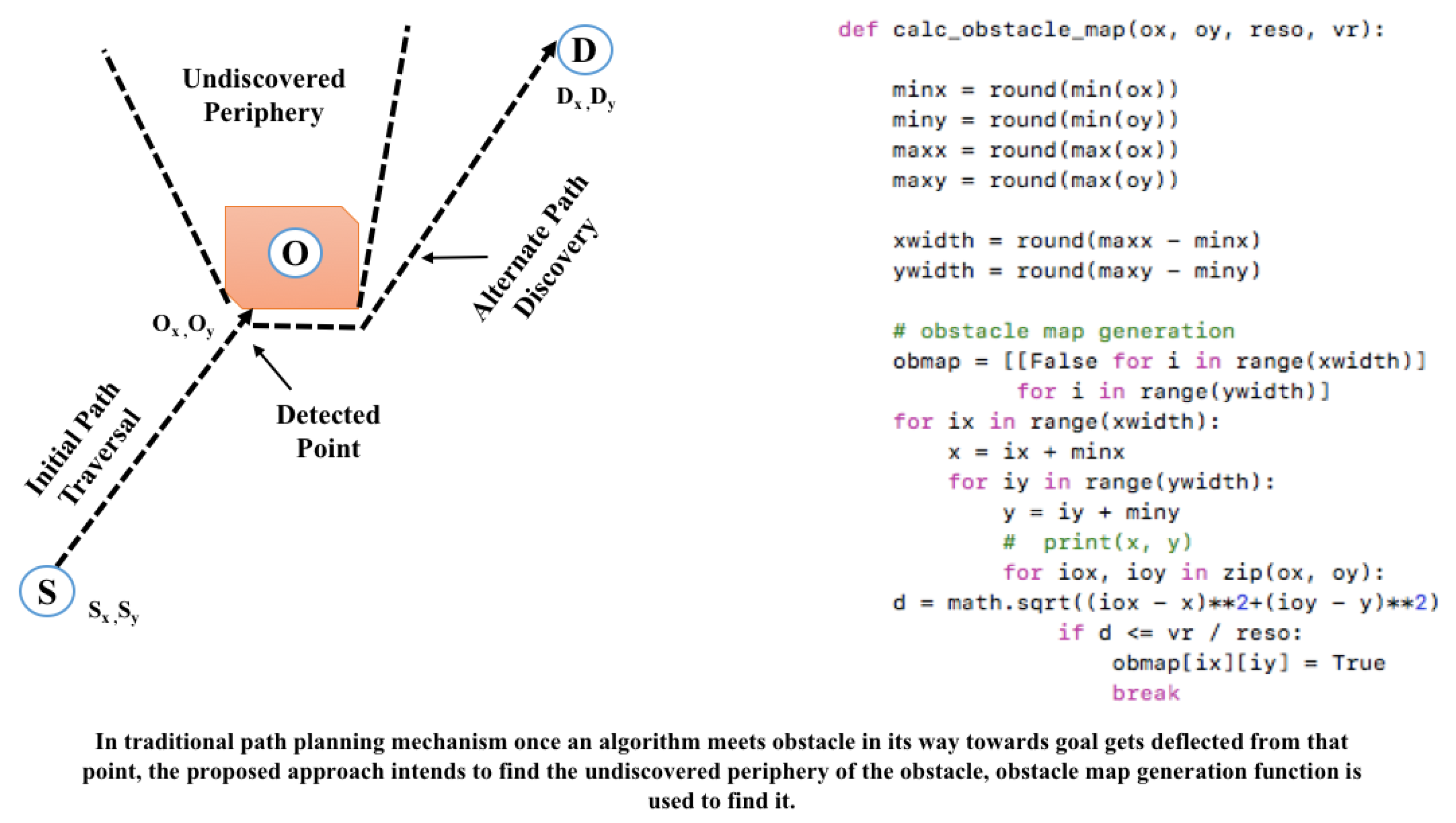
The entire hypothesis of path planning usually relies on the nature of obstacles. In a way, they are tracked and traced by any path planning algorithm which generally differentiates them from other techniques. Typically, the technique used for finding the optimal path starts probing from the source coordinates and keeps on navigating smoothly until it encounters any hindrance in the path. Usual practice narrates that once an algorithm is trapped in such circumstances, it searches for free space. Meantime it keeps on searching and moving to its adjacent point in search of free space. In actuality, it moves around the periphery of the obstacles. Thus, any technique that searches and finds the optimal path largely left over its time to get rid of this situation. Thus, if the circumference of an obstacle is large, then it will consume more time to travel from the obstacle’s periphery to the free space. In addition, the algorithm traverses one particular side of the obstacle from where it can find the free space, the rest part or region covered by the obstacle is left out, as at that moment it is of no use. Figure 1 depicts the scenario that mentions the undiscovered periphery of the obstacle that is not being traversed. This can degrade the efficiency of the system when there is more than one robot in any case and is stuck with the same obstacle Keeping this problem at the center, this paper proposes the use of the Snake Algorithm [20] with path planning algorithms  [21,22,23] to carry out our experiment. Figure 1 consists of the obstacle map generation method along with a pictorial representation of the problem. Here, in this paper, the snake algorithm is used with four different path planning algorithms in three different environments; the result obtained with the snake algorithm is then compared with the conventional path planning algorithm (without the snake algorithm), and the result is analyzed and compared in the result section, the working principles of all the algorithms used in this paper are described in the following sections.

5. Proposed Path Planning Method

This paper proposes the approach of using the snake algorithm for obstacle detection with path planning algorithms for robots to obtain better results. It is being achieved by implementing the snake algorithm to the map before applying path planning algorithms. The explanation of the proposed work is depicted in Figure 2, which shows the technical specification of the workspace along with the steps taken into account to carry out the experiment. The details of all the algorithms considered are described under the following subsection.

5.1. Snake Algorithm

According to Snake Algorithm discussed in Algorithm 1, Active contours represent the object boundary [24]. A snake is known as an active contour, which expands with the obstacles present in the image. It localizes itself in the image. A snake is a parametric curve that tries to move into a position where its energy is minimized. It is guided by various forces like image force and force incident from the outside factors, with the help of these forces, it recognizes the lines and edges present in the image. The goal is to find a contour that best approximates the perimeter or object outline of an object from a possibly noisy 2D image. These active contours are the obstacle while going for path planning for robots, whose boundary needs to be detected and identified. Snake algorithm first initializes the contour points in the configuration space and then it starts contracting to frame loop [25]. This loop signifies the presence of an obstacle. As it is a closed loop, it determines the complete periphery of the obstacle present. The behavior of the snake is caused by an external energy term that, in this case, determines that the snake feels attracted toward object boundaries. An energy function E is associated with the snake algorithm, which helps in finding the obstacle’s boundary in the configuration space. By applying the snake algorithm in configuration space, it will help in detecting the obstacle. Giving these details to the path planning algorithm will help in reducing the traverse space for finding a path. Thus, it helps the path planning algorithm to avoid traversing the space occupied by the obstacle. The concept of active contour was originally given by Kass et al for calculating snake energy is represented in the following Equations (3)–(5) [26,27].

$$E_{snake}^{*}\left(r\right)={\int }_0^1{E}_{snake}\left(v\left(s\right)\right)ds$$

(3)

$$E_{snake}^{*}\left(r\right)={\int }_0^1{E}_{int}\left(v\left(s\right)\right)+E_{snake}\left(v\left(s\right)\right)ds$$

(4)

$$E_{snake}^{*}\left(r\right)={\int }_0^1{E}_{int}\left(v\left(s\right)\right)+E_{img}\left(v\left(s\right)\right)+E_{con}\left(v\left(s\right)\right)ds$$

(5)

$$\begin{array}{c}\hfill E_{snake}^{*}\left(r\right)={\int }_0^1{E}_{int}\left(r\left(s\right)\right)ds+{\int }_0^1{E}_{img}\left(r\left(s\right)\right)ds\\ \hfill +{\int }_0^1{E}_{res}\left(r\left(s\right)\right)ds\end{array}$$

(6)

where $E_{int}$ represents the internal energy of the snake; $E_{img}$ is the image force; $E_{res}$ represents the external restraining force.

Parameters of the snake algorithm which play an essential role in the working of the snake Algorithm are Active Contours, Spatial Conflicts, and Displacement Operator and its working Principle rely on the factors like Internal Energy, External Energy, and Constraint Energy. Continuity and the smoothness of the obstacle comprise the internal energy of the snake Algorithm. Constraint Energy is the conditions put by the user to keep the snake algorithm away from certain specific features. It can be in the initial phase as well as in between the images. Aggregation of energies are called Constraint energy. The internal energy of the snake is written as Equation (7).

$$E_{int}^{*}=1/2(\alpha \left(s\right)\Vert v_s{\left(s\right)\Vert }^2+\beta \left(s\right)\Vert v_{ss}\left(s\right){\Vert }^2)$$

(7)

where the first-order term $\Vert v_s{\left(s\right)\Vert }^2$ gives the measure of the elasticity, while the second-order term $\Vert v_{ss}{\left(s\right)\Vert }^2$ gives a measure of the curvature. Snake Energy is being controlled by two coefficients $\alpha \left(s\right)$ and $\beta \left(s\right)$. Minimizing the values of these two parameters makes the snake more elastic and less rigid. The image forces $E_{img}$ to attract the snake to the desired feature in the reference maps. The external forces $E_{con}$ are attributed to some form of high-level map understanding. This helps snakes to unnecessarily get into the local minima. Another important aspect that is very much important while applying the snake algorithm is the minimization of energy of snake function. Now looking closer to the snake energy function in Equation (8). In addition, as per the fundamental lemma of the calculus of the variations, the functional derivates must vanish in the end leaving the equation should hold only for some arbitrary choice of ${\delta }_x\left(s\right)$.

$$\begin{array}{c}\hfill E_{int}^{*}=1/2(\alpha \left(s\right)\Vert v_s{\left(s\right)\Vert }^2+\beta \left(s\right)\Vert v_{ss}\left(s\right){\Vert }^2)\\ \hfill +E_{(}img)\left(v\left(s\right)\right)ds\end{array}$$

(8)

The following two equations, known as the Euler–Lagrange equations, give the minimized energy function. The minimum of the snake energy functional can now be found by solving these two independent Euler–Lagrange equations Equations (9) and (10).

$$\frac{d}{ds}\left({\alpha }_s\frac{d\widehat{x}\left(s\right)}{ds}\right)+\frac{d^2}{d{s}^2}\left({\beta }_s\frac{d^2\widehat{x}\left(s\right)}{d{s}^2}\right)+\frac{\delta E_{(}img)}{\delta x}{\mid }_{\widehat{x},\widehat{y}}=0$$

(9)

$$\frac{d}{ds}\left({\alpha }_s\frac{d\widehat{y}\left(s\right)}{ds}\right)+\frac{d^2}{d{s}^2}\left({\beta }_s\frac{d^2\widehat{y}\left(s\right)}{d{s}^2}\right)+\frac{\delta E_{(}img)}{\delta y}{\mid }_{\widehat{x},\widehat{y}}=0$$

(10)

Algorithm 1 Snake Algorithm to detect contour.

$Computationoffunctionv/ssnakes(I,v)$ $E\_image=ComputeImageEnergy\left(I\right);$ while$not$$generated$do    $F\_cont=alpha.weight\ast Derivative\_contour(v,2);$    $F\_curv=beta.weight\ast Derivative\_contour(v,4);$    $F\_image=interprate2(Eimage,v(:,2\left)v\right(:,1\left)\right)$    $F\_image\_norm=k\ast F\_image./norm(F\_image).weight.;$    $F\_con=input\_Forces\left(\right);$    $F\_internal=F\_cont+external.weight\ast Fcurv;$    $F\_external=external.weight\ast (F\_external,F\_internal);$    $v=updateSnake(v,F\_external,F\_internal);$    $checkConverge\left(\right);$    $end$ end while $functionEimage=generateImageEnergy\left(I\right)$ $[C,C_x,C_y,C_{x}x,C_{y}y]=generateGradients\left(I\right);$ $E\_line=I;$ $E\_edge=\left[{(C_x{.}^2+C_y{.}^2)}^{.}5\right];$ $E\_term=((C_x^2.2\ast C_{y}y\ast C_{x}y.C_x\ast C_y+C_{x}x.C_y^2)/{(1+C_x^2+C_x^2)}^{(}1.5))$ $E\_image=weight.line\ast Eline+weight.edge\ast Eedge+weight.term\ast Eterm;$ $end$

Some advantages of the snake algorithm are like: Time Optimisation is appreciable as the other technique gets the free space separated from the overall space. Boundary Coordinate information will be present with the robot; thus, repeated calculation overhead will be minimized. The multi-robot system can be implemented efficiently due to overall less computation time. Furthermore, the disadvantages of the snake algorithm while applying for path planning are that it depends on the number of spacing and control points, and it is not trivial to prevent self-curve intersection.

5.2. Path Planning Method

This paper proposes a hybrid way to optimize the problem of robot path planning. To do so here, we propose the concept of snake algorithm along with the traditional path planning algorithm [28]. As discussed in the previous section, the working of the snake function helps in finding the contours present in the workspace which reduces the effort applied by the path planning algorithms to reach the robot from its source position to the destination [29,30]. Here in this paper, we have considered three different path planning algorithms along with the snake algorithm to find the solution. We have considered three algorithms namely A*, PRM, RRT & RRT Smooth [31]. The reason to pick this algorithm among all the available algorithms for path planning is that these three algorithms differ from each other entire in terms of their working mechanism. The working mechanism here refers to the working of algorithms while finding the best route for the robot, or it can also be defined as the traversing behavior of these three algorithms that are entirely different from each other. The purpose of picking algorithms whose traversing behavior should differ is that when it is combined with the snake algorithm, it will validate the concept in multiple aspects. The working [32,33] of A* is based on the concept of selecting the next best node based on the heuristic function [34], whereas PRM is quite fast as compared to A*. The working of PRM mainly focuses [35] on selecting the random nodes out of available ones in the workspace, whereas the working of RRT is based on creating a parent-child node tree and it keeps on creating the tree till it reaches the destination. We also have considered the advanced version of RRT [36] in this paper. Finally, we have combined all these algorithms to form a hybrid combination with the snake algorithm to test the proposed hypothesis. Finally, the result obtained was very encouraging and is presented in the later section of the manuscript [37].

5.3. Work Flowgraph of Proposed Work

In the above section, the working principles of the Algorithm (A*, PRM, RRT, and RRT-S) are discussed in detail, and the working procedure is summarised in the form of the flow graph in Figure 3. The graph explains the basic steps of the algorithms, initially the presence of contour is detected by the snake algorithm (Here in this case contours are the obstacles present in the reference maps) and then the nodes are initialized, and the complete periphery of an obstacle is then traced out which is being provided to the path planning algorithms, and then points the unique procedures followed by each algorithm is carried out. In the end output of each procedure would be the parameter taken to test the results shown in

Table 2. Comparative analysis of results obtained on the reference maps using path planning algorithms with snake algorithms and without snake algorithms.

		With Snake Algorithm			Without Snake Algorithm
Reference Map	Path Planning Algorithms	Path Length	Time Taken	No. of Moves	Path Length	Time Taken	No. of Moves
Maze	A*	351	143	19	352	157	21
	PRM	371	12	24	374	13	29
	RRT	451	227	440	455	249	484
	RRTS	442	178	436	445	195	479
R.O	A*	285	89	12	290	97	13
	PRM	294	20	21	298	23	23
	RRT	340	74	327	348	81	359
	RRTS	350	90	339	357	98	373
Dense	A*	127	116	06	129	128	07
	PRM	127	41	14	128	49	15
	RRT	160	15	155	166	18	170
	RRTS	145	12	142	149	15	156

.

6. Results and Discussion

The results obtained as per the proposed work are explained in this section. There are a total of 12 results recorded and demonstrated in the paper. It is divided into three different cases, and each case has four different results; certain assumptions have been made, which remain constant for all results. like $robotsize=1.0$ and $gridsize=1.0$. To measure the path length we have assumed 1 cm = 38 px. The following table also illustrates some conditions taken for experimentation. $s_x$ and $s_y$ are the values of source coordinates while $g_x$ and $g_y$ are the values of goal coordinates.

In all three different cases, the first step is to take the appropriate map as input. After choosing the proper map as input, the next step is to implement the snake algorithm over it, the function of the snake algorithm is to trace the obstacle present in it. The space occupied by these obstacles in the map is identified by the snake algorithm; these particular spaces are recognized as the complex space or the space occupied by the obstacle. The result of the snake algorithms using the variables; $O_x, O_y, reso, vr$, which is then given as input to the path planning algorithms.

After receiving the output from the previous step, i.e., implementation of the snake algorithm, the next step is to implement the path planning algorithms for finding optimal paths. Here the path planning algorithms need to traverse only free space out of the total workspace, which is a usual practice in any path planning problem. The pre-run of snake algorithms on the map has the complete coordinate details of obstacles present on the map, it provides these details to the next stage which is running the path planning algorithms, the advantage of the first step is that it selectively provides the free space for path findings, with the help of which the actual map which is to be traversed by the path planning algorithms is reduced; thus, the complex space or the obstacle occupied space can be skipped by the path planning algorithms. The red line in the map of the last stage of each case represents the path obtained by the respective algorithms. The overall result is presented in three cases.

Case.1,: Maze image is taken as input for implementing the snake algorithm over it. In the next stage, it experiments with A*, PRM, RRT, and RRT-S. The result obtained after implementing all four path planning algorithms with the snake algorithm is presented in Figure 4, Case.1. In this case, it is being observed that path length is minimum with A* algorithm, while the time taken is less with PRM and No. of Moves is least with the PRM. In Case.2, the Random Obstacle image is taken as input; the rest of the two-step remain the same as in case 1. The result obtained after this is presented in Figure 4, Case 2. The results show that the path length is almost the same with a slight difference between A* and PRM, time taken is less with PRM and No. of Moves is least with the A*. In Case.3, the Dense image (Image of NIT Raipur campus) is taken as input, and after repeating the two steps stated above for case 1 and case 2. The result obtained is presented in Figure 4, Case 3. In this case, it is observed that the path length is minimum with A* and PRM algorithm, while the time taken is less with RRT and RRT-S and No. of Moves is least with the A*.

Table 1 presents the comparison of results of each algorithm in all three scenarios and the Figure 5, Figure 6 and Figure 7 shows the outcome of the proposed work and compares it with the conventional work (algorithms without snake), i.e., the association of path planning algorithms with snake algorithms, Figure 5 shows the path length comparison and it is evident from the graphs that there is a minor difference in the path length. Figure 6 shows the comparison of time taken by the algorithm and it depicts that the time taken is less when using the path planning algorithm with the snake algorithm. Figure 7 shows the comparison of No. of moves taken by the algorithm and it is also showing the very minimal difference. The main advantage of using the snake algorithm is the reduced time taken by the algorithm which can be utilized in many applications based on multi-robot systems. The reason is that in a multi-robot system if all the robots are aware of the obstacle with its position, the summation of time gained by all the robots will make the system more efficient.

7. Conclusions

To conclude the idea proposed in this paper, it is required to mention that the proposed work is not merely an amendment of any existing work and comparison with other literature; indeed the effort is to distend the application and acceptability of path planning solutions to more areas. Though we presented a detailed analysis and comparison of output in the result section, the author would like to mention here the broad scope of this work. This paper tries to bring the concept of knowing the presence of obstacles in the workspace like its location, shape, and size by knowing its complete periphery. Getting this knowledge in advance will help in planning the path in a much better and optimized way. The paper also analyzed the comparison of results without using the snake algorithm, using the snake algorithm as a preliminary step to detect algorithms has some advantages over the conventional approach. Path length seems to remain the same while the time taken by the algorithm is representing an advantage gain of ten percent approximately while the number of moves also shows a one to two percent gain. The experiment was carried out on three different maps which have the potential to reveal each path planning algorithm’s capability, the same has been presented and compared in this paper. It can be employed for landing unnamed aerial vehicles, drones, and strategic planning in critical conditions. This method could also contribute to executing some crucial military missions with the help of robots. Though we have tested it with specific limitations, it can be implemented in some more diverse conditions with a few more techniques to observe the results. A dynamic environment or multi robots scenario can also gain the advantage of this work. The extension of this work could be to optimize the computation time in a multi-robot system.