Author Contributions
Conceptualization and Methodology: D.R., A.F.I. and F.S.; Software and validation: Z.H., A.A.Z., D.R., A.F.I.; Formal Analysis: Z.H., A.A.Z., D.R., F.S., H.H. and A.F.I.; Investigation: Z.H., A.A.Z., D.R., H.H. and A.F.I.; Data curation: Z.H., A.A.Z., D.R., F.S., H.H. and A.F.I.; Writing—original draft preparation: Z.H., A.A.Z. and A.F.I.; Writing—review and editing: Z.H., A.A.Z., D.R., F.S., H.H. and A.F.I.; Visualization: Z.H., A.A.Z., A.F.I. and H.H.; Supervision: A.F.I.; Project Administration: A.F.I. and D.R.; Funding acquisition: F.S. and A.F.I. All authors have read and agreed to the published version of the manuscript.
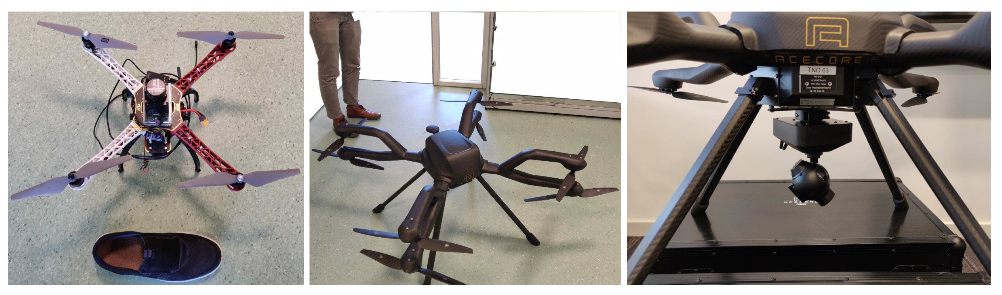
Figure 1.
Examples of the drones available in the Intelligent Autonomous Systems group at TNO: (
left) a small device for proof-of-concept testing; shoe for scale. (
Center) a heavy-duty AceCore NEO drone capable of carrying payloads in excess of 8kg outside and in normal weather conditions. (
Right) a bottom-mounted gimbal for visual data collection, possibly to be analyzed onboard for fast victim recognition. The presented work in this article has not been deployed under real-world conditions, but TNO and VTT are planning to conduct real-world tests in the near future; cf. [
9,
24].
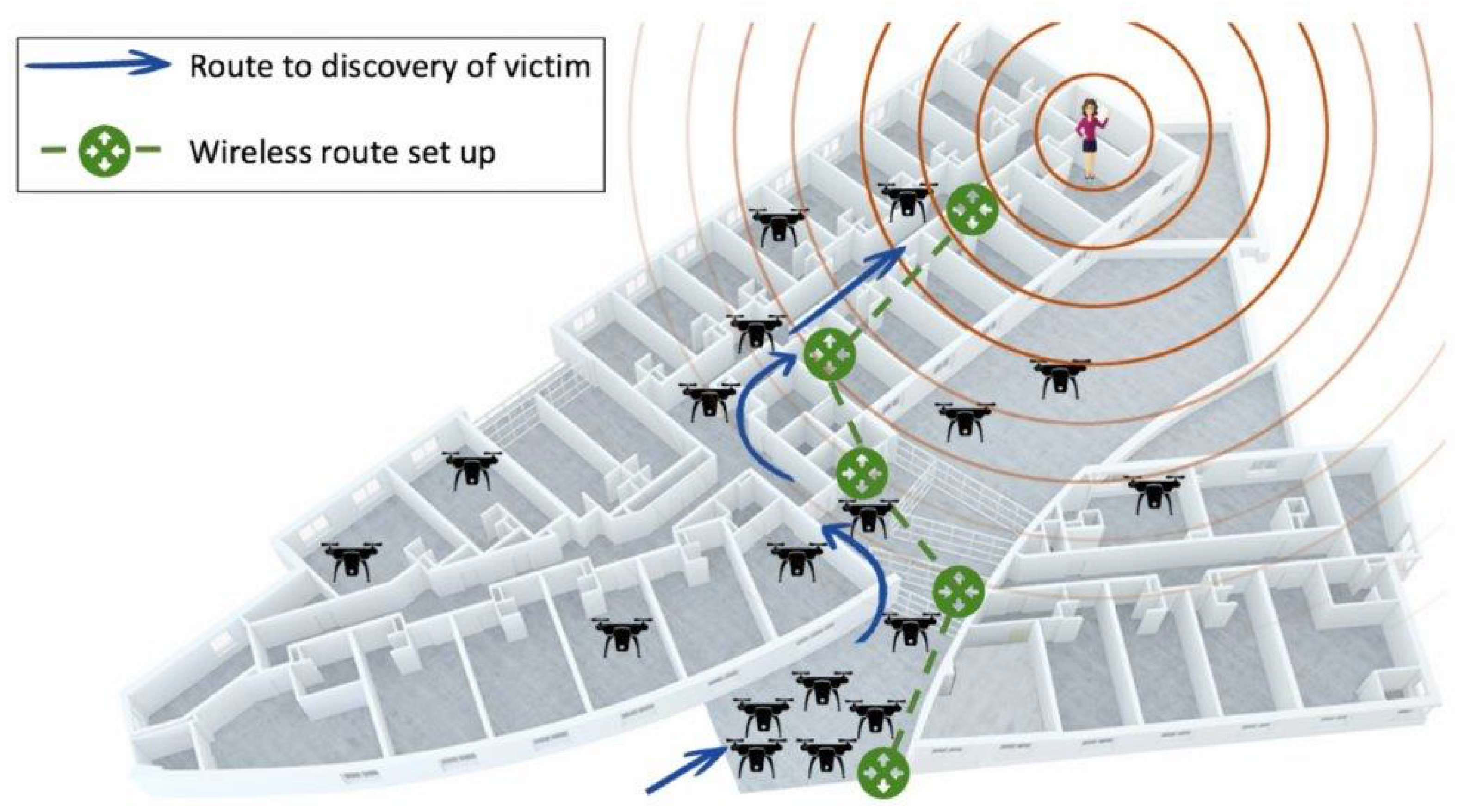
Figure 2.
An indoor Search and Rescue (SAR) scenario where the victim sends out a distress signal to guide a search conducted by autonomous robotic agents. On discovery of the victim, the agents create an optimal relay link (by optimizing various aspects such as time, cost, length of the link, etc.) to connect the victim to the base station. The other scattered agents not involved in the relay can be called back to the base.
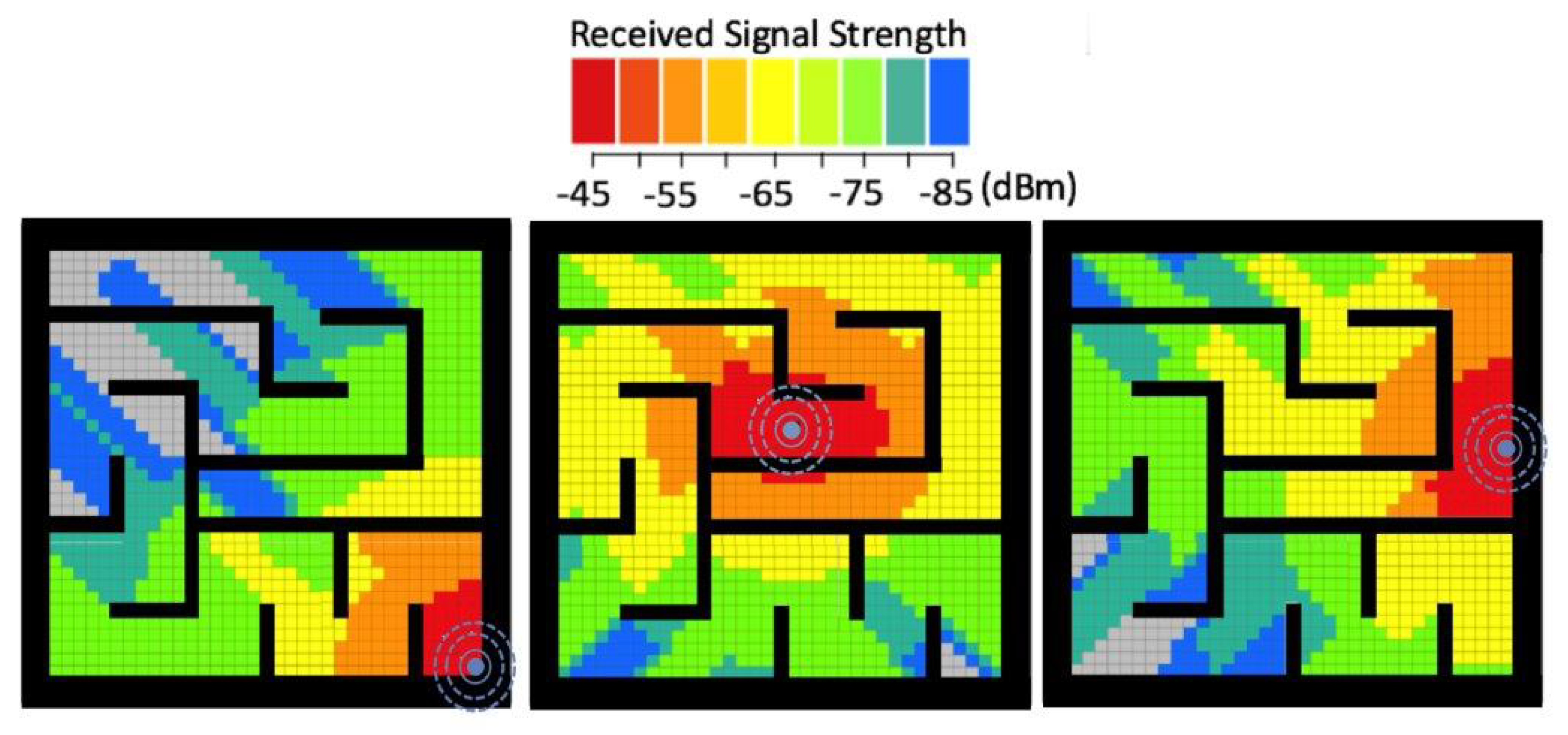
Figure 3.
Color-coded illustration of the beacon signal power received across the maze. The signal attenuates with distance and across the obstacles (walls), shown here in black color. The attenuation is a function of the distance. The signal undergoes added attenuation across walls due to shadowing.
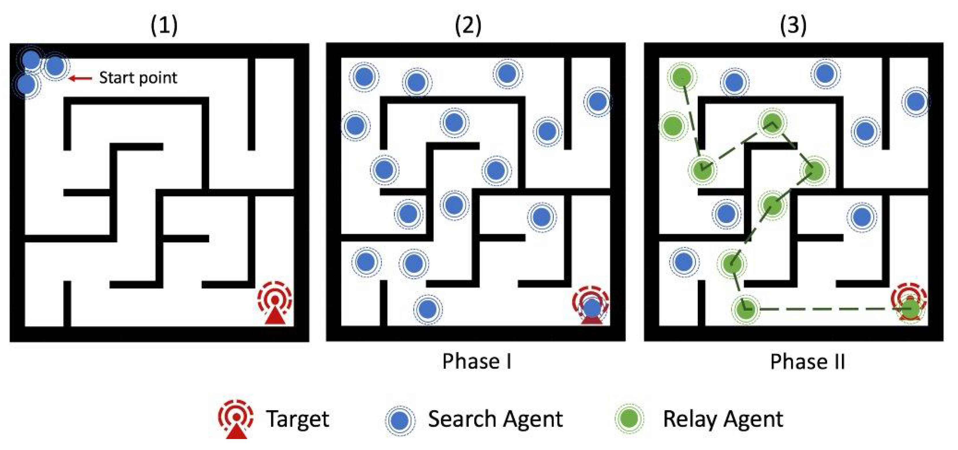
Figure 4.
The indoor search is translated into a maze-solving problem. Just as with the indoor search introduced in
Figure 2, the agents enter the maze at a specific start location / point (1), traverse the maze in search of the target (depicting the victim) in Phase I, shown in (2), and then (in Phase II) calculate the shortest and cheapest route amongst the scattered agents (3) to form a relay network.
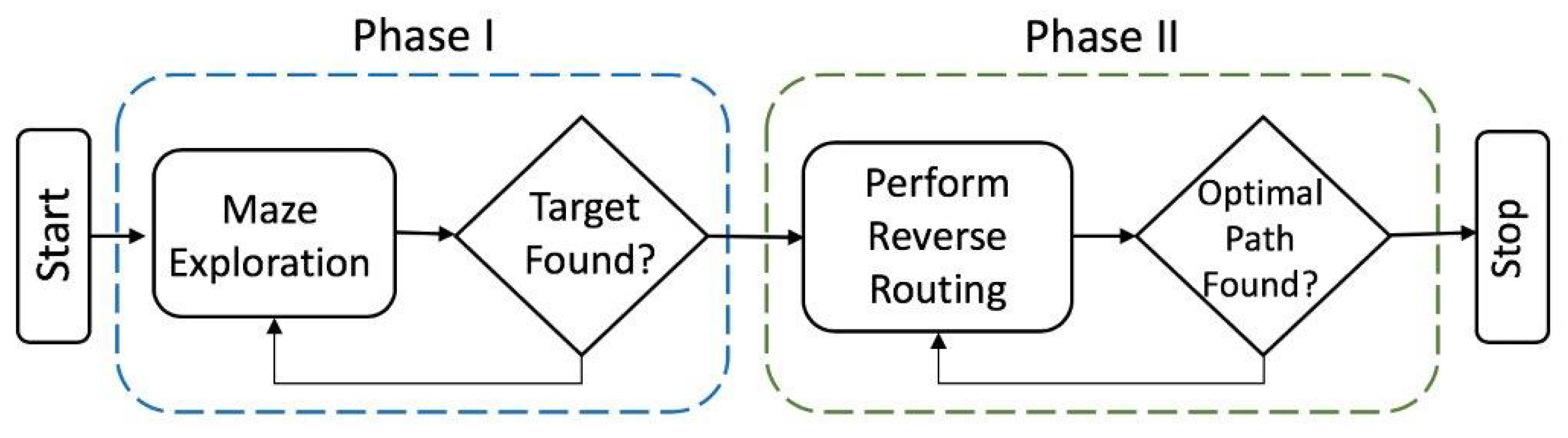
Figure 5.
The search and rescue process can be seen as two sequential phases: Phase I, where the search is conducted in an environment; and Phase II, where the extraction of an item or person from the environment is realized (i.e., the rescue part). For details, see
Section 3.2.
Figure 5.
The search and rescue process can be seen as two sequential phases: Phase I, where the search is conducted in an environment; and Phase II, where the extraction of an item or person from the environment is realized (i.e., the rescue part). For details, see
Section 3.2.
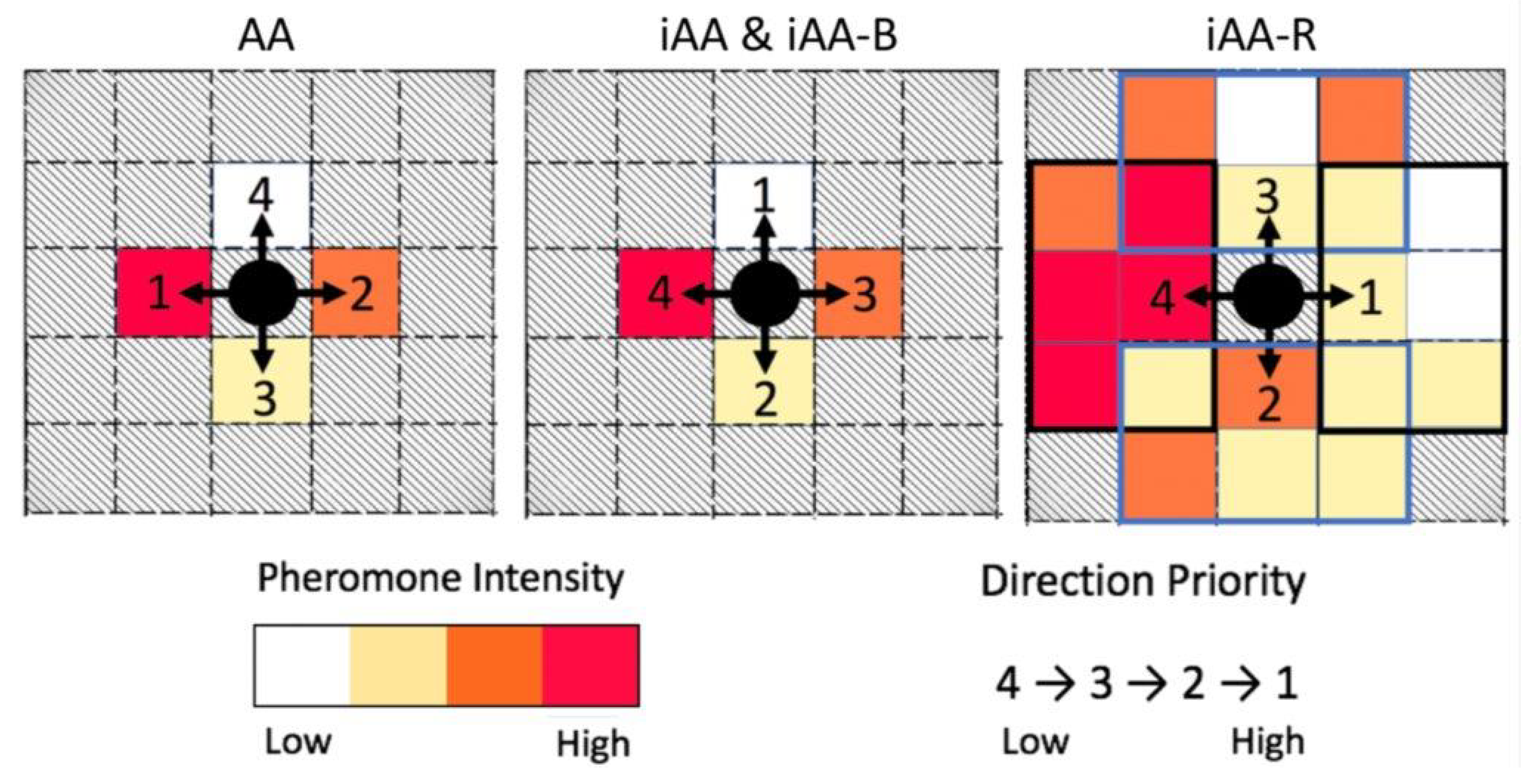
Figure 6.
All AA-based decision-making models prioritize their 5 possible directions of movement (1–4 are shown above, with the option to remain stationary being the 5th). AA prioritizes moving to a cell with a higher pheromone level, while all iAA-based models prefer moving to a cell with a lower pheromone concentration. The iAA-R algorithm (rightmost image, above) checks for average pheromone in neighboring regions, while the other three approaches (AA, iAA, and iAA-B) only check pheromone levels in the immediate neighboring cells.
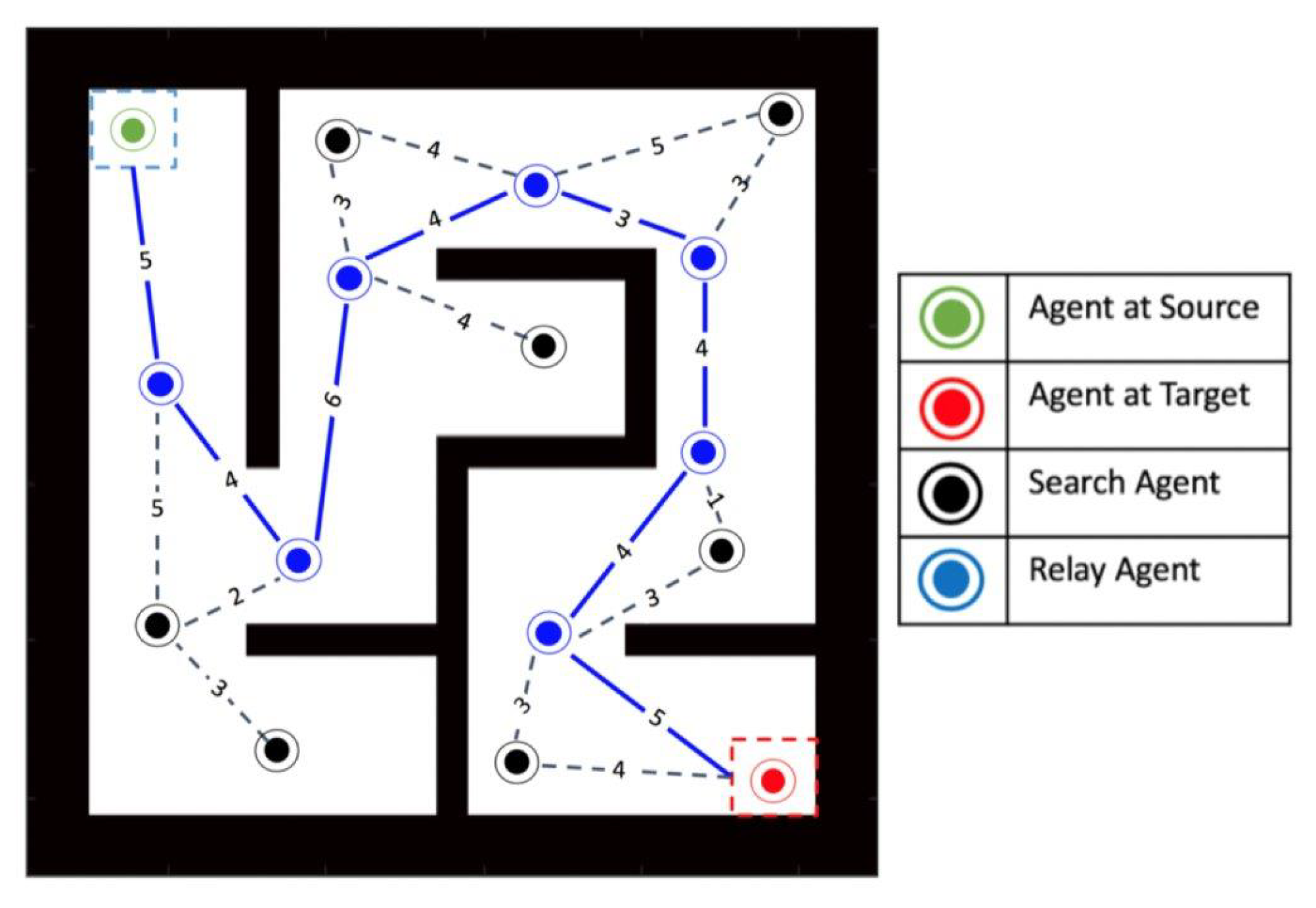
Figure 7.
The path cost calculations, having found an optimal path back to the source. At each hop, the algorithm favors the link with the lowest cost associated with it (indicated by the integers).
Figure 7.
The path cost calculations, having found an optimal path back to the source. At each hop, the algorithm favors the link with the lowest cost associated with it (indicated by the integers).
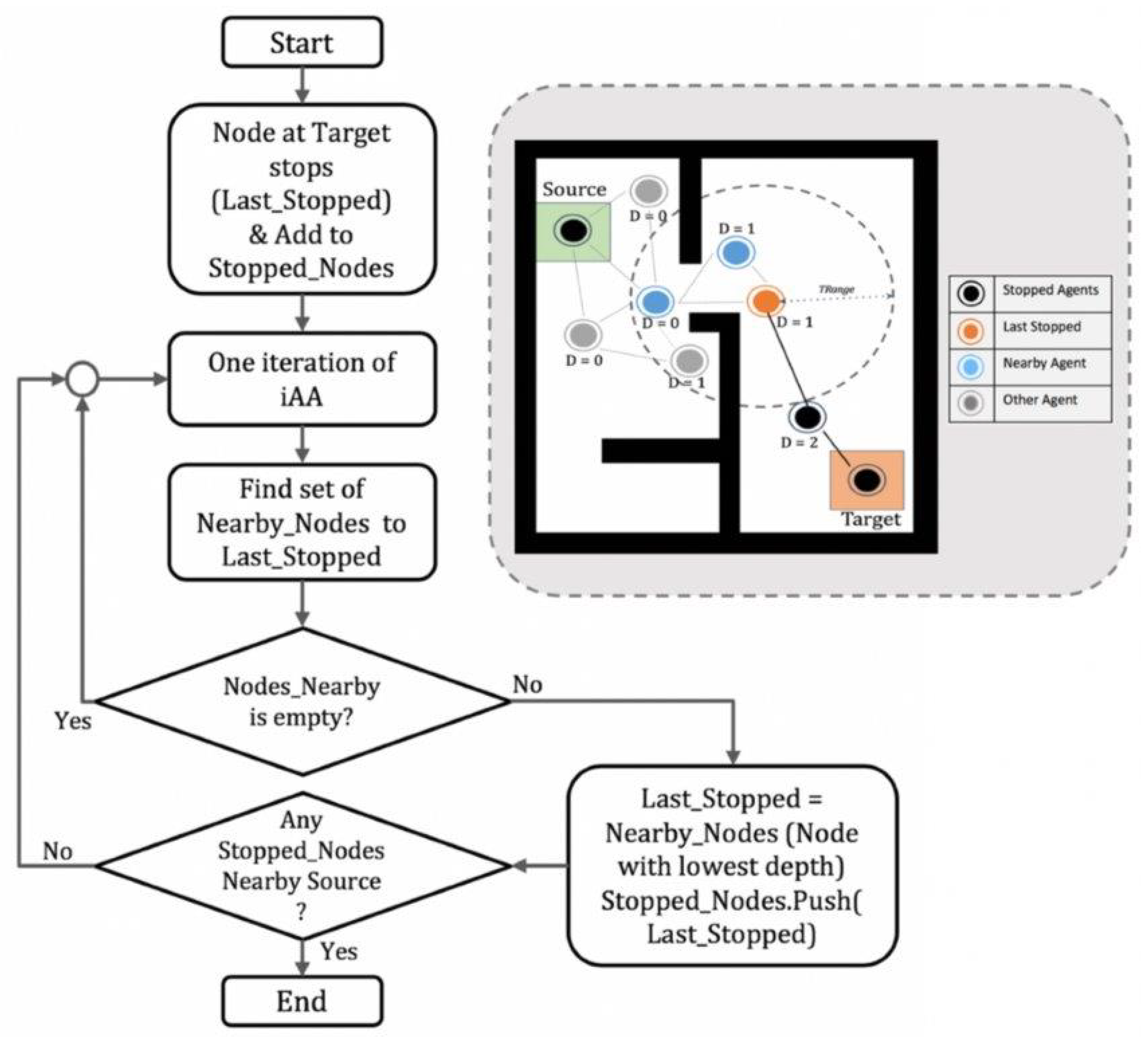
Figure 8.
Flowchart describing the working of the system in phase II. The last stopped node considers only the nodes within its communication range as its neighbors in the calculations. If there are no nodes within its communication range, the iAA simulation is restarted to move the nodes until at least one neighbor appears.
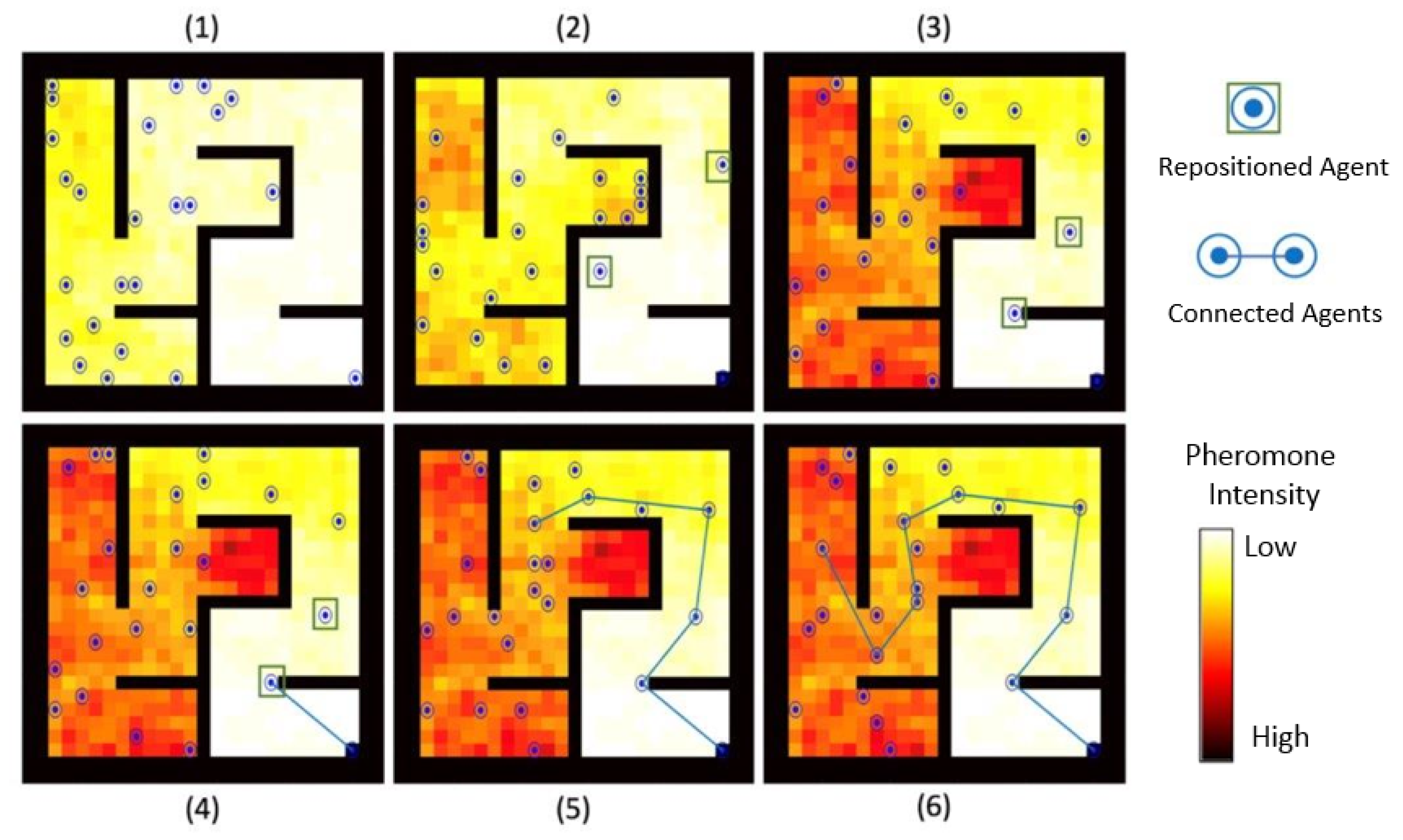
Figure 9.
A visual example showing the proposed approach: in (1) the target is located and the agent stops and starts looking for nearby agents, which (2) continue exploring. In (3) one agent is nearby, in (4) a link to that agent is created, and it stops. This process continues (5) to other agents, using the least depth as the guiding factor until (6) the process ends when the reached agent is near the source, causing the Dijkstra algorithm to terminate.
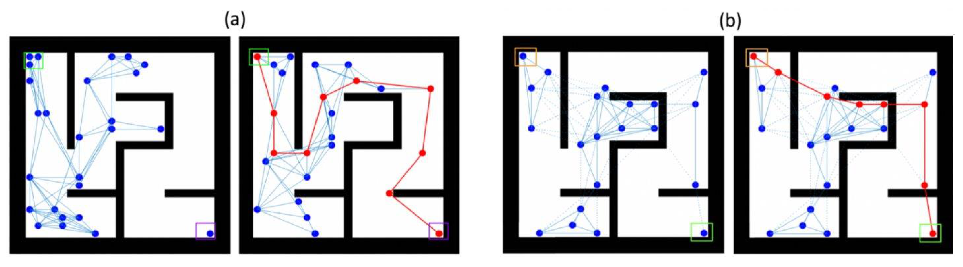
Figure 10.
Reverse route set up using the modified Dijkstra approach with implementation of both (a) impenetrable and (b) penetrable walls. The path length in the case of penetrable walls is much shorter than the former. However, this is heavily dependent on the material of the walls in the search space, which shows it could have a heavy influence on the performance of our technique.
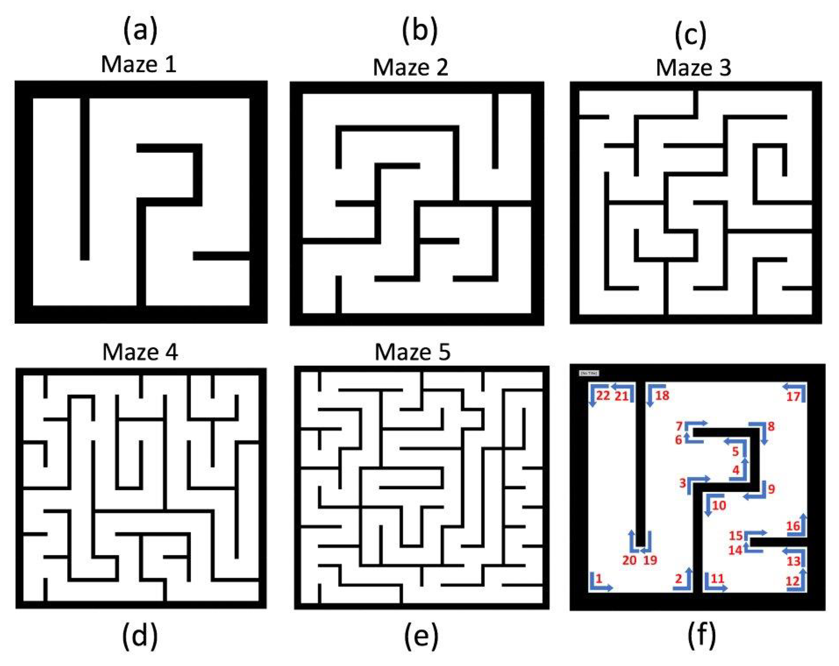
Figure 11.
(
a–
e) show the complexities of the 5 sample mazes (henceforth: M1-M5) referenced in this paper, cf.
Table 3 for a numerical comparison. These are provided as examples. In total, 10 different layouts were generated for each complexity listed in
Table 3 to further gauge the affect of randomness on the results. Maze (
b) was previously used in
Figure 4. The last panel, (
f), illustrates how we calculate maze complexity, using the example of maze (
a): the complexity is the number of 90 degree turns an agent can make in the maze, cf. (
f).
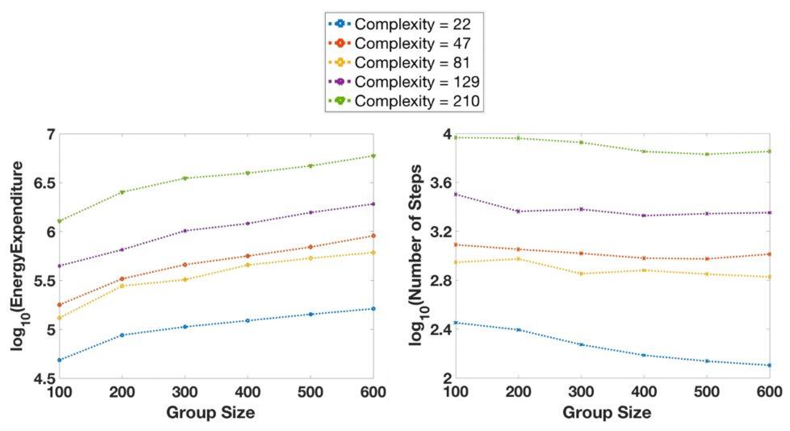
Figure 12.
Number of steps to solve the maze and the associated energy expenditure as a function of search group size used to solve the maze, for 5 different maze complexities. The graphs on the leftplot the energy expenditure while the graphs on the rightplot the number of steps.
Figure 12.
Number of steps to solve the maze and the associated energy expenditure as a function of search group size used to solve the maze, for 5 different maze complexities. The graphs on the leftplot the energy expenditure while the graphs on the rightplot the number of steps.
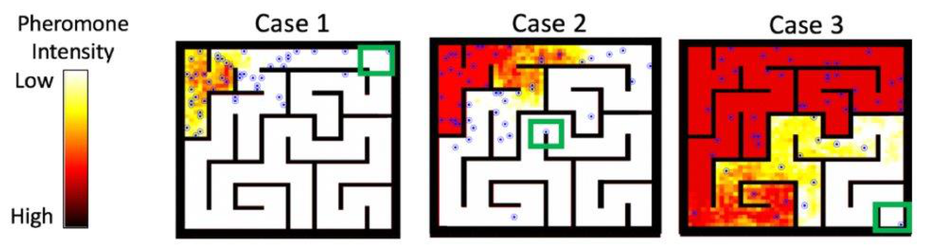
Figure 13.
Three possible locations of a victim inside a maze and the resulting final pheromone levels.
Figure 14 compares the resulting maze exploration and the number of steps taken to achieve it.
Figure 13.
Three possible locations of a victim inside a maze and the resulting final pheromone levels.
Figure 14 compares the resulting maze exploration and the number of steps taken to achieve it.
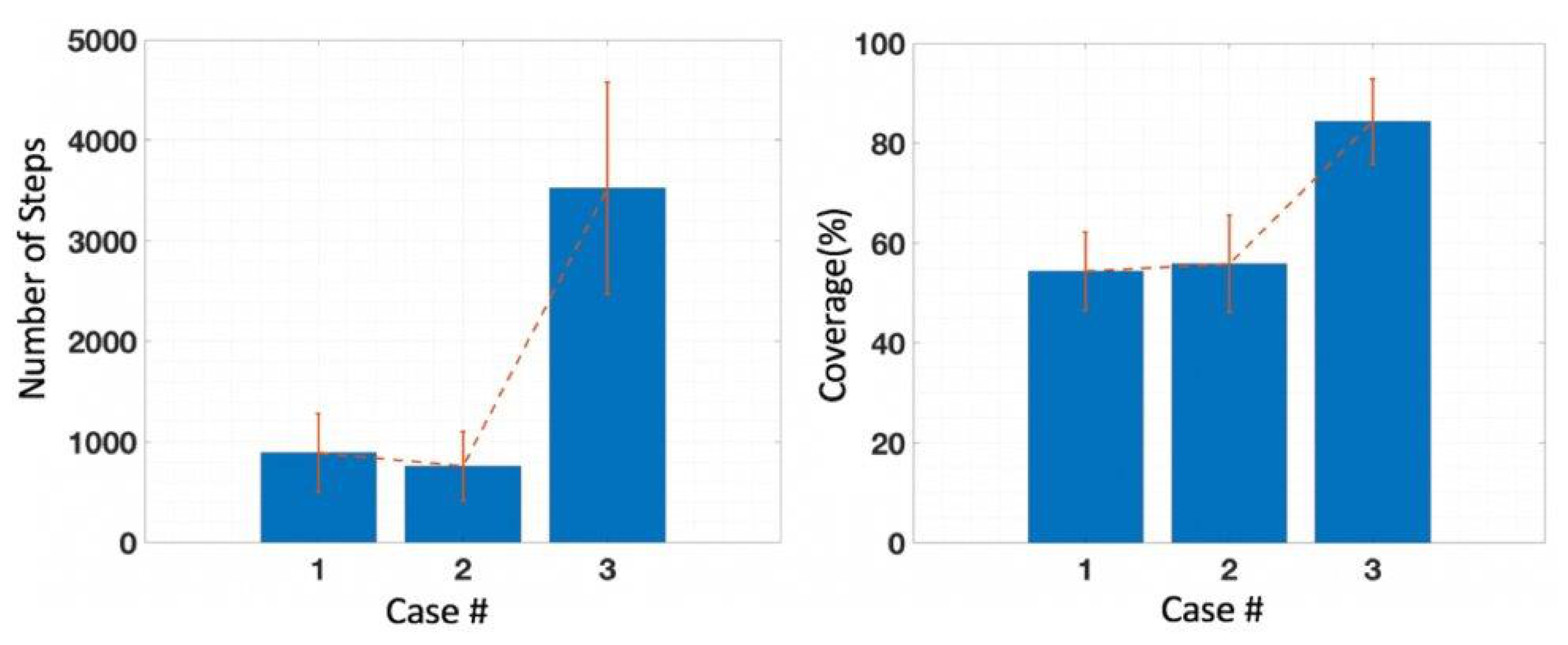
Figure 14.
The achieved maze coverage (
right), measured as the percentage of explored cells in the maze, and the corresponding number of steps (
left) for each of the three mazes shown in
Figure 13. Exploration is a by-product of the search process.
Figure 14.
The achieved maze coverage (
right), measured as the percentage of explored cells in the maze, and the corresponding number of steps (
left) for each of the three mazes shown in
Figure 13. Exploration is a by-product of the search process.
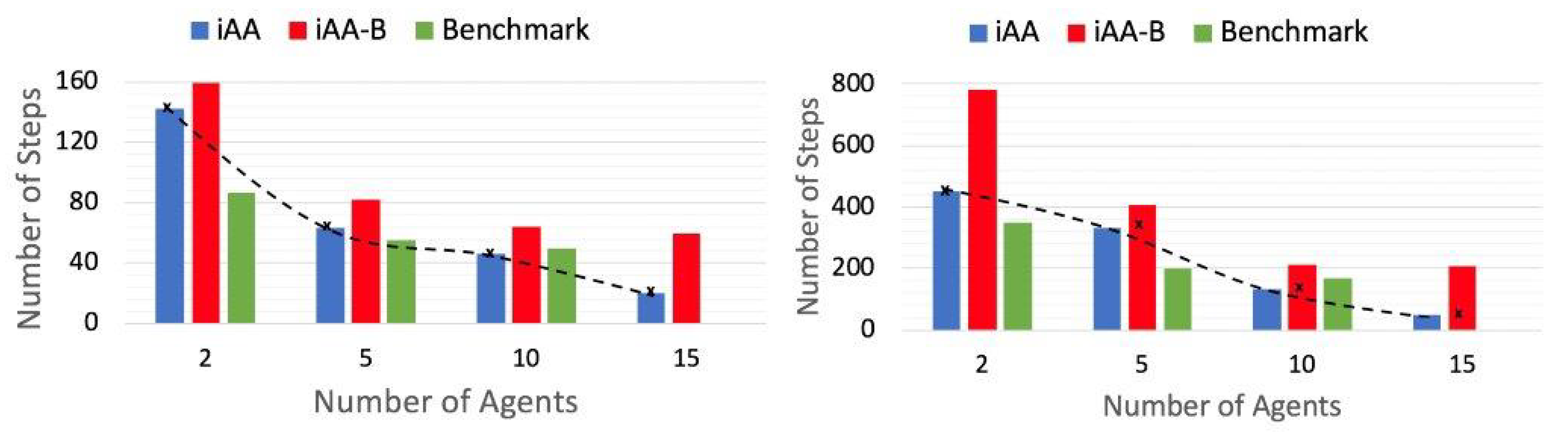
Figure 15.
While the benchmark outperforms our approaches (iAA and iAA-B) for small group sizes, our technique iAA beats the benchmark [
89] as the swarm size increases. Furthermore, an extended study shows that the trend of improvement in iAA is even more favorable as the swarm size continues to increase. This change in performance can be attributed to the swarming effect, which is better observed for a considerable search group size and does not show as much for a very small group (two agents or so).
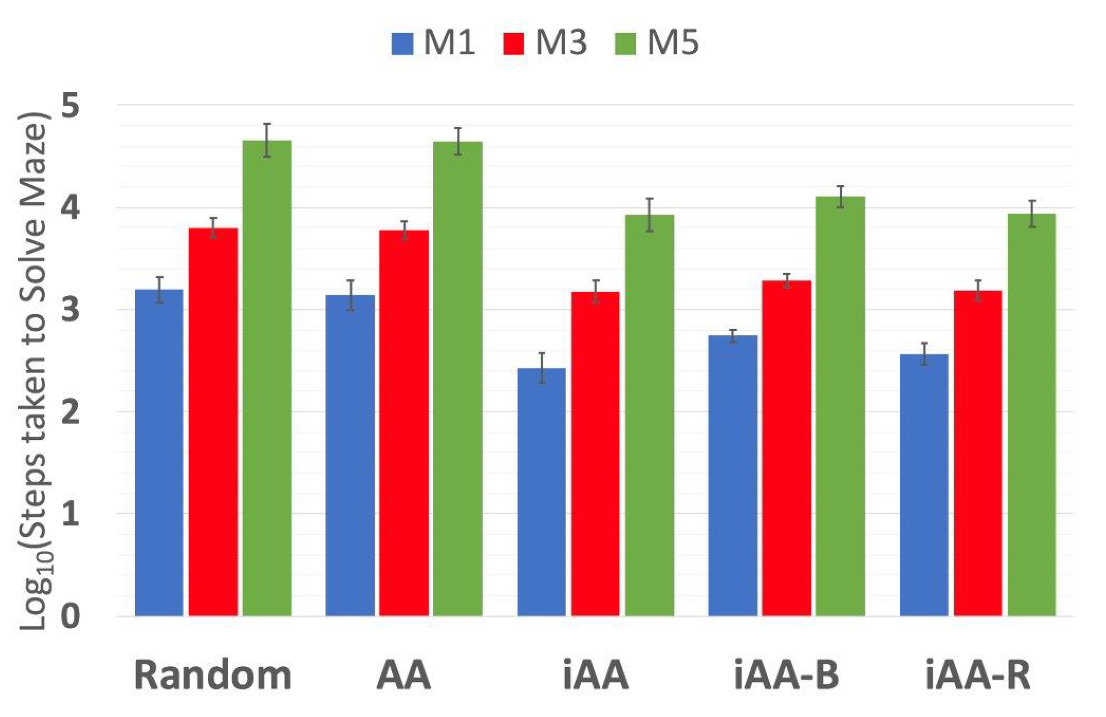
Figure 16.
Comparing the performance of the 4 AA-based models and a random movement solution in solving the 3 of the sample mazes (M1, M3 and M5), which are of different sizes and complexities, with 100 ants each.
Figure 16.
Comparing the performance of the 4 AA-based models and a random movement solution in solving the 3 of the sample mazes (M1, M3 and M5), which are of different sizes and complexities, with 100 ants each.
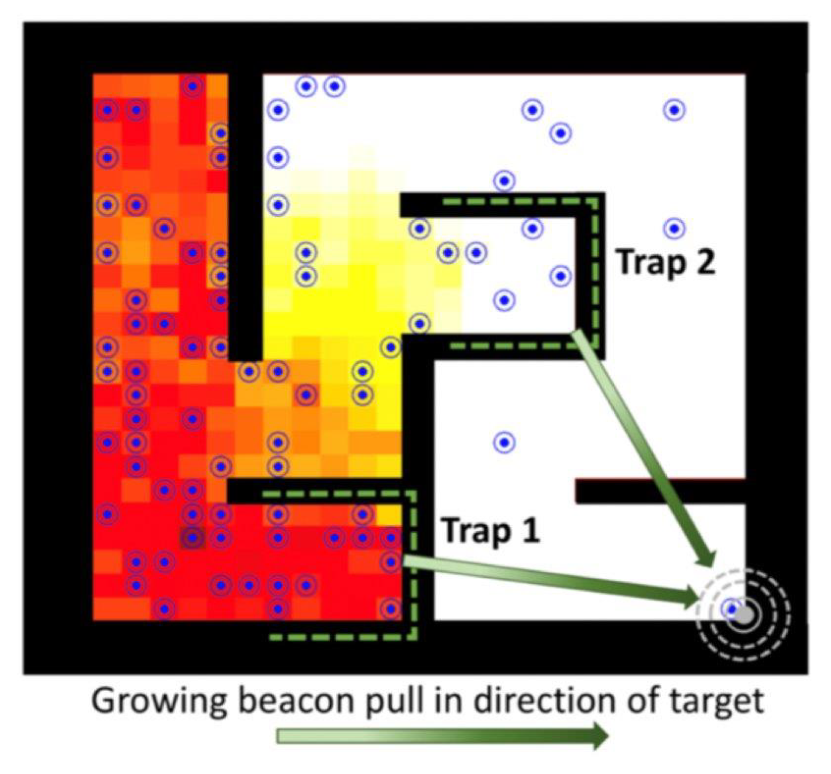
Figure 17.
Inverted AA with beacon initialization for pheromone intensities can lead agents into the traps, marked as green-dashed U-shaped walls in the figure, as they tend to blindly follow a positive pheromone gradient and are unable to go around these obstacles.
Figure 17.
Inverted AA with beacon initialization for pheromone intensities can lead agents into the traps, marked as green-dashed U-shaped walls in the figure, as they tend to blindly follow a positive pheromone gradient and are unable to go around these obstacles.
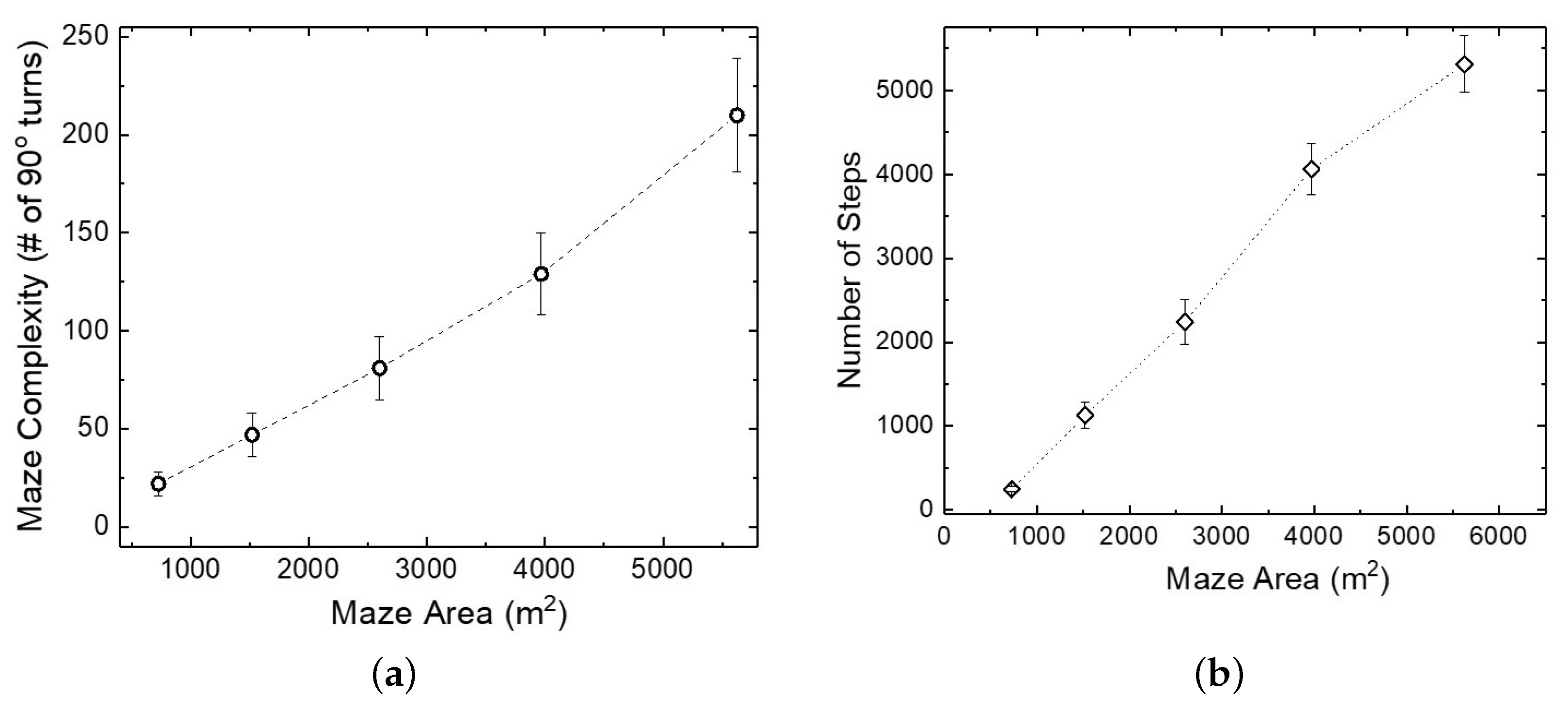
Figure 18.
Performance of iAA algorithm as a function of variable maze size and maze complexity (cf.
Table 3), with a constant search group of 100 agents. The plot in (
a) shows the (weakly supra-linear) growth in complexity while (
b) compares performance on the basis of the number of steps.
Figure 18.
Performance of iAA algorithm as a function of variable maze size and maze complexity (cf.
Table 3), with a constant search group of 100 agents. The plot in (
a) shows the (weakly supra-linear) growth in complexity while (
b) compares performance on the basis of the number of steps.
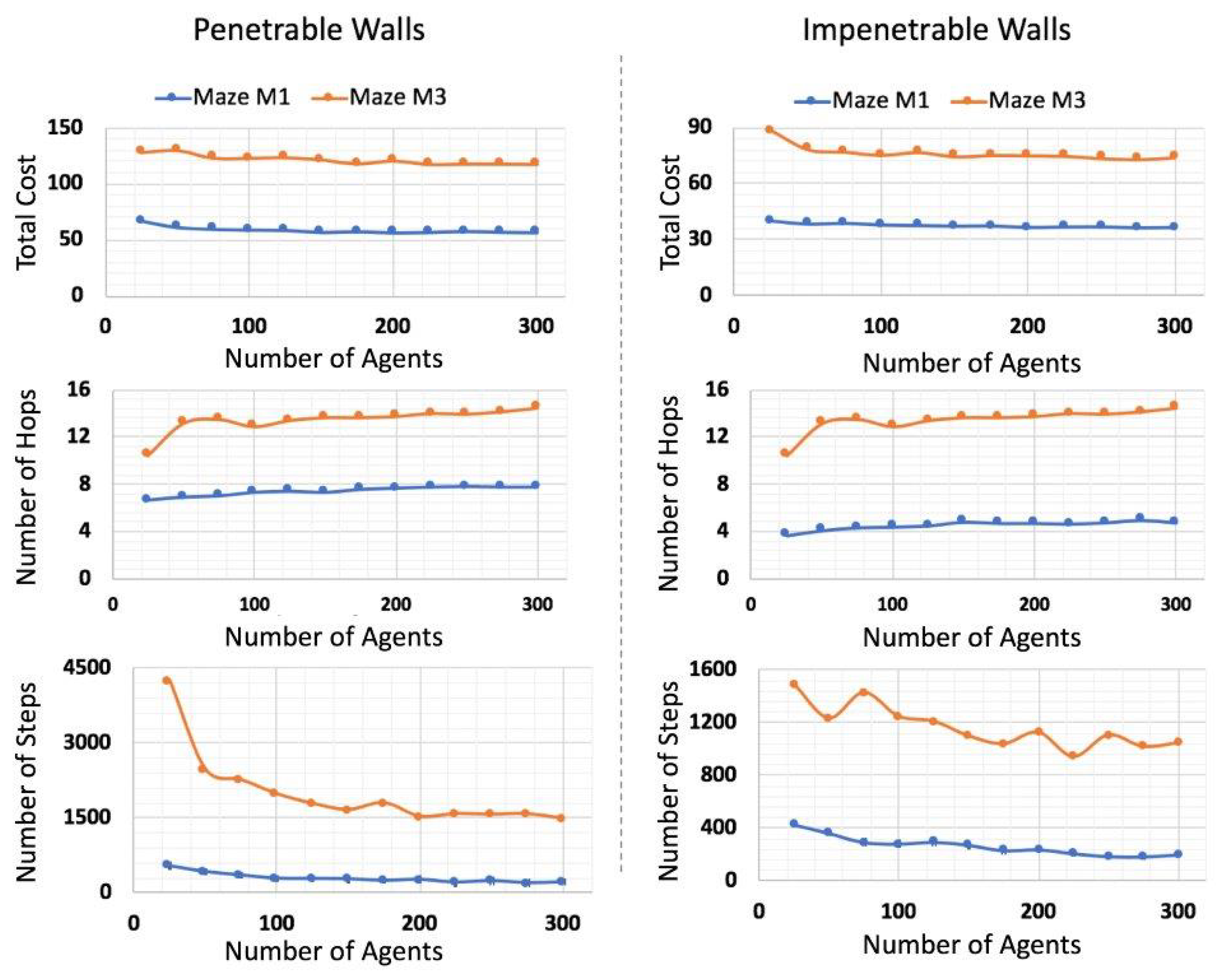
Figure 19.
Performance analysis of Phase II in terms of number of steps (or iterations of the algorithm) taken to solve the maze, number of hops in the final relay network formed and the total cost of the relay path found (measured in distance), as tested for 2 maze complexities, M1 and M3.
Figure 19.
Performance analysis of Phase II in terms of number of steps (or iterations of the algorithm) taken to solve the maze, number of hops in the final relay network formed and the total cost of the relay path found (measured in distance), as tested for 2 maze complexities, M1 and M3.
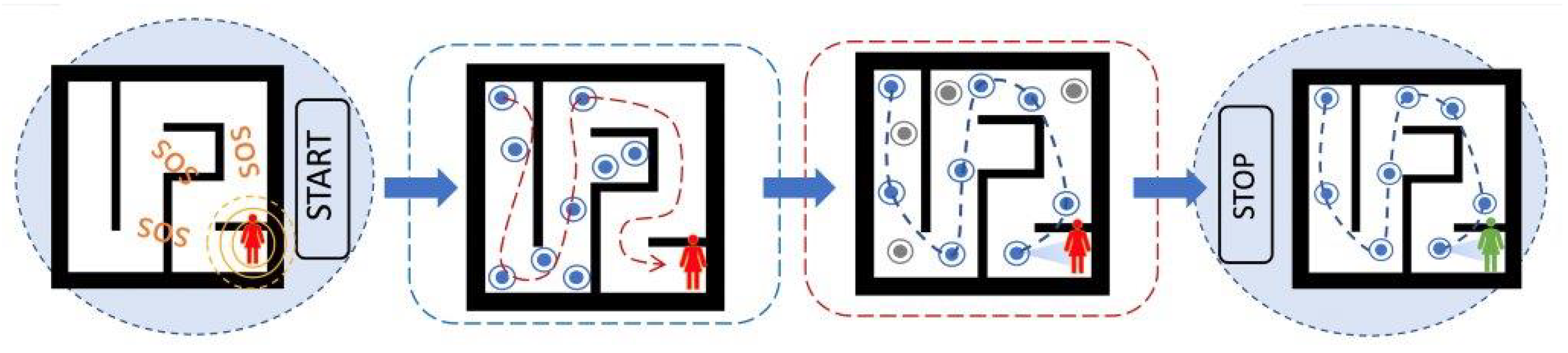
Figure 20.
A summary view of the SAR process in two phases. The search starts with a victim being trapped in the maze-like environment, broadcasting an SOS signal. In Phase-I, the search agents explore the environment in search of the SOS signal, using iAA algorithm. After locating the source of SOS signal, the agents switch to Phase-II, and find the shortest routing path to communicate information about the victim’s location to the base station. The remaining unused agents (marked in gray) can return to the base station.
Table 1.
Research in the field of deterministic and heuristic path planning strategies in maze-like environments, including Ant Colony Optimization (ACO), Particle Swarm optimization (PSO), and others. LP stands for Local Planning, HT stands for Heuristic Technique.
Table 1.
Research in the field of deterministic and heuristic path planning strategies in maze-like environments, including Ant Colony Optimization (ACO), Particle Swarm optimization (PSO), and others. LP stands for Local Planning, HT stands for Heuristic Technique.
| Ref | LP | HT | Algorithm Used |
|---|
|
[78] | | ✓ | Improved ACO |
| [79] | ✓ | | Artificial Potential Field Method |
| [80] | ✓ | ✓ | Multi Pheromones for tracking targets |
| [81] | ✓ | ✓ | Improved ACO Heuristic Function |
| [82] | | ✓ | Simple ACO |
| [83] | ✓ | ✓ | Repellent Pheromone for coverage |
| [84] | ✓ | ✓ | Advanced PSO |
| [85] | | ✓ | Genetic Algorithm with ACO |
| [86] | | ✓ | Hybrid ACO w. Random- + RL based-Search |
| [87] | ✓ | | Point Bug Algorithm |
| [88] | ✓ | | Dijkstra Algorithm |
| [89] | ✓ | ✓ | Fuzzy Logic with Counter ACO |
| [90] | | ✓ | PSO in partially known environments |
| [91] | ✓ | ✓ | Combination of multiple pheromones |
Table 2.
Research using deterministic and heuristic path-planning strategies; (✓) indicates maze-like environments with obstacles. The used algorithms are Dijsktra (D), Floyd-Dijsktra (FD), Ant Colony Optimization (ACO); others refers to a combination of sweep and savings.
Table 2.
Research using deterministic and heuristic path-planning strategies; (✓) indicates maze-like environments with obstacles. The used algorithms are Dijsktra (D), Floyd-Dijsktra (FD), Ant Colony Optimization (ACO); others refers to a combination of sweep and savings.
| | Reference | Cost Function | Alg. |
|---|
| ✓ | [93] | Distance, Gas Concentration | D, ACO |
| | [96] | Energy | D |
| | [97] | Distance | D |
| ✓ | [98] | Energy, Difficulty, Distance | D |
| ✓ | [99] | Distance | FD |
| ✓ | [100] | Distance | D, ACO |
| ✓ | [101] | Distance | D + others |
Table 3.
Dimensions and average complexities of the 5 maze types used in simulations; see
Figure 11.
Table 3.
Dimensions and average complexities of the 5 maze types used in simulations; see
Figure 11.
| | Dimensions | Complexity |
|---|
|
Maze 1 (M1) | 27 × 27 | 22 |
| Maze 2 (M2) | 39 × 39 | 47 |
| Maze 3 (M3) | 51 × 51 | 81 |
| Maze 4 (M4) | 63 × 63 | 129 |
| Maze 5 (M5) | 75 × 75 | 210 |
Table 4.
Cost estimates for all different possible directions/actions of movement.
Table 4.
Cost estimates for all different possible directions/actions of movement.
| Direction | Cost |
|---|
| Hover | 0.5 |
| Forward | 1 |
| 90 turn | 1.5 |
| Backward | 2 |


 ,
, 


