Abstract
This paper presents a time- and cost-efficient method for the management of construction and demolition (C&D) debris at construction sites, demolition jobsites, and illegal C&D waste dumping sites. The developed method integrates various drone, deep learning, and geographic information system (GIS) technologies, including C&D debris drone scanning, 3D reconstruction with structure from motion (SfM), image segmentation with fully convolutional network (FCN), and C&D debris information management with georeferenced 2D and 3D as-built. Experiments and parameter analysis led us to conclude that (1) drone photogrammetry using top- and side-view images is effective in the 3D reconstruction of C&D debris (stockpiles); (2) FCNs are effective in C&D debris extraction with point cloud-generated RGB orthoimages with a high intersection over union (IoU) value of 0.9 for concrete debris; and (3) using FCN-generated pixelwise label images, point cloud-converted elevation data for projected area, and volume measurements of C&D debris is both robust and accurate. The developed automatic method provides quantitative and geographic information to support city governments in intelligent information management of C&D debris.
1. Introduction
With the largest concrete consumption in the world in 2019, China has been generating an increasing amount of construction and demolition (C&D) debris as a result of construction, renovation, and demolition activities [1,2], the majority of which, however, has been landfilled or illegally dumped, causing adverse environmental impacts on the soil and water. Despite local investigations and regulations, such disposal and illegal dumping continue to exist due to the lack of automatic C&D identification and volume calculation tools. Therefore, we propose an automated method for C&D debris management at construction and demolition jobsites, landfill sites, and illegal dumping sites, which utilizes drone photogrammetry, deep learning, and geographic information system (GIS) in C&D debris surveying, detection, measurement, and information management. In addition, concrete debris detection and quantification experiments were conducted on an illegal dumping site, and the application benefits of the new method are discussed and summarized here. The method developed in this study provides quantitative and geographic information to support city governments and the related departments in C&D debris intelligent information management.
2. Background
2.1. Construction and Demolition Debris Management
Global cement production was estimated at approximately 4.1 billion tonnes (BT) in 2019 by the European Cement Association [1]. This huge amount of cement products indicates that the construction industry consumed a total of 27.4 billion tonnes (BT) of concrete worldwide in 2019, with approximately 15.4 BT in China, 1.2 BT in the EU, and 0.6 BT in the USA (note that in this calculation, concrete is assumed to be made of 15% cement, 75% aggregate, and 10% water) [1,2,3]. To meet such demand in China, its cement production increased from 1.08 BT to 2.3 BT from 2005 to 2019, while cement production has decreased in developed countries, dropping from 0.25 BT to 0.18 BT in the EU and from 0.1 BT to 0.09 BT in the USA between 2005 and 2019 [1,2]. On the other hand, while the amount of construction and demolition (C&D) waste has remained stable in developed countries, it has increased substantially in China due to construction, renovation, and demolition activities in residential, non-residential, and civil infrastructure projects. For example, approximately 0.85 BT of C&D waste was generated in the EU in 2012 (34% of total waste) compared with 0.83 BT in 2018 (36% of total waste) [4,5], whereas in China, it doubled from an estimated amount of 1.54 BT in 2005 to 3.53 BT in 2013 [6,7,8].
The material composition of C&D waste is mostly concrete, metal, mortar, brick/block, plastic, and timber, where concrete debris typically contributes the largest percentage (60% by weight), followed by brick (21%) and mortar (9%) [7,9]. In developed countries, much of this waste is reused; for example, 76% of C&D debris was processed for further use in the USA, and most concrete debris was recycled into aggregates or new concrete products [10]. On the contrary, China has a rather low C&D debris reselling and recycling ratio of 8%, indicating that 92% of concrete, brick, and mortar waste is landfilled [9]. This is partially because the potential recycling values of concrete, brick, and mortar in China are only 4% of the recycling value of metal, which is relatively low compared with other developing countries, e.g., 10.4% in Bangladesh [8,9]. Moreover, to further reduce the transportation and landfill cost of C&D waste, much of the concrete debris is dumped at illegal sites, imposing substantial environmental impacts on the soil, surface water, groundwater, and air quality after long-term sun exposure and saturation by rain.
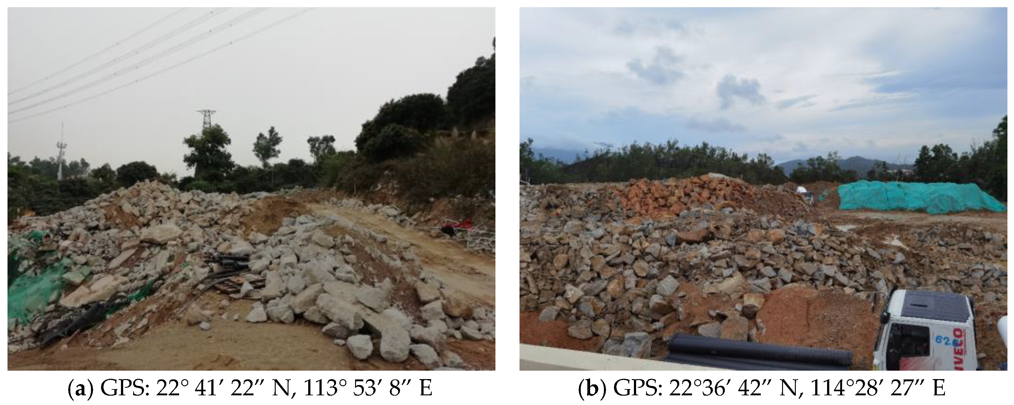
Figure 1 shows the conditions of two illegal dumpling sites in Shenzhen, China, captured by an engineer of the local construction waste management team during a field visit. In Shenzhen, the identification and investigation of C&D waste is conducted via field visits and on-site measurements, which are time- and labor-consuming to achieve satisfactory results. In addition, illegal dumping sites are typically located in rural and mountainous areas, where access to the waste stockpile is limited and the soft soil surfaces also create safety hazards of sliding and falling debris. Such barriers greatly hinder the construction waste management team’s ability to accurately measure the quantities of C&D debris, impacting the decision making of subsequent transporting and cleaning tasks. Although the local regulation “Shenzhen Construction Waste Management Method” specifies the punishment for illegal dumping, it does not differentiate the severity of violations such as dumping areas and volumes [11]. As a result, illegal dumping of C&D waste continues to exist in Shenzhen, China. Therefore, it is necessary and urgent to employ an automatic construction waste stockpile measurement tool for the construction waste management team to efficiently identify C&D waste quantities and accurately issue citations based on measurable individual violations.
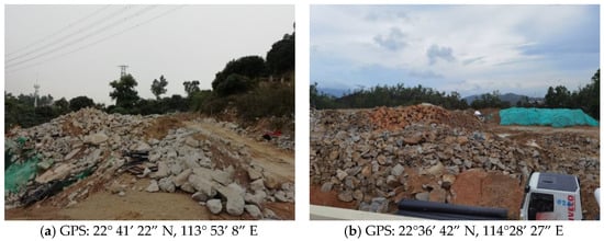
Figure 1.
(a,b) Illegal construction waste dumping sites in Shenzhen, China (Images by authors).
2.2. Literature Review
Previous research deployed remote sensing (RS) technologies in construction waste management, such as satellite imagery. The benefit of its extensive areal coverage and feasibility has been demonstrated in illegal landfill detection [12,13], monitoring the surface temperatures of municipal solid waste landfill sites [14], and volume estimates of stockpiled reclaimed asphalt pavement inventory [15]. However, the resolution of typical satellite imagery limits its application in investigating scattered C&D waste illegal dumping sites in urban, suburban, and rural areas. To obtain high-resolution aerial images, drones and cameras are a potential solution that has been successfully applied in 3D mapping and surveying [16,17,18,19,20,21], building and infrastructure structure inspection [22,23,24,25,26,27], and search and rescue applications [28,29,30]. Furthermore, the advancement of structure from motion (SfM) photogrammetry has made it possible for convenient aerial image-based 3D reconstruction with ready-to-fly consumer drones, e.g., DJI Mavic 2 Pro (SZ DJI Technology, Shenzhen, China), which can achieve high accuracy within 5 cm error in both horizontal and vertical coordinates [16,31,32], and the obtained point cloud can be used in soil volume estimation [17,32,33].
Furthermore, with the advancement of deep learning technologies, e.g., convolutional neural network (CNN)-based image classification and fully convolutional network (FCN)-based image segmentation, automated object detection has become more convenient and accurate in images no matter the target objects’ sizes and shapes [22,25,34,35,36,37,38,39,40,41]. Researchers have conducted several studies in waste image classification and waste material detection, including municipal solid waste and construction waste, which were separated as “eyes” and a “brain” in domestic waste automatic sorting machines and construction waste recycling robots (see Table 1). These previously developed approaches are all CNN-based image classification methods, which are suitable for extracting one target object from a small image (equivalent to multiple target objects in a large image).

Table 1.
Waste classification and waste material detection via deep learning.
However, for extracting stockpiled C&D materials, e.g., concrete debris, from drone imagery, FCN-based image segmentation is required, where all pixels belonging to concrete debris are expected to be assigned a corresponding class label, as in [22,42]. The image segmentation results will help estimate the projected area of concrete stockpiles if the ground sampling distance (GSD) is known for the drone images and also can be used for stockpile volume estimation if the images’ elevations are known.
3. System Design and Development
3.1. System Overview
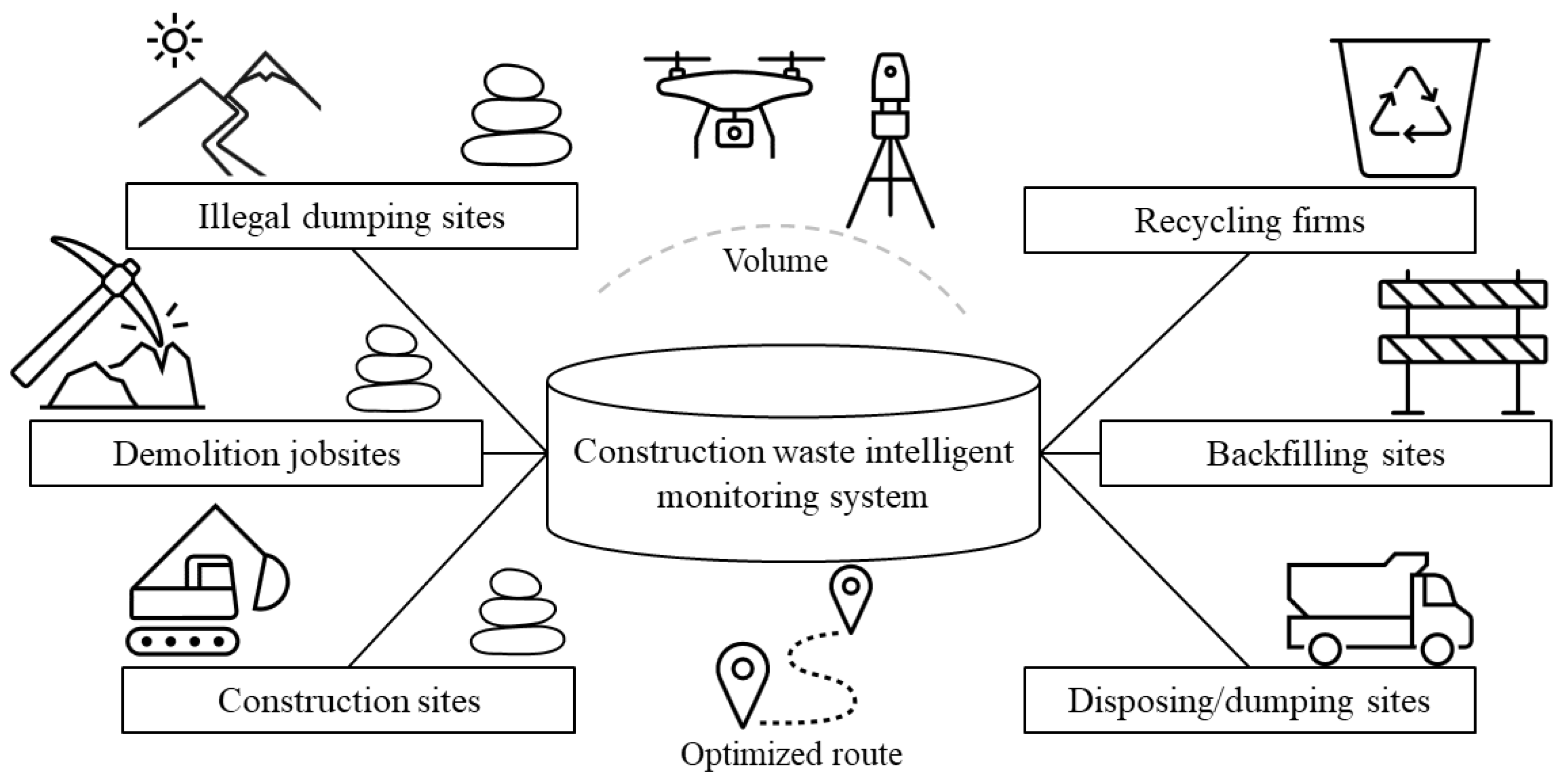
To facilitate construction waste management and alleviate related environmental concerns, we propose a time- and cost-efficient method that integrates drone photogrammetry, deep learning, and GIS to automate the process of C&D debris identification and measurements at construction and demolition jobsites, landfill sites, and illegal dumping sites, as illustrated in Figure 2.

Figure 2.
Enhanced construction waste intelligent information management system.
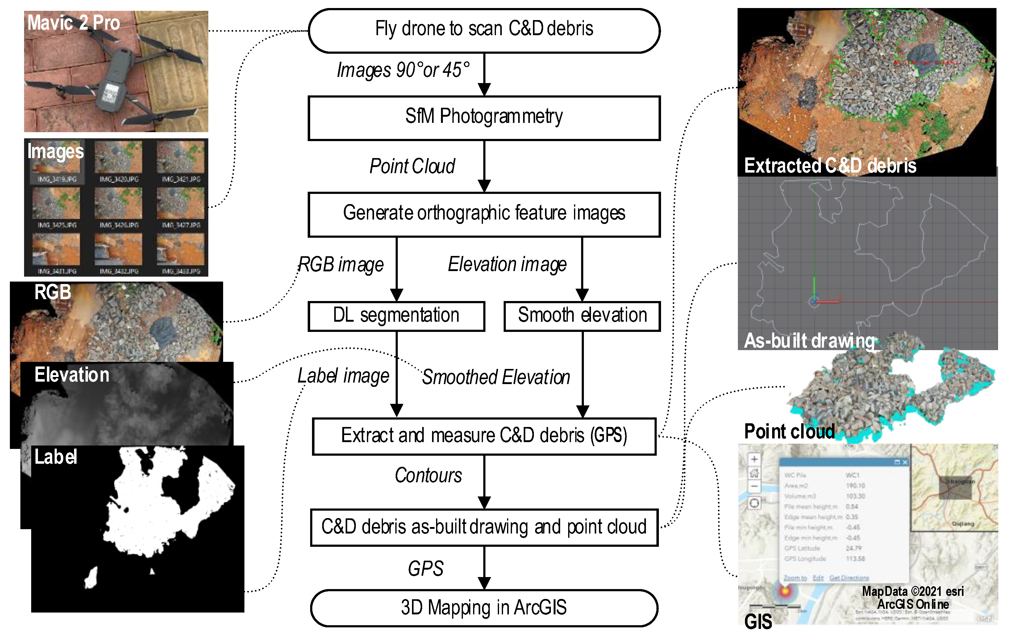
Figure 3 presents the overall process used in the proposed automated method for C&D debris detection, measurement, and documentation, which are explained using waste concrete debris (written as WC for the remainder of the paper), including C&D debris scanning, SfM photogrammetry, point cloud RGB texture and elevation feature image generation, deep learning-based segmentation, and C&D debris extraction, measurement, as-built modeling, and GIS mapping.

Figure 3.
Proposed workflow. (Images by author. Map Data © 2021 esri.)
3.2. Aerial Image Collection and Photogrammetry
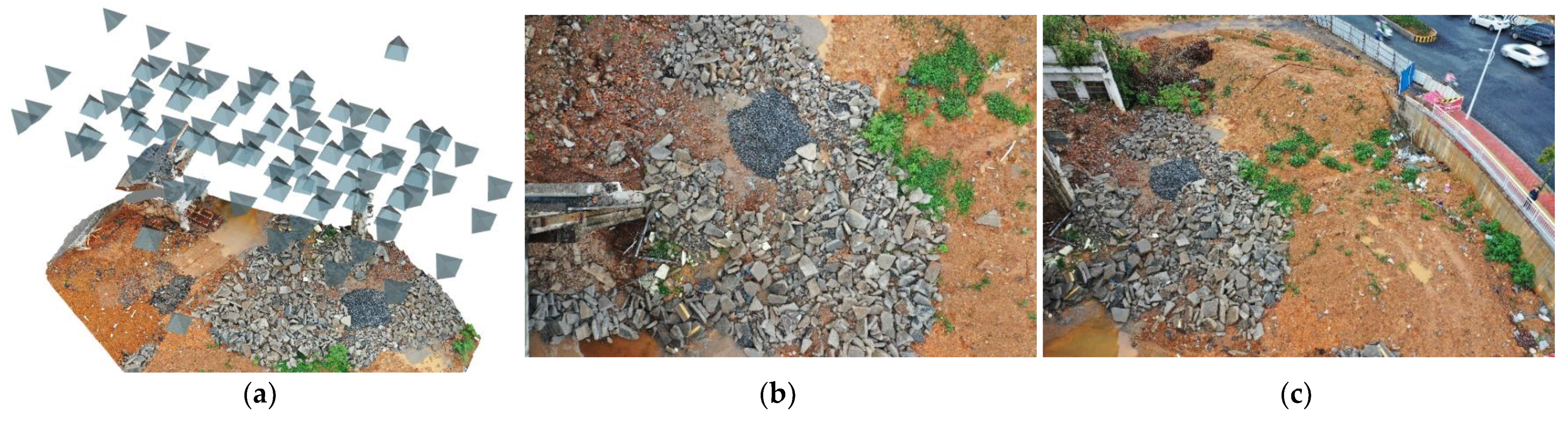
To enhance the SfM photogrammetry performance, the following scanning strategies are recommended in aerial image collection: (1) on a forward path, set the drone gimbal’s pitch axis at negative 90° to make the camera lens face the ground for capturing overlapped top-view images of C&D debris (stockpiles), such as those shown in Figure 4b; (2) on a backward path, set the pitch axis at negative 45° to capture side-view images of the C&D debris (stockpiles), as shown in Figure 4c; and (3) hover above the center of each of the scanned C&D stockpiles to capture additional top-view images for global positioning system (GPS) information collection.
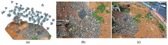
Figure 4.
Aerial images: (a) camera pose, (b) 90° image, and (c) 45° image.
Following that, we can import the captured 90° and 45° images into SfM photogrammetry software, such as Autodesk ReCap Photo (Autodesk, Mill Valley, CA, USA), to generate a 3D mesh model (Figure 4a) and a 3D point cloud for the scanned site.
3.3. Point Cloud Feature Image Generation
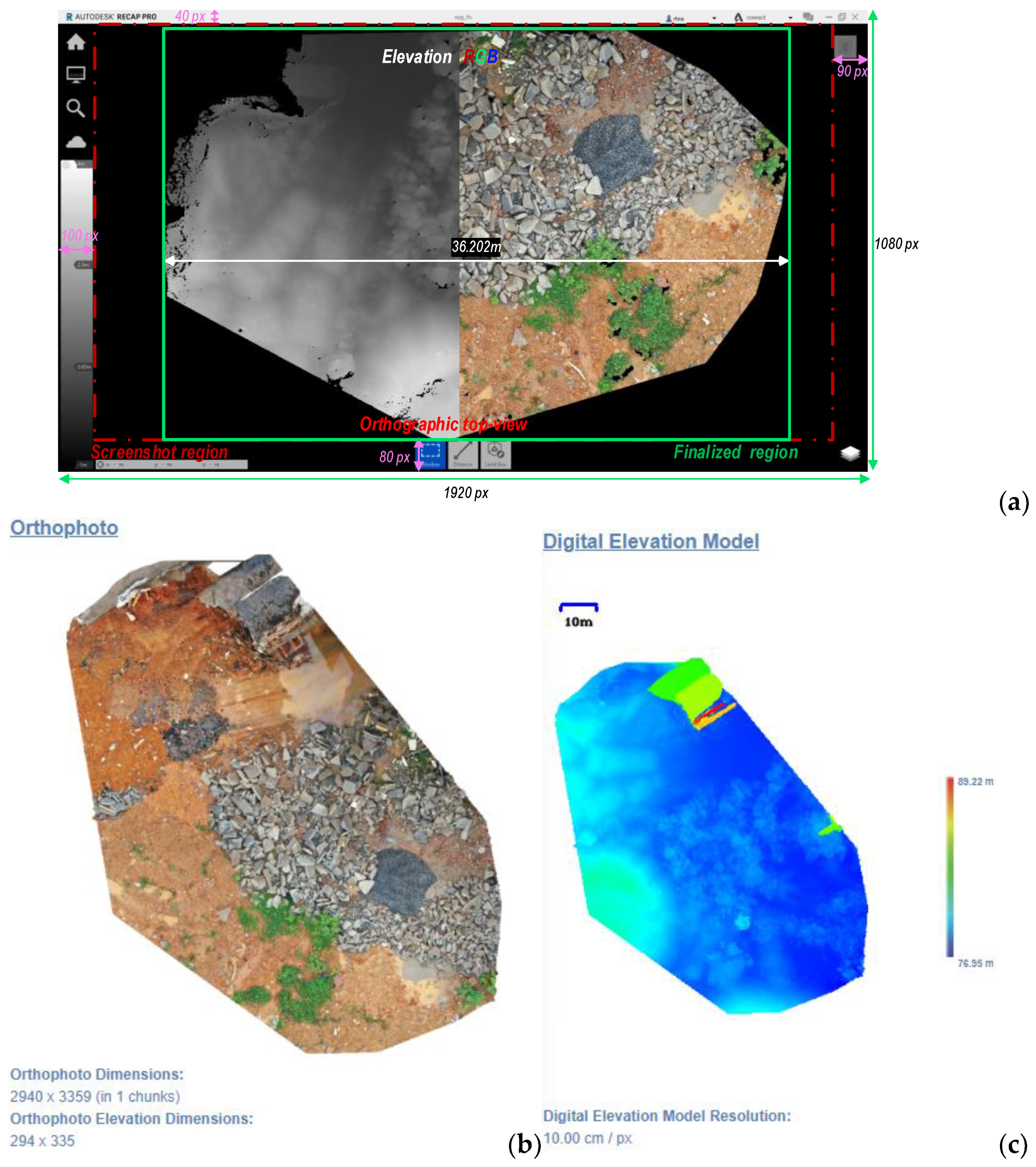
Orthophoto and digital elevation model (DEM) images can be generated from photogrammetry software, i.e., ReCap Photo. The resolution of the DEM image, however, is only one-tenth of the orthophoto, with, for instance, pixel dimensions of 294 × 335 compared to 2940 × 3359, respectively, as demonstrated in Figure 5c,b. The low resolution of the DEM image makes it difficult to accurately register elevation data to each RGB pixel in the orthophoto. Fortunately, each point in photogrammetric results has multiple attributes, e.g., “RGB” and “elevation”, which can be visualized using different views, scales, and colors in point cloud visualization and editing software. As a result, Autodesk ReCap Pro (Autodesk, Mill Valley, CA, USA) was used to generate RGB texture and elevation feature images for point clouds. For example, in Figure 5a, the “RGB” (red, green, blue) option displays points with camera-captured colors, while the “elevation” view represents each point’s height in Z-coordinates [43]. Once the perspective mode is turned off, the orthographic top-view of an RGB point cloud in Figure 5a is similar to a large-sized orthophoto in Figure 5b, and the top-view of an elevation point cloud in Figure 5a is similar to a DEM in Figure 5c. By setting the same scale, the orthographic top-view images of the RGB texture and elevation of a point cloud in ReCap Pro are originally linked to the same pixel coordinates, as shown in Figure 5a.

Figure 5.
Designed screenshot tool: (a) point cloud, (b) orthophoto, and (c) DEM.
Accordingly, we designed a screenshot tool to obtain the RGB (in 24-bit) and elevation (in 8-bit) images from ReCap Pro for deep learning model training and testing data set preparation with the following steps: (1) crop the 1080 p capture by removing the toolbars in each side of the capture, and (2) further remove the black margins on each side of the cropped capture to obtain the finalized region annotated in Figure 5a. The ground sampling distance (GSD) of the future images can then be determined via Equation (1).
where the is the width of the finalized region, such as the examples shown in Figure 3, and the can be accurately measured from ReCap as the ortho distance annotated in Figure 5a. In addition, a median filter [44] with a size of 11 × 11 pixels is proposed to smooth (replace) point gaps, shown as black in Figure 5a, to obtain a smoothed elevation image but maintain the edges of elevation changes.
Furthermore, we also developed a Pointcloud2Orthoimage (P2O) tool (code and demo on [42,45]) to automatically generate feature images of orthoimage and elevation images from a point cloud file. The generated feature images have unlimited size, which means any scanned large site can be presented in a single-frame, high-resolution image. Meanwhile, the differently sized RGB feature images also have the same GSD.
3.4. Pixelwise Segmentation Models and Label Image Generation
In this research, two deep learning models (FCNs), a convolutional encoder-decoder network (Table 2) and a U-Net [46], are compared for WC (label = 255) and non-WC (label = 0) binary segmentation. Previous studies showed that the U-Net [47] can be implemented with a Sigmoid activation function using two integers of 0 and 1 to achieve suitable performance in binary classification for different shaped and sized AEC objects [22]. Thus, we used the Sigmoid function in the end layer of the encoder-decoder as well. Following that, the one-channel pixelwise label image has a pixel value range of 0 to 255 after multiplying by 255 the Sigmoid results, which are in the range of 0 to 1. In addition, the encoder-decoder only uses three max pooling layers and three up-sampling layers to ensure the label image outputs have the same dimensions as the ortho-image inputs. Hence, the encoder-decoder is lighter (has much fewer layers, channels, and parameters) than the U-Net, and more likely to be implemented by a video card (GPU) with fewer CUDA cores.
Table 2.
Convolutional encoder-decoder network model layers.
Since directly processing a large image requires more memory in a single GPU, we applied a disassembling and assembling algorithm [48] for both model training and prediction stages. In detail, a large image was first disassembled into multiple small patches with dimensions of 128 × 128 pixels, each of which overlapped 50% with adjacent small patches in both width and height directions. Then, for each large image, FCNs processed the disassembled small patches rather than directly processing the full-resolution input image. The FCNs then generated small-patch outputs that were assembled to produce a label image with the same dimensions as the high-resolution input RGB image. Consequently, with the 128 × 128-pixel small patch as the input, the proposed encoder-decoder model only has 1,330,305 parameters, while the complicate U-Net has 23.33 times more parameters (31,032,837). As a result, the proposed FCN-based pixelwise segmentation method can be run on a workstation with a Core i7-7800X CPU@3.5 GHz, 32GB RAM, and 11GB GDDR5X memory GeForce GTX 1080 Ti GPU for pixelwise label image generation for large-sized inputs.
Moreover, we propose the following data augmentation (DA) strategies in preparing the 128 × 128-pixel RGB image and label image samples. (1) Randomly flip the image and label in one of the following options: horizontal, vertical, both horizontal and vertical, or non-flipped. (2) Randomly uniformly resize the flipped image and label by a factor in the range of [0.5, 1.5]. (3) Randomly rotate the resized image and label in the range of [1, 89] degrees (note that the resized image and label were padded with sufficient black margin, i.e., 0 values, prior to rotation to retain all relevant textured regions). (4) Either randomly conduct perspective transformation of the image and label (keep left, right, top, or bottom edge the same) or not. (5) Cut the black margins (i.e., left, right, top, and bottom edges) from the transformed image and label. (6) Pad the remaining image and label with 0 values to be multiples of 128 pixels in size. (7) Randomly adjust the padded image’s brightness, color, contrast, or sharpness by a value in the range of [0.5, 1.5] [49] (note that adjustments are not applied to the label). (8) Rotate the adjusted image and label by 0°, 90°, 180°, and 270° (when combined with step (2), this covered nearly all possible 360° rotations). (9) Crop the four sets of rotated images and labels into 50% overlapped 128 × 128-pixel small patches by moving a 128 × 128-pixel slide window with a stride of 64 pixels in both width and height directions. (10) Discard black image and label samples, i.e., all pixels with a value of 0, for reducing the overall size of training data sets. Consequently, well-trained image segmentation models can be obtained under the condition of limited model training data sets.
3.5. C&D Debris Extraction, Measurement, Modeling, and Mapping
We used the function [50] to extract the contours of all individual C&D debris (stockpiles) that occurred in a pixelwise label image and return a list of contours, irrespective of their sizes (measured in pixel area). This meant that the fragile debris was also included in the return list. Thus, an area filter of 10,000 pixels was used to skip thin debris as noise. An example of an extracted contour is shown in Figure 3, which is the boundary of a WC stockpile. Each contour’s vertices’ local pixel coordinates can then be transformed into real-world coordinates via Equation (2):
where and set the origin of the customized real-world coordinates at the image center. Alternatively, the origin location can be set at a known ground control point. and are the minimum and maximum elevation values of the elevation image in the range of [0, 255], in which corresponds to a grayscale value of 255 and is equivalent to a grayscale value of 0. Thus, when assuming C&D debris are evenly distributed across the base area and along the stockpile height, the projected area and volume of C&D debris can be estimated using Equations (3a) and (3b):
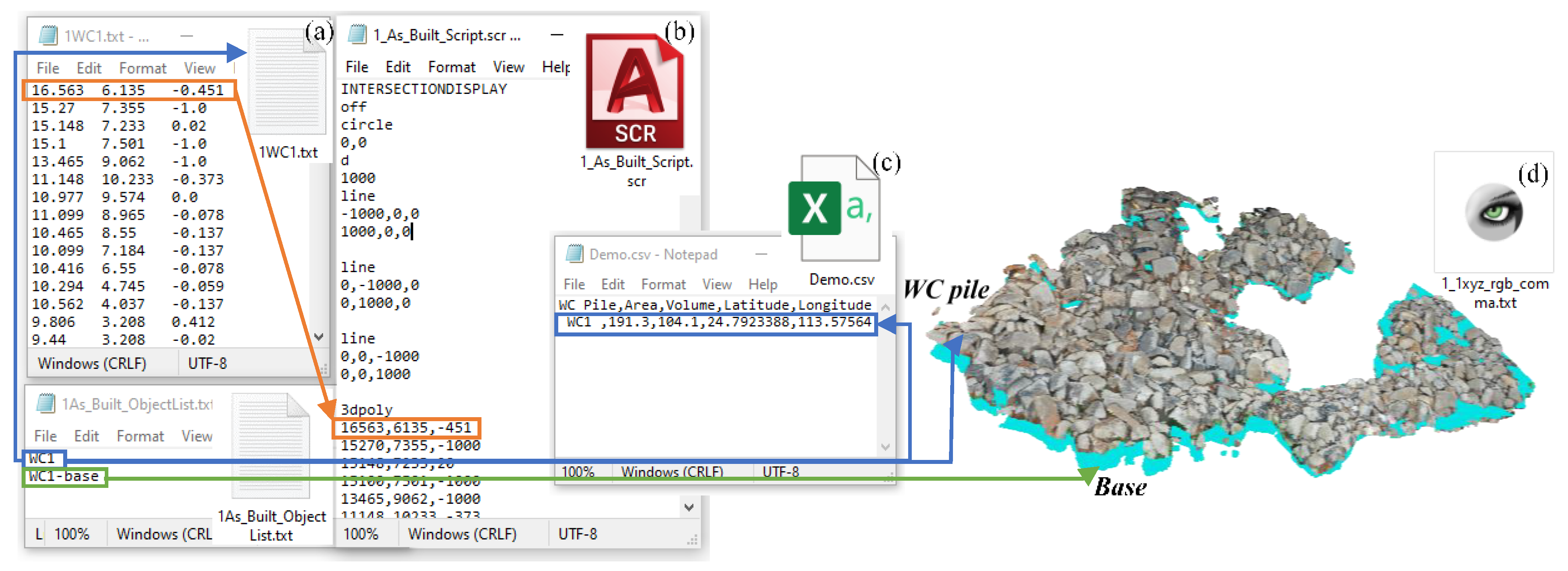
where is the mean elevation value of the contour enclosed region of the smoothed elevation image. When the ground surface is a flat plane and the customized origin is set on that plane, the is equal to zero. Alternatively, the can be set as the mean elevation value of the boundary of the C&D debris area. The estimated geometry data are saved in a comma-separated value (CSV) file (Figure 6c) along with the extracted GPS data, which was imported into ArcGIS Online (Esri Redlands, California) for geographic visualization and information management. The converted real-world coordinates (units in meters) of each extracted C&D debris area are initially saved in text files (Figure 6a) and then converted to a single script file (Figure 6b) (units in millimeters) for automatic drawing in Autodesk AutoCAD/Civil 3D (Autodesk, Mill Valley, CA, USA) like in [45]. Furthermore, a C&D debris stockpile point cloud file (Figure 6d) is produced by using all C&D pixels of the RGB image and elevation image, and the same output is also generated for the projected stockpile’s base, as shown in Figure 6d.

Figure 6.
Data relationships: (a) counters and coordinates, (b) CAD script, (c) CSV file, and (d) point cloud file.
4. Experiments and Results
4.1. Experimental Site and Data Set Preparation
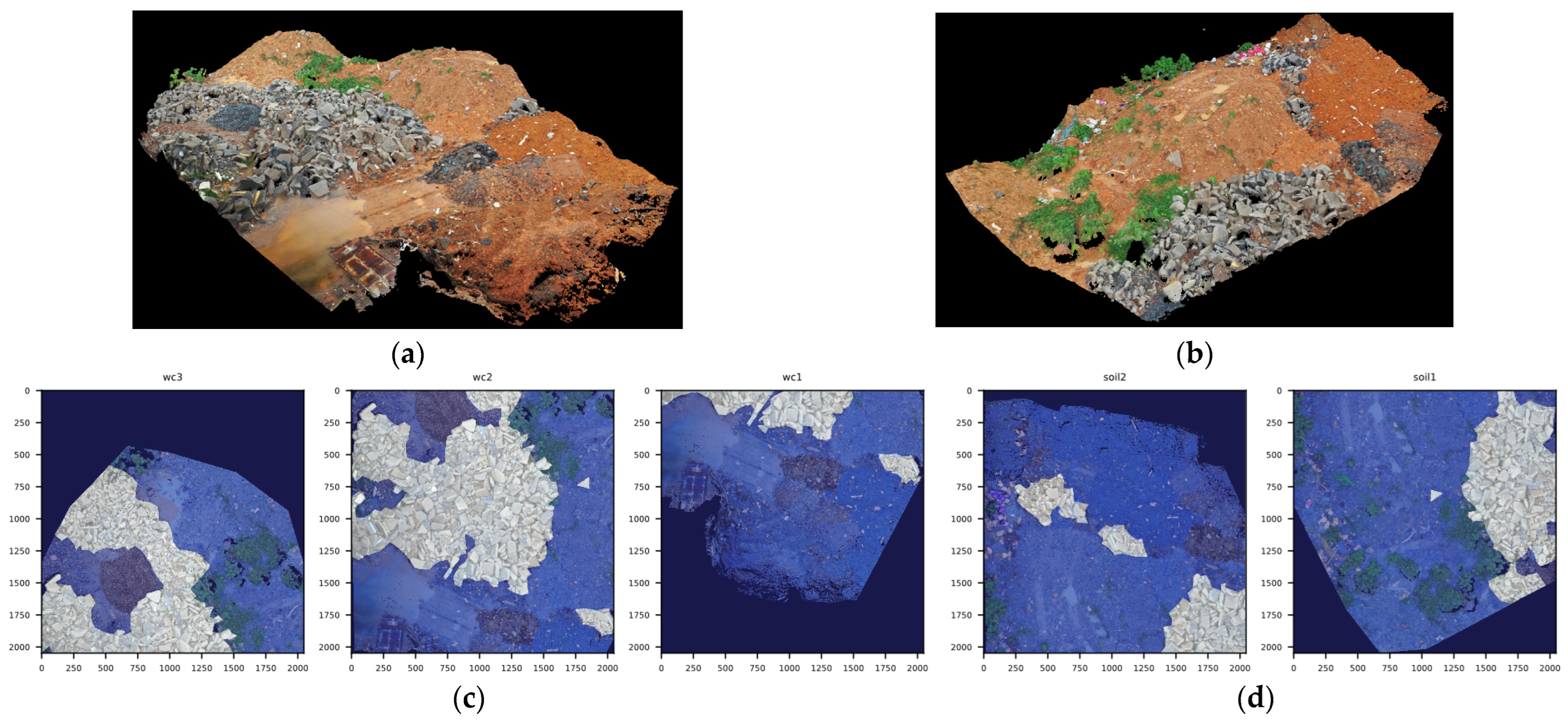
An illegal C&D waste dumping site (Figure 4), which was previously an abandoned industrial building in Shaoguan, China, was selected for experiments. As shown in Figure 1, Figure 4 and Figure 7, typically only a single material category exists in a stockpile because truck drivers want to quickly complete their illegal dumping behaviors. As a result, it is their best choice to dump at a clear site without any previously dumped C&D debris. Thus, it is reasonable to assume that the composition of C&D debris was evenly distributed across the area and elevation of the stockpile. Two sets of aerial images were collected from 14 to 15 April 2021 with a Hasselblad L1D-20c aerial camera (1” CMOS, F/2.8, 20 megapixels) via a DJI Mavic 2 Pro drone (SZ DJI Technology, Shenzhen, China). We manually controlled the drone to hover over the site at altitudes of 10 m, 20 m, and 40 m to capture images. Two point clouds were then generated via ReCap Photo, as shown in Figure 7a, which focused on a WC stockpile, and Figure 7b, which mainly covered a soil stockpile. The two point clouds were separately imported into ReCap Pro to export two sets of RGB images (in orthographic top-view), including three 2048 × 2048-pixel RGB images (Figure 7c) for model training and two 2048 × 2048-pixel RGB images (Figure 7d) for testing. The exported images are similar to the orthophoto but have gaps among points due to the nature of the source point cloud, whereas the orthophotos are continuous photographic images without gaps. Following that, the 2048 × 2048-pixel label images (see Figure 7c,d) were manually created by annotating WC pixels with a value of 255 and non-WC pixels with a value of 0. The data sets are available in [45].
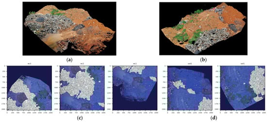
Figure 7.
Data sets: point cloud (a) WC stockpile, (b) soil stockpile, (c) training data, and (d) testing data.
4.2. Image Segmentation Model Training, Testing and Comparison
4.2.1. Model Training
Both FCNs were set up using Keras 2.3.1, Python 3.6.8, OpenCV 3.4.2, and TensorFlow-GPU 1.14 software packages, and run on a workstation with 2 × Xeon Gold 5122@3.6GHz CPUs, 96GB DDR4 2666 MHz memory, and 4×11GB GDDR6 memory GeForce RTX 2080 Ti GPUs for model training. In model compiling, the encoder-decoder applied the Keras settings of optimizer = ‘rmsprop’ and loss = ‘mse’, and the U-Net applied the settings of optimizer = ‘adam’ and loss = ‘binary_crossentropy’. In addition, the following common configurations were set for model training and validation: (1) callbacks = [EarlyStopping(monitor = ‘val_loss’, patience = 10)] to avoid model overfitting, which stops model training when the validation loss does not decrease for 10 epochs; (2) epochs = 100, which stops model training at the 100th epoch; and (3) validation_split = 0.05, which uses 5% of samples for validation during model training.
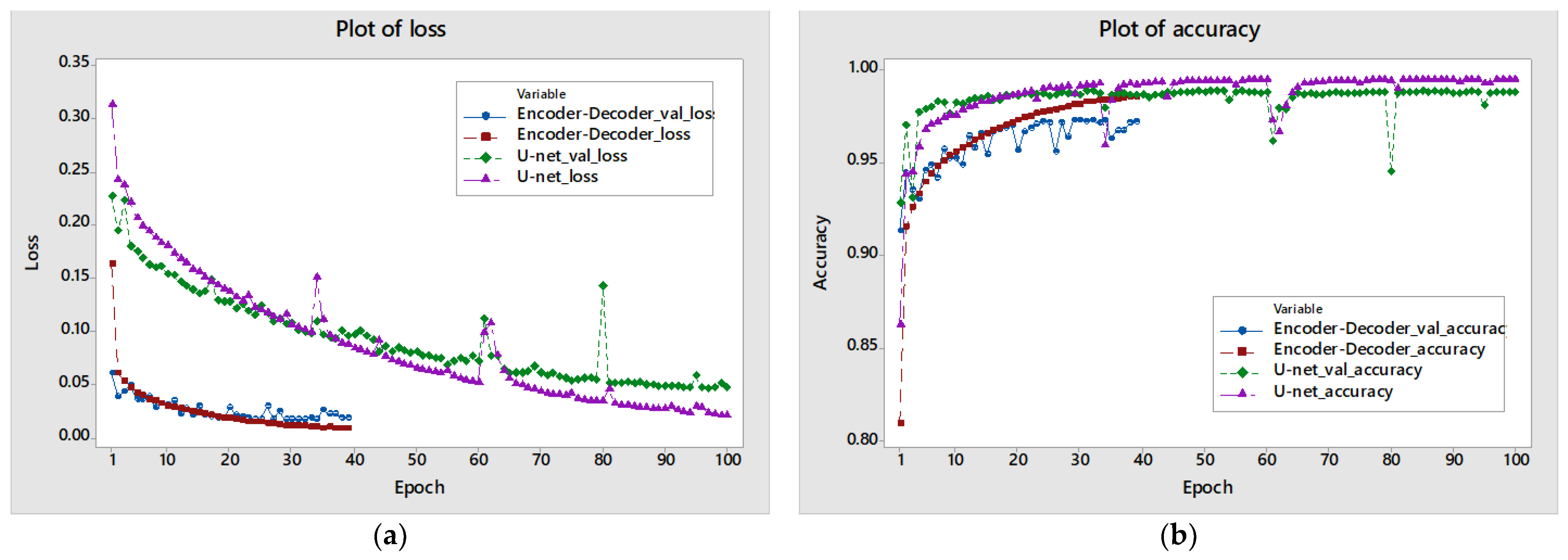
By performing 11 rounds of the 10 steps in the combined data augmentation (DA) process (which skips random processing steps (1) to (4) and (7) in the first round to keep the original image and label, and then runs all steps for the remaining rounds), the created model training data sets would have sufficient size, shape, color, orientation, and perspective differences to characterize a range of WC and soil stockpiles. As the DA was randomly conducted in model training, the encoder-decoder was trained on 80,071 samples and validated on 4215 samples, and the U-Net was trained on 74,725 samples and validated on 3933 samples by the setting of validation_split = 0.05. The plots of training and validation loss and accuracy are shown in Figure 8. The encoder-decoder terminated early (at the 39th epoch) with a training loss value of 0.0087 and accuracy of 0.9852, and a validation loss of 0.0182 and accuracy of 0.9719. The U-Net training was completed at the 100th epoch (i.e., the early stopping function was not activated as its criteria was not met) with a training loss of 0.0210 and accuracy of 0.9949, and validation loss of 0.0477 and accuracy of 0.9878.
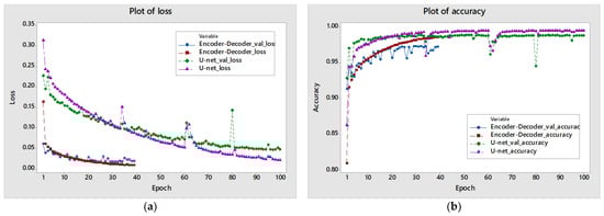
Figure 8.
Plots of (a) loss and (b) accuracy.
The U-Net training typically took 159–162 s for each epoch on the four-GPU workstation, while the encoder-decoder averaged 45 s for each epoch. This is reasonable given that the U-Net has more layers and parameters than the proposed encoder-decoder (Table 2). For future practice, using the simple encoder-decoder would be a fast implementation option when new data sets (image and label image) should be prepared, and new FCN should be trained for the detection of other C&D materials.
4.2.2. Model Testing
Since the Sigmoid activation function was used in both FCNs to generate the continuous values in the range of 0 to 1, we multiply by 255 to produce continuous values in the range of 0 to 255 for the pixelwise label image. Hence, a filter is necessary to classify pixels into two groups, the WC pixels and non-WC pixels, as the binary segmentation results. In this research, for both FCNs, all pixels with a value >127 were updated to 255 to indicate WC; otherwise, they were replaced with 0 to represent non-WC objects. In addition, previous research showed a filter that replaces a pixel prediction that falls in the range of (class-label−15, class-label+15), and the defined value of each class label can yield adequate performance in multiclass segmentation tasks [48]. Thus, the following alternative option was tested for the encoder-decoder: all pixels within the [0, 15] range were updated to 0 for non-WC, and all values within the [240, 255] range were updated to 255 for WC.
Both trained FCNs were used to segment the five large-sized RGB images in Figure 7 using the disassembling and assembling algorithm, and the evaluation results of pixel accuracy, WC intersection over union (IoU), and Non-WC IoU values are compared in Table 3 for both training and testing data sets. By updating all pixel predictions with values >127 to 255 to indicate WC objects and replacing others with 0 to represent non-WC objects, the two FCN models generated similar results of IoU performance in the training data sets of wc3 and wc2 and the testing data set of soil1. In addition, Table 3 shows that the maximum WC IoU difference value between the U-Net and the encoder-decoder is only 0.0473 for training data set wc1 and 0.0844 for testing data set soil2. This is much better than the alternative option, which has a WC IoU difference of 0.0612 in data set wc1, and a difference of 0.1057 in data set soil2.
Table 3.
Training and testing evaluation results.
Furthermore, the assembled large image label predictions are shown in Figure 9, where the encoder-decoder mislabeled several WC areas are in the left side of testing data set soil2 (Figure 9d) compared to the U-Net prediction (Figure 9c) and the ground truth label image (Figure 7d). The mislabeled objects are plastic bags, which have a similar texture to concrete in the image. Due to its superior accuracy, the U-Net was used for the remaining applications. Table 3 shows that the pixel accuracy and IoUs of the training and testing data sets are very close to 1, but these slight differences cannot be further reduced by adding more training epochs due to the point gaps of the RGB images, which were filled with a WC label in the manually created label images but were successfully identified as non-WC objects in the assembled label image predictions. Moreover, the pixelwise segmentation results of the point clouds’ perspective views and orthographic oblique views are also shown in Figure 9e–h, where the U-Net successfully detected the WC stockpile and the scattered WC pieces, which confirmed the effectiveness of the proposed DA.
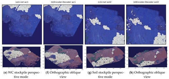
Figure 9.
Assembled label image prediction: U-Net results for (a) wc1 and (c) soil2; encoder-decoder results for (b) wc1 and (d) soil2; U-Net results for WC stockpile (e) perspective views and (f) orthographic oblique view; U-Net results for soil stockpile (g) perspective views and (h) orthographic oblique view.
4.3. Concrete Debris Extraction, Measurement, and Modeling
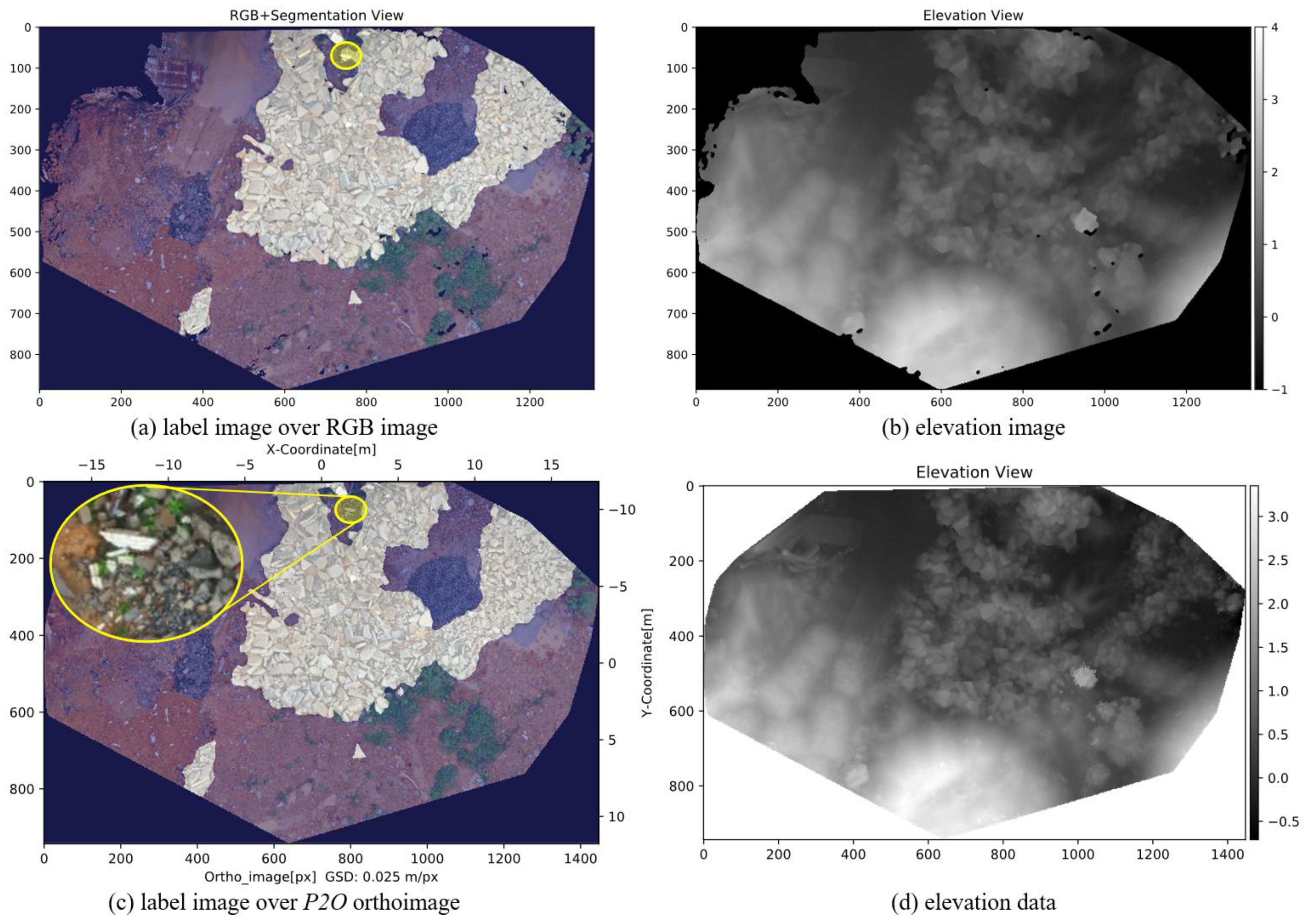
The target WC debris stockpile was placed in the center of the screen as in Figure 5 by zooming to extents, and the previously described screenshot tool collected the point cloud’s RGB and elevation image (see Figure 10) with an orthographic top-view from ReCap Pro, where the point display size was set at the default value of 2. The WC stockpile has a of 36.202 m (see Figure 5). The captured grayscale elevation image has an of 4 m and of −1 m, as shown in Figure 10b. The finalized RGB and elevation images have the dimensions of 1358 pixels in width and 886 pixels in height, which were automatically determined in the screenshot tool by dropping all black margins. Then, the GSD was calculated via Equation (1) as 0.026658321 m/pixel (36.202 m/1358 pixel). In addition, the P2O tool generated the orthoimage and elevation data shown in Figure 10c,d using the designated GSD = 0.025 m/pixel and elevation values in the range of −0.710394 m to 3.353387 m. The generated feature images have the size of 1448 × 944 pixels, and the = 0.025 × 1448 = 36.2 m, which is equal to the manually measured result of 36.202 m (see Figure 5).
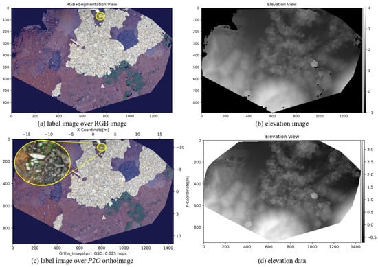
Figure 10.
WC stockpile segmentation and elevation data: (a) RGB image (with label) and (b) elevation image by ReCap Pro; (c) RGB image (with label) and (d) elevation image by P2O tool.
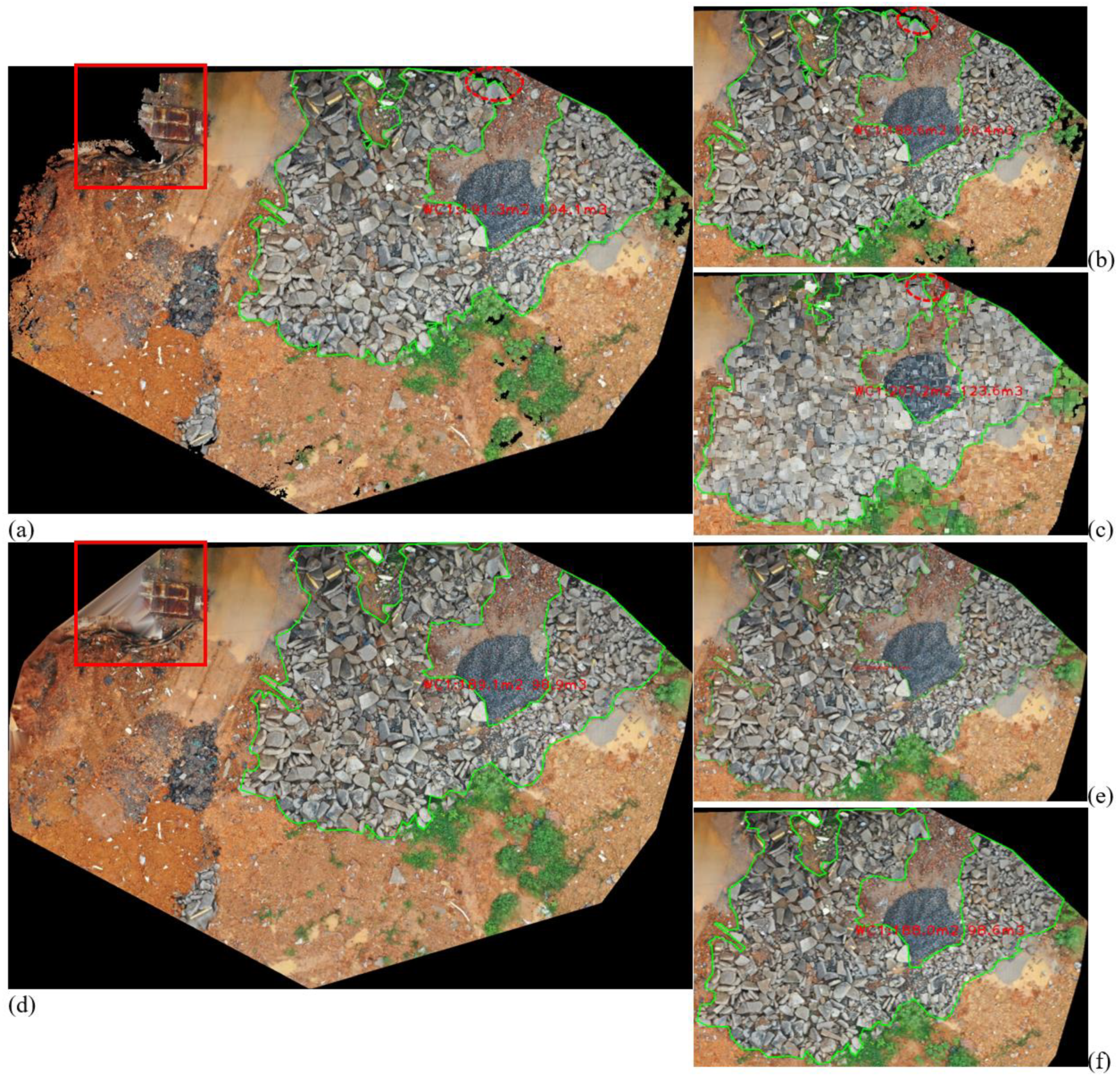
Consequently, the RGB image was dissembled into several 128 × 128-pixel small patches and then processed by the trained U-Net for 128 × 128-pixel label image prediction, and the large-sized pixelwise label image was assembled for WC stockpile extraction, as shown in Figure 10a. Once the contour of the WC stockpile was obtained, its projected area of 191.3 m2 and volume of 104.1 m3 were estimated using Equations (3a) and (3b). The extraction and measurement results are annotated in Figure 11a, where the scattered thin WC pieces and the small WC stockpile in the bottom-left were dropped by the 10,000-pixel area filter. In addition, the U-Net-generated label image for the P2O result is shown in Figure 10c. The major difference between Figure 10a,c is annotated and the detailed section is shown in Figure 10c as well. This section has pavement marks and aggregate particles mixed with thin concrete debris, and thus it is reasonable for the U-Net model to identify this region as non-WC. Following that, the extracted WC stockpile has a projected area of 189.1 m2 and a volume of 98.9 m3 in Figure 11d, which is slightly less than the 191.3 m2 in Figure 11a. The extracted WC stockpiles have a 1.15% = (100 − 189.1/191.3 × 100)% area difference, which is reasonable due to the U-net generating the different label images. However, the 5% = (100 − 98.9/104.1 × 100)% volume difference is unreasonably large and is discussed later.

Figure 11.
WC stockpile extraction: (a) point size = 2, area = 191.3 m2, volume = 104.1 m3 (red texts), (b) point size = 1, area = 188.6 m2, volume = 100.4 m3, (c) point size = 10, area = 207.2 m2, volume = 123.6 m3, (d) GSD = 0.025 m/pixel, area = 189.1 m2, volume = 98.9 m3, (e) GSD = 0.01 m/pixel, area = 189.8 m2, volume = 99.6 m3, and (f) GSD = 0.030 m/pixel, area = 188.0 m2, volume = 98.6 m3.
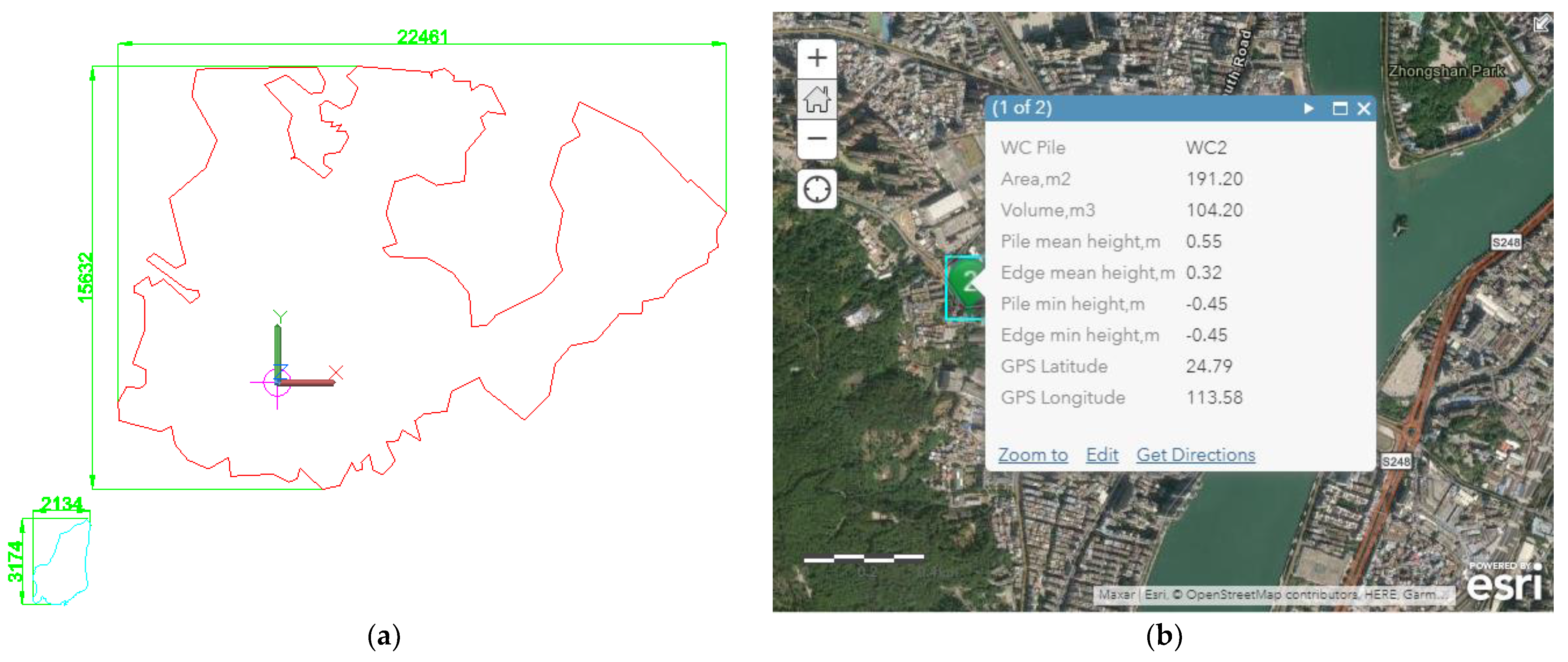
Additionally, the above processes were repeated to test the effect of filter size, where an area filter of 1000 pixels was applied to extract WC debris stockpiles from another captured and finalized RGB image with dimensions of 1357 × 886 pixels. Two WC stockpiles were extracted and modeled in CAD and ArcGIS Online, as shown in Figure 12. The larger one has an area of 191.2 m2 and a volume of 104.2 m3; these values are close to the results annotated in Figure 11a with the 10,000-pixel area filter. Thus, the developed method using photogrammetric point cloud-generated RGB and elevation images is a robust, accurate, and effective approach for WC debris volume estimation.
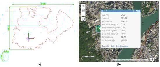
Figure 12.
WC stockpile modeling: (a) as-built drawing (unit, mm), (b) ArcGIS Online. (Map Data © 2021 esri.)
5. Discussion
5.1. P2O-Feature Image and GSD Parameter Analysis in Segmentation Performance
The performance of FCN-based image segmentation has a strong relationship with the comprehensive level of the model training data sets. The arbitrary view segmentation results in Figure 9e–h confirm that using only orthographic views and the proposed data augmentation (DA) strategies can yield a well-trained FCN for WC object detection. The prepared data sets have a size of 2048 × 2048 pixels and an approximate GSD of 0.009261 m/pixel, and are available in [45]. Step (2) of DA randomly resizes training data sets in the range of [0.5, 1.5], which should let the trained model successfully produce accurate label images for GSD in the range of 0.006174 to 0.018523 m/pixel. Since the P2O tool can generate feature images with any designated GSD values, we tested a GSD = 0.008 m/pixel and other GSDs from 0.010 m/pixel to 0.040 m/pixel with an interval of 0.005 m/pixel.
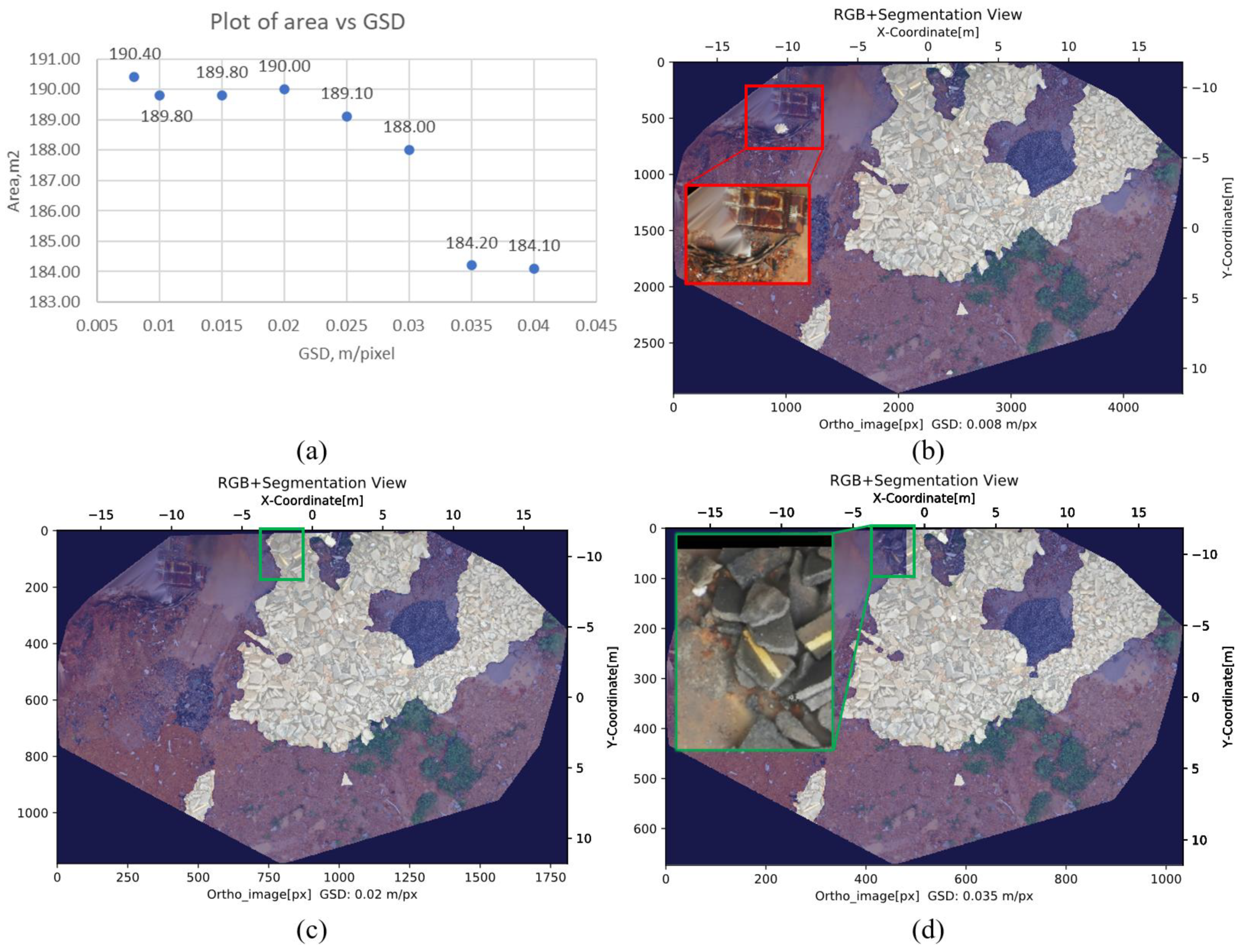
The extracted WC stockpiles are shown in Figure 11d–f and have the projected areas summarized in Figure 13a. The U-Net-generated label images for GSD = 0.008, 0.02, and 0.035 m/pixel are shown in Figure 13b–d, respectively, with the annotated difference and the detailed section, as well. Among the different GSDs, only the GSD = 0.035 and 0.04 m/pixel have significantly different area values compared to others. Figure 13c,d explains that the marked section containing concrete debris is much darker than the others and close to the aggregate particles, resulting in the U-Net failing to identify them as WC objects.
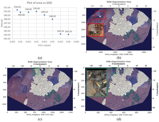
Figure 13.
Feature image GSD sensitivity analysis: (a) plot of area vs GSD, (b) GSD = 0.008 m/pixel, (c) GSD = 0.020 m/pixel, and (d) GSD = 0.035 m/pixel.
Furthermore, Figure 11 indicates that the P2O orthoimages filled gaps on their edges with similar textures from neighboring pixels, especially in the annotated top-left corners of Figure 11a,d. When GSD = 0.008, 0.010, and 0.015 m/pixel, the U-Net model incorrectly identified a piece of WC debris in the filled regions, as shown in Figure 13b, but this error did not occur in other GSDs. The filled regions in the P2O feature image can be removed by comparing them with the original point cloud. Therefore, the proposed DA can enable the FCN to perform accurate pixelwise segmentation on P2O orthoimages with GSD = 0.008 to 0.03 m/pixel (0.86 to 3.24 times of 0.009261 m/pixel), which enhanced the designed the GSD range of 2/3 to 2 times of the training data sets.
5.2. Screenshot Feature Image and Point Cloud Display Size Parameter Analysis in Measurement Performance
The results in Figure 11a,d show that the extracted WC stockpiles for the screenshot feature images and P2O feature images have a 1.15% area difference and a 5% volume difference. Based on Equation (3b), the average heights of the WC stockpiles are different between the two sets of feature images, as well. The elevation values for the P2O feature images are directly obtained from the original point cloud, which are the ground truth values. The measured WC stockpiles’ average height is 0.523 m for GSD = 0.020, 0.025, and 0.030 m/pixel. It is 3.86% = (100 − 0.523/0.544 × 100)% or 0.021 m less than the screenshot feature images with an average height of 0.544 m. According to Equation (2), the elevations of screenshot feature images are converted from the 8-bit grayscale images. As shown in Figure 10a, by setting = −1 m and = 4 m, the interval of adjacent integers between 0 and 255 represents an elevation change of 0.0196 m, which means the elevation values have a precision of ±0.0196 m. Thus, a majority (93.33%) of elevation differences result from the grayscale elevation images, and we further investigated whether or not the point size would result in the additional 6.67% (0.0014 m) elevation difference.
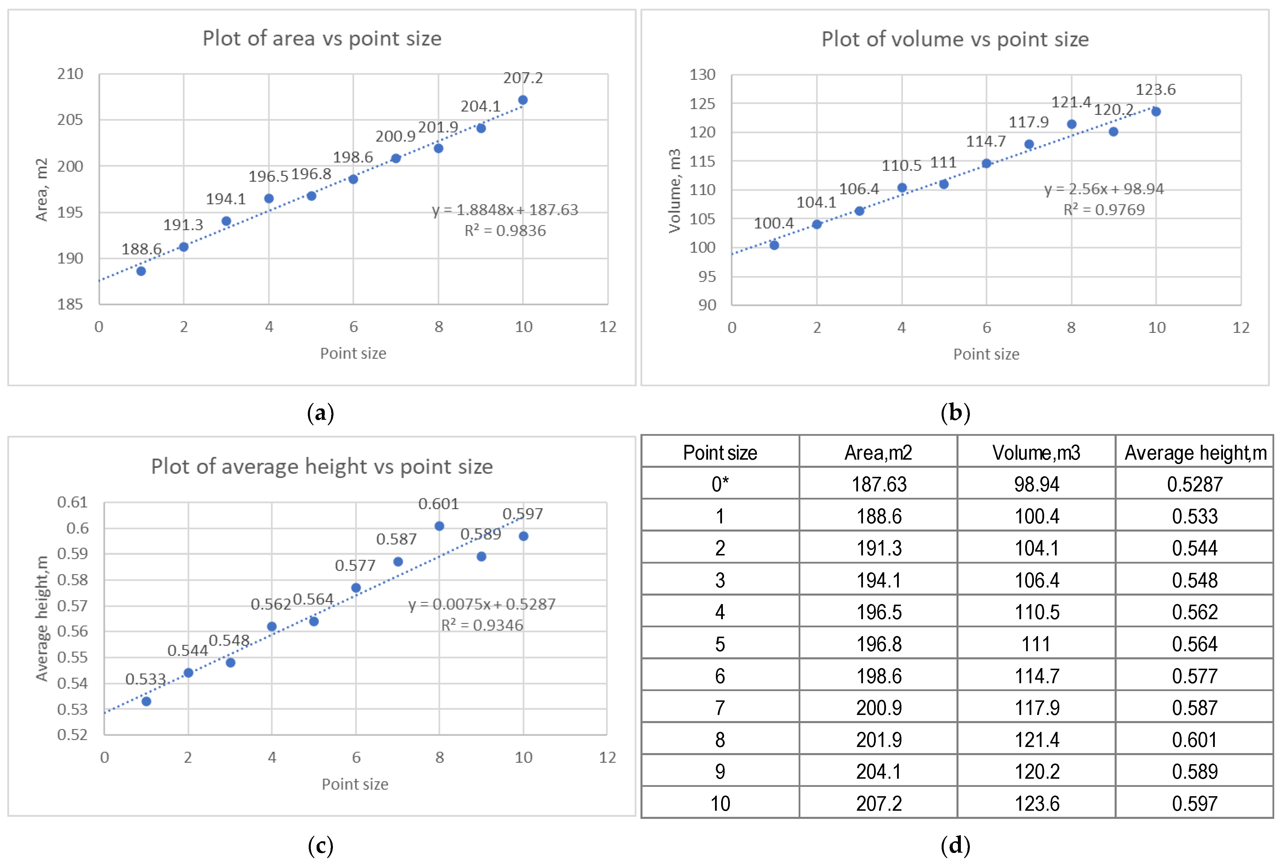
The ReCap Pro software has a default point cloud display size of 2, and supports display sizes in the range of 1 to 10. The sensitivity analysis of point cloud display size was conducted, and the results are shown in Figure 14, where the area, average height, and volume of the extracted WC stockpiles have a positive relationship and are sensitive to point sizes in the range of 1 to 10. Reasons were investigated and analyzed as follows: (1) when the point size is small, the scattered thin WC pieces were dropped by the 10,000-pixel area filter, e.g., the annotated WC pieces in Figure 11a,b; (2) when the point size is large, e.g., point size of 10 in Figure 11c, the gaps in the RGB image and elevation image were filled, but this also resulted in WC points invading non-WC regions when compared to smaller point size values, e.g., point size of 1 shown in Figure 11b. As a result, the U-Net-generated pixelwise label image detected more WC pixels and resulted in the projected area of the extracted WC stockpile increasing by 18.6 m2 (or 9.86%) when comparing point sizes 1 and 10.
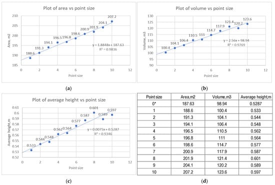
Figure 14.
Point cloud display size sensitivity analysis: (a) plot of area vs point size, (b) plot of volume vs point size, (c) plot of average height vs point size, and (d) detailed results (* indicates the predictions).
Additionally, the average height of the WC stockpile has a difference of 0.064 m (or 12.01%) between point sizes 10 and 1. As a result, the estimated volume of the WC stockpile has a difference of 23.2 m3 (or 23.11%). After eliminating the impact of point size by setting the point size as zero, the estimated area, volume, and average height from the linear regressions are 187.63 m2, 98.94 m3, and 0.5287 m, which are close to the results of 189.10 m2, 98.90 m3, and 0.523 m from the P2O feature image with GSD = 0.025 m/pixel. Therefore, in future applications, when using the developed screenshot tool with ReCap Pro, setting the point cloud display size at the default value of 2 in ReCap Pro is recommended for C&D debris object detection when the collected point clouds are sufficiently dense; otherwise, the Pointcloud2Orthoimage tool is recommended for C&D debris object measurement.
5.3. Benefits for Construction Waste Management Practice
As shown in Figure 1, most C&D debris illegal dumping sites contain hazards for in-person investigation. Using a drone and photogrammetry to obtain the 3D reality data of the C&D debris stockpiles is a convenient and safe approach for field investigation. The field investigator can first fly a drone at a higher altitude to have the overall view of an illegal dumping site, then fly the drone at a lower altitude to capture the detailed images (both top and side views) for SfM photogrammetry to generate 3D point clouds for the illegal dumping site. Following that, the developed method can provide quantitative analyses of occupied land area and debris volume in order to penalize the illegal dumping of C&D debris. In detail, the deep learning-based image segmentation method allows automated detection of C&D debris and the projected area measurement; the point cloud-generated elevation data make volume calculation feasible for the C&D debris stockpiles detected from the point cloud-generated RGB orthoimage.
Since construction wastes’ quantities are known, moving and cleaning tasks are easy to plan and optimize, such as determining equipment cycle time and production rate, and deciding the optimal number of trucks. Moreover, if the city government has proposed penalties for illegal dumping of C&D waste with unit penalty prices, then this quantitative information can be used for calculating the total fines for illegal dumping of C&D waste and will help the government to investigate the party responsible for the illegal dumping of C&D waste and more fairly impose penalties on illegal dumping activity. Additionally, at construction sites or demolition jobsites, different categories of C&D materials can be accurately detected from a single point cloud-generated RGB orthoimage via a single FCN or separate specialized FCNs; the hazardous waste and recycled C&D materials can then be further classified. As a result, through improved categorization, reasonable C&D waste treatment plans can be proposed for different C&D materials, such as backfilling muck at other construction sites and recycling concrete debris as coarse and fine aggregates.
Furthermore, the developed method in this study provides geographic information relating to C&D debris stockpiles to support the government’s C&D waste intelligent monitoring and information management. Using drones, LiDAR, and deep learning technologies can allow investigators to automatically obtain the volume data and as-built models of C&D waste generated at construction sites or demolition jobsites, and the stockpiled C&D waste at landfill sites or illegal dumping sites. By importing and maintaining the quantitative information in the construction waste intelligent information management system, the city government and related departments can assess the stacking, transportation, and treatment status of C&D waste within its jurisdiction in real-time [51,52]. Moreover, the enhanced construction waste intelligent information management system (Figure 2) can provide useful information for C&D material recycling firms in lean production since the C&D debris inventory is accessible from the information system, overcome barriers to reverse logistics in C&D waste [53], as well as reduce the transportation costs by using C&D wastes’ GIS information for route optimization.
5.4. Limitations and Recommendations
This research did not evaluate the accuracy of the photogrammetry results and assumed they are correct. Previous studies indicated that the measurement performance of photogrammetry with camera drones has a 5 cm error in both horizontal and vertical coordinates [16,31,32]. Future research could lay out several ground control points and check points to enhance the accuracy of photogrammetry. For example, a drone landing pad of known size (e.g., 75 cm) can be placed next to the C&D debris; then, the landing pad will be present in the point cloud-generated orthoimage and can be detected via an additional FCN model. As a result, the actual GSD of the feature images can then be determined via the ratio of the landing pad diameter in meters to the landing pad diameter in pixel units. Furthermore, we did not evaluate the accuracy of the results of automatic volume calculations against other traditional surveying methods such as total stations and GPS devices. Future research is recommended in such comparisons to determine the accuracy of drone-based photogrammetry volume calculations.
Additionally, the developed method can process both photogrammetric point clouds and laser scanning point clouds automatically. For example, mobile devices, i.e., iPad Pro and iPhone Pro with LiDAR sensors, could be used to quickly scan C&D debris stockpiles. Then, the developed P2O tool can automatically convert a 3D point cloud file to a 2D feature image of orthoimage and elevation data files, such as the examples in [45]. Any preferred GSD value, e.g., 0.010 m/pixel, can then be used to generate the feature images. As the image frame is not limited by a screenshot, any scanned large-sized C&D landfill and dumping site can be presented in a high-resolution image. In addition, the step of converting the elevation range to the grayscale value range [0, 255] can be skipped because the elevation information can be directly accessed at each point. Bypassing this step also eliminates the possible loss of elevation data precision that might occur in this step.
Furthermore, the designed conventional encoder-decoder can be trained with label images that contain multiple categories of C&D materials; the pixelwise segmentation results generated by the conventional encoder-decoder will then assign the corresponding labels to the different C&D debris stockpiles, like the example in [45]. The U-Net can also be applied to detect multiple categories of C&D materials, with two potential approaches: (1) training separate U-Nets for different C&D material detections, as U-Net has the advantage of requiring fewer training data samples to develop a well-trained model; and (2) modifying U-Net to support multiple object detection by replacing the Sigmoid activation function with the SoftMax activation function in the end layer. However, for the latter option, label image one-hot encoding is required, and then a powerful workstation with more memory is required for loading the one-hot labels. Thus, future applications should prepare the training data sets and select the FCN models depending on the task’s requirements.
6. Conclusions
The purpose of this research was to develop a time- and cost-efficient method for construction waste management at construction and demolition jobsites, landfill sites, and illegal dumping sites, using drones and camera-based C&D debris scanning, SfM photogrammetry-based C&D debris 3D reconstruction, FCN image segmentation-based C&D debris extraction and measurement, as well as ArcGIS-based C&D debris information management with as-built 2D CAD drawings and 3D point clouds (see Figure 3). The main findings of the experiments and parameter analysis are summarized as follows:
(1) Scanning C&D stockpiles with a low-cost, ready-to-fly consumer drone, e.g., DJI Mavic 2 Pro (USD 1599), to obtain C&D debris stockpiles’ top-view and side-view images can be effectively used with the SfM photogrammetry approach to generate dense 3D point clouds for C&D debris area.
(2) Using the Pointcloud2Orthoimage tool can convert 3D point clouds into 2D feature images of RGB orthoimage and elevation data for automatic, robust, and accurate C&D debris object measurement. Both the light convolutional encoder-decoder network (Table 2) and the U-Net can be effectively trained for C&D debris detection with relatively few data sets of images and label images through the data augmentation strategies. In this study, the U-Net performed better, with a concrete debris IoU value of 0.9006 in testing data sets (see Table 3).
The method developed in this study provides quantitative and geographic information to support city governments and the related departments in C&D debris intelligent information management (see Figure 2).
Author Contributions
Conceptualization, Y.J. and J.L.; methodology, Y.J.; software, Y.J. and D.L.; validation, Y.J. and Y.H.; investigation, Y.J. and S.L.; data collection, W.N. and I.-H.C.; writing—original draft preparation, Y.J.; writing—review and editing, Y.J., Y.H. and J.L. All authors have read and agreed to the published version of the manuscript.
Funding
This research received no external funding.
Data Availability Statement
The training and testing data sets and the Python codes are available in [45].
Acknowledgments
The authors are grateful to the reviewers for their valuable suggestions.
Conflicts of Interest
The authors declare no conflict of interest.
References
- CEMBUREAU Activity Report. 2020. Available online: https://www.cembureau.eu/media/m2ugw54y/cembureau-2020-activity-report.pdf (accessed on 18 July 2021).
- CEMBUREAU Activity Report. 2019. Available online: https://cembureau.eu/media/clkdda45/activity-report-2019.pdf (accessed on 19 July 2021).
- Mohammed, T.U.; Hasnat, A.; Awal, M.A.; Bosunia, S.Z. Recycling of Brick Aggregate Concrete as Coarse Aggregate. J. Mater. Civ. Eng. 2015, 27, B4014005. [Google Scholar] [CrossRef]
- De Brito, J.; Silva, R. Current Status on the Use of Recycled Aggregates in Concrete: Where Do We Go from Here? RILEM Tech. Lett. 2016, 1, 1–5. [Google Scholar] [CrossRef]
- Eurostat Waste Statistics. Available online: https://ec.europa.eu/eurostat/statistics-explained/index.php?title=Waste_statistics#Total_waste_generation (accessed on 18 July 2021).
- Wu, B.; Yu, Y.; Chen, Z.; Zhao, X. Shape Effect on Compressive Mechanical Properties of Compound Concrete Containing Demolished Concrete Lumps. Constr. Build. Mater. 2018, 187, 50–64. [Google Scholar] [CrossRef]
- Zhao, W.; Rotter, S. The Current Situation of Construction & Demolition Waste Management in China. In Proceedings of the 2008 2nd International Conference on Bioinformatics and Biomedical Engineering, Shanghai, China, 16–18 May 2008; pp. 4747–4750. [Google Scholar]
- Zheng, L.; Wu, H.; Zhang, H.; Duan, H.; Wang, J.; Jiang, W.; Dong, B.; Liu, G.; Zuo, J.; Song, Q. Characterizing the Generation and Flows of Construction and Demolition Waste in China. Constr. Build. Mater. 2017, 136, 405–413. [Google Scholar] [CrossRef]
- Islam, R.; Nazifa, T.H.; Yuniarto, A.; Shanawaz Uddin, A.S.M.; Salmiati, S.; Shahid, S. An Empirical Study of Construction and Demolition Waste Generation and Implication of Recycling. Waste Manag. 2019, 95, 10–21. [Google Scholar] [CrossRef]
- U.S. Environmental Protection Agency Sustainable Management of Construction and Demolition Materials. Available online: https://www.epa.gov/smm/sustainable-management-construction-and-demolition-materials (accessed on 19 July 2021).
- Shenzhen Housing and Construction Bureau Shenzhen Construction Waste Management Methods. Available online: http://www.sz.gov.cn/cn/xxgk/zfxxgj/zcfg/szsfg/content/post_8201973.html (accessed on 9 April 2022).
- Biotto, G.; Silvestri, S.; Gobbo, L.; Furlan, E.; Valenti, S.; Rosselli, R. GIS, Multi-criteria and Multi-factor Spatial Analysis for the Probability Assessment of the Existence of Illegal Landfills. Int. J. Geogr. Inf. Sci. 2009, 23, 1233–1244. [Google Scholar] [CrossRef]
- Silvestri, S.; Omri, M. A Method for the Remote Sensing Identification of Uncontrolled Landfills: Formulation and Validation. Int. J. Remote Sens. 2008, 29, 975–989. [Google Scholar] [CrossRef]
- Yan, W.Y.; Mahendrarajah, P.; Shaker, A.; Faisal, K.; Luong, R.; Al-Ahmad, M. Analysis of Multi-Temporal Landsat Satellite Images for Monitoring Land Surface Temperature of Municipal Solid Waste Disposal Sites. Environ. Monit. Assess. 2014, 186, 8161–8173. [Google Scholar] [CrossRef]
- Ashtiani, M.Z.; Muench, S.T.; Gent, D.; Uhlmeyer, J.S. Application of Satellite Imagery in Estimating Stockpiled Reclaimed Asphalt Pavement (RAP) Inventory: A Washington State Case Study. Constr. Build. Mater. 2019, 217, 292–300. [Google Scholar] [CrossRef]
- Jiang, Y.; Bai, Y. Low–High Orthoimage Pairs-Based 3D Reconstruction for Elevation Determination Using Drone. J. Constr. Eng. Manag. 2021, 147, 04021097. [Google Scholar] [CrossRef]
- Park, J.W.; Yeom, D.J. Method for Establishing Ground Control Points to Realize UAV-Based Precision Digital Maps of Earthwork Sites. J. Asian Archit. Build. Eng. 2021, 21, 110–119. [Google Scholar] [CrossRef]
- Kavaliauskas, P.; Židanavičius, D.; Jurelionis, A. Geometric Accuracy of 3D Reality Mesh Utilization for BIM-Based Earthwork Quantity Estimation Workflows. ISPRS Int. J. Geo-Inf. 2021, 10, 399. [Google Scholar] [CrossRef]
- Elkhrachy, I. Accuracy Assessment of Low-Cost Unmanned Aerial Vehicle (UAV) Photogrammetry. Alex. Eng. J. 2021, 60, 5579–5590. [Google Scholar] [CrossRef]
- Jiang, Y.; Bai, Y. Determination of Construction Site Elevations Using Drone Technology. In Proceedings of the Construction Research Congress 2020, Tempe, Arizona, 8–10 March 2020; American Society of Civil Engineers: Reston, VA, USA, 2020; pp. 296–305. [Google Scholar]
- Han, S.; Jiang, Y. Construction Site Top-View Generation Using Drone Imagery: The Automatic Stitching Algorithm Design and Application. In Proceedings of the The 12th International Conference on Construction in the 21st Century (CITC-12), Amman, Jordan, 16–19 May 2022; pp. 326–334. [Google Scholar]
- Jiang, Y.; Han, S.; Bai, Y. Building and Infrastructure Defect Detection and Visualization Using Drone and Deep Learning Technologies. J. Perform. Constr. Facil. 2021, 35, 04021092. [Google Scholar] [CrossRef]
- Seo, J.; Duque, L.; Wacker, J. Drone-Enabled Bridge Inspection Methodology and Application. Autom. Constr. 2018, 94, 112–126. [Google Scholar] [CrossRef]
- Chen, K.; Reichard, G.; Akanmu, A.; Xu, X. Geo-Registering UAV-Captured Close-Range Images to GIS-Based Spatial Model for Building Façade Inspections. Autom. Constr. 2021, 122, 103503. [Google Scholar] [CrossRef]
- Chen, K.; Reichard, G.; Xu, X.; Akanmu, A. Automated Crack Segmentation in Close-Range Building Façade Inspection Images Using Deep Learning Techniques. J. Build. Eng. 2021, 43, 102913. [Google Scholar] [CrossRef]
- Yeh, C.C.; Chang, Y.L.; Alkhaleefah, M.; Hsu, P.H.; Eng, W.; Koo, V.C.; Huang, B.; Chang, L. YOLOv3-Based Matching Approach for Roof Region Detection from Drone Images. Remote Sens. 2021, 13, 127. [Google Scholar] [CrossRef]
- Jiang, Y.; Han, S.; Bai, Y. Scan4Façade: Automated As-Is Façade Modeling of Historic High-Rise Buildings Using Drones and AI. J. Archit. Eng. 2022, 28, 04022031. [Google Scholar] [CrossRef]
- Mishra, B.; Garg, D.; Narang, P.; Mishra, V. Drone-Surveillance for Search and Rescue in Natural Disaster. Comput. Commun. 2020, 156, 1–10. [Google Scholar] [CrossRef]
- Kyrkou, C.; Theocharides, T. EmergencyNet: Efficient Aerial Image Classification for Drone-Based Emergency Monitoring Using Atrous Convolutional Feature Fusion. IEEE J. Sel. Top. Appl. Earth Obs. Remote Sens. 2020, 13, 1687–1699. [Google Scholar] [CrossRef]
- Kyrkou, C.; Theocharides, T. Deep-Learning-Based Aerial Image Classification for Emergency Response Applications Using Unmanned Aerial Vehicles. In Proceedings of the 2019 IEEE/CVF Conference on Computer Vision and Pattern Recognition Workshops (CVPRW), Long Beach, CA, USA, 16–17 June 2019; pp. 517–525. [Google Scholar]
- Takahashi, N.; Wakutsu, R.; Kato, T.; Wakaizumi, T.; Ooishi, T.; Matsuoka, R. Experiment on UAV Photogrammetry and Terrestrial Laser Scanning for ICT-Integrated Construction. ISPRS—Int. Arch. Photogramm. Remote Sens. Spat. Inf. Sci. 2017, XLII-2/W6, 371–377. [Google Scholar] [CrossRef]
- Han, S.; Jiang, Y.; Bai, Y. Fast-PGMED: Fast and Dense Elevation Determination for Earthwork Using Drone and Deep Learning. J. Constr. Eng. Manag. 2022, 148, 04022008. [Google Scholar] [CrossRef]
- Haur, C.J.; Kuo, L.S.; Fu, C.P.; Hsu, Y.L.; Heng, C. Da Feasibility Study on UAV-Assisted Construction Surplus Soil Tracking Control and Management Technique. IOP Conf. Ser. Mater. Sci. Eng. 2018, 301, 012145. [Google Scholar] [CrossRef]
- Zhang, Q.; Zhang, X.; Mu, X.; Wang, Z.; Tian, R.; Wang, X.; Liu, X. Recyclable Waste Image Recognition Based on Deep Learning. Resour. Conserv. Recycl. 2021, 171, 105636. [Google Scholar] [CrossRef]
- Davis, P.; Aziz, F.; Newaz, M.T.; Sher, W.; Simon, L. The Classification of Construction Waste Material Using a Deep Convolutional Neural Network. Autom. Constr. 2021, 122, 103481. [Google Scholar] [CrossRef]
- Chen, J.; Lu, W.; Xue, F. “Looking beneath the Surface”: A Visual-Physical Feature Hybrid Approach for Unattended Gauging of Construction Waste Composition. J. Environ. Manag. 2021, 286, 112233. [Google Scholar] [CrossRef]
- Wang, Z.; Li, H.; Zhang, X. Construction Waste Recycling Robot for Nails and Screws: Computer Vision Technology and Neural Network Approach. Autom. Constr. 2019, 97, 220–228. [Google Scholar] [CrossRef]
- Zhang, S.; Chen, Y.; Yang, Z.; Gong, H. Computer Vision Based Two-Stage Waste Recognition-Retrieval Algorithm for Waste Classification. Resour. Conserv. Recycl. 2021, 169, 105543. [Google Scholar] [CrossRef]
- Jiang, Y.; Han, S.; Bai, Y. Development of a Pavement Evaluation Tool Using Aerial Imagery and Deep Learning. J. Transp. Eng. Part B Pavements 2021, 147, 04021027. [Google Scholar] [CrossRef]
- Jiang, Y.; Bai, Y.; Han, S. Determining Ground Elevations Covered by Vegetation on Construction Sites Using Drone-Based Orthoimage and Convolutional Neural Network. J. Comput. Civ. Eng. 2020, 34, 04020049. [Google Scholar] [CrossRef]
- Jiang, Y. Remote Sensing and Neural Network-Driven Pavement Evaluation: A Review. In Proceedings of the 12th International Conference on Construction in the 21st Century (CITC-12), Amman, Jordan, 16–19 May 2022; pp. 335–345. [Google Scholar]
- Jiang, Y.; Han, S.; Li, D.; Bai, Y.; Wang, M. Automatic Concrete Sidewalk Deficiency Detection and Mapping with Deep Learning. Expert Syst. Appl. 2022, 207, 117980. [Google Scholar] [CrossRef]
- Autodesk 3D View. Available online: https://help.autodesk.com/view/RECAP/ENU/?guid=Reality_Capture_View_and_Navigate_Point_Cloud_Color_Settings_3D_View_html (accessed on 22 June 2021).
- OpenCV Smoothing Images. Available online: https://docs.opencv.org/3.4/dc/dd3/tutorial_gausian_median_blur_bilateral_filter.html (accessed on 22 June 2021).
- Jiang, Y. Demo of Concrete Debris Measurement and Mapping. Available online: https://www.yuhanjiang.com/research/UCPD/CDWM/CD (accessed on 27 August 2022).
- Ronneberger, O.; Fischer, P.; Brox, T. U-Net: Convolutional Networks for Biomedical Image Segmentation. In Lecture Notes in Computer Science (Including Subseries Lecture Notes in Artificial Intelligence and Lecture Notes in Bioinformatics); Springer: Cham, Switzerland, 2015; Volume 9351, pp. 234–241. ISBN 9783319245737. [Google Scholar]
- Zhi, X. Implementation of Deep Learning Framework—Unet, Using Keras. Available online: https://github.com/zhixuhao/unet (accessed on 1 July 2020).
- Jiang, Y.; Han, S.; Bai, Y. Construction Site Segmentation Using Drone-Based Ortho-Image and Convolutional Encoder-Decoder Network Model. In Proceedings of the Construction Research Congress 2022, Arlington, VA, USA, 7–12 March 2022; American Society of Civil Engineers: Reston, VA, USA, 2022; pp. 1096–1105. [Google Scholar]
- Haeberli, P.; Voorhies, D. Image Processing by Interp and Extrapolation. Available online: http://www.graficaobscura.com/interp/index.html (accessed on 28 July 2021).
- OpenCV Contours in OpenCV. Available online: https://docs.opencv.org/3.4/d3/d05/tutorial_py_table_of_contents_contours.html (accessed on 9 November 2020).
- Zainun, N.Y.; Rahman, I.A.; Rothman, R.A. Mapping Of Construction Waste Illegal Dumping Using Geographical Information System (GIS). IOP Conf. Ser. Mater. Sci. Eng. 2016, 160, 012049. [Google Scholar] [CrossRef]
- Wu, H.; Wang, J.; Duan, H.; Ouyang, L.; Huang, W.; Zuo, J. An Innovative Approach to Managing Demolition Waste via GIS (Geographic Information System): A Case Study in Shenzhen City, China. J. Clean. Prod. 2016, 112, 494–503. [Google Scholar] [CrossRef]
- Correia, J.M.F.; de Oliveira Neto, G.C.; Leite, R.R.; da Silva, D. Plan to Overcome Barriers to Reverse Logistics in Construction and Demolition Waste: Survey of the Construction Industry. J. Constr. Eng. Manag. 2021, 147, 04020172. [Google Scholar] [CrossRef]

Publisher’s Note: MDPI stays neutral with regard to jurisdictional claims in published maps and institutional affiliations. |
© 2022 by the authors. Licensee MDPI, Basel, Switzerland. This article is an open access article distributed under the terms and conditions of the Creative Commons Attribution (CC BY) license (https://creativecommons.org/licenses/by/4.0/).