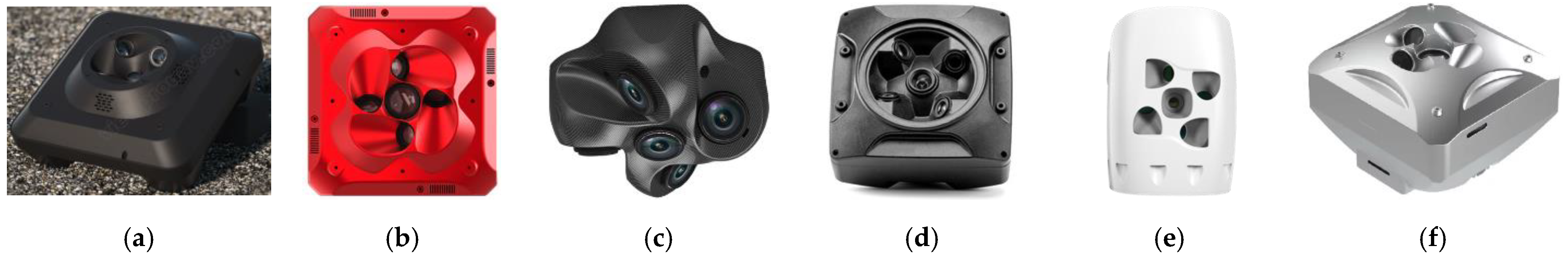
Figure 1.
Example of commercially available multi-view cameras for UAV platform (
Table 1): Viewprouav (
a), Shareuavtex (
b), DroneBase (
c), ADTi (
d), Quantum-System (
e), and JOUAV (
f).
Figure 1.
Example of commercially available multi-view cameras for UAV platform (
Table 1): Viewprouav (
a), Shareuavtex (
b), DroneBase (
c), ADTi (
d), Quantum-System (
e), and JOUAV (
f).
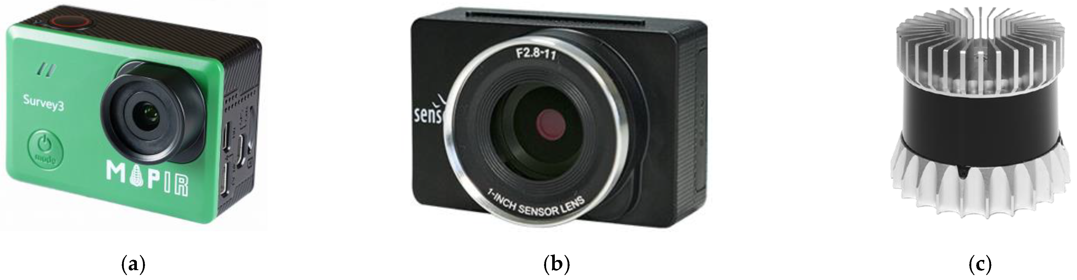
Figure 2.
The chosen MAPIR Survey 3 (a), senseFly SODA (b), and Ouster OS1-32 (c).
Figure 2.
The chosen MAPIR Survey 3 (a), senseFly SODA (b), and Ouster OS1-32 (c).
Figure 3.
Hybrid MAPIR + Ouster system showing its internal arrangement, dimensions, and footprint patterns on the ground (a); hybrid senseFly + Ouster system showing its internal arrangement, dimensions, and footprint patterns on the ground (b).
Figure 3.
Hybrid MAPIR + Ouster system showing its internal arrangement, dimensions, and footprint patterns on the ground (a); hybrid senseFly + Ouster system showing its internal arrangement, dimensions, and footprint patterns on the ground (b).
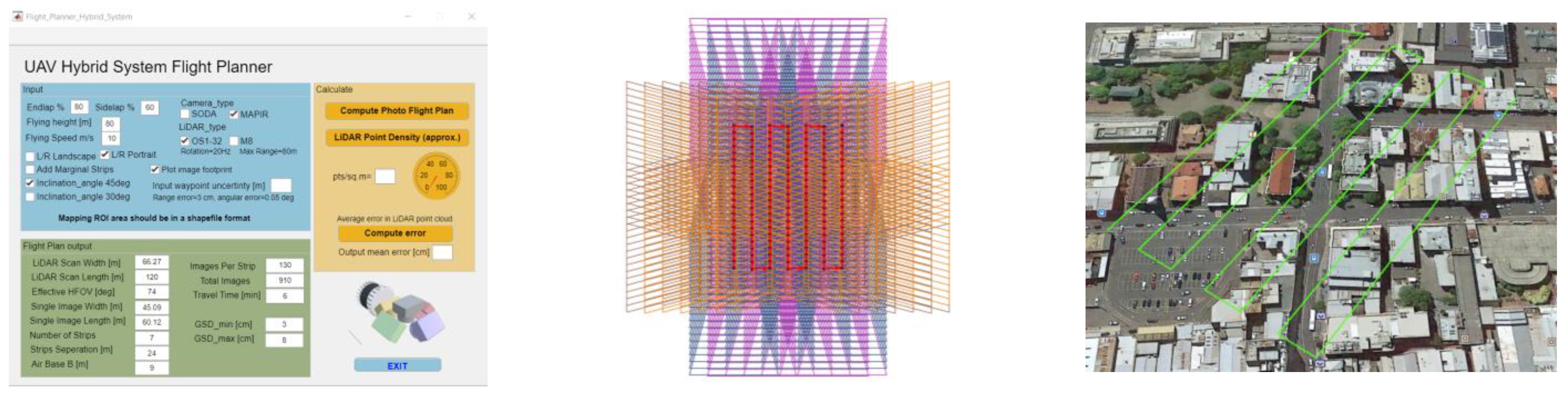
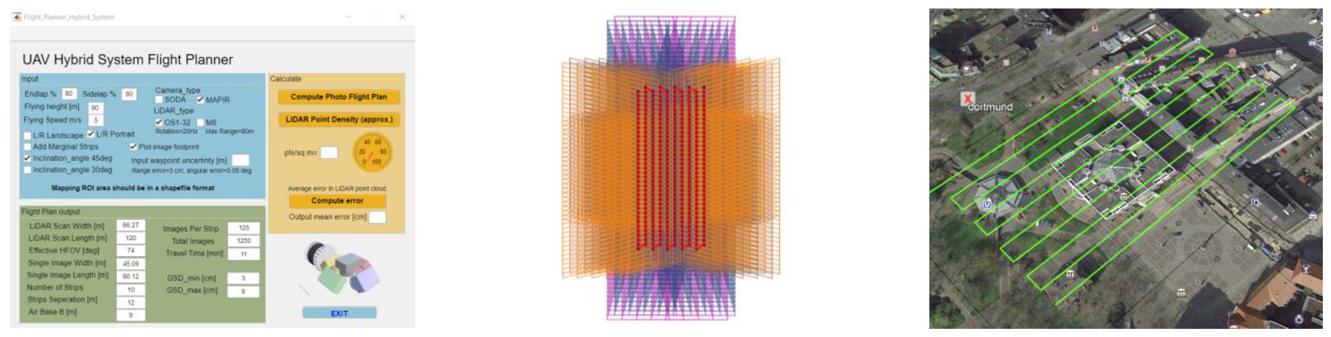
Figure 4.
The GUI of the developed flight planning tool for hybrid UAV-based sensors (a). The image footprints plot for a given flight and sensor configuration (b).
Figure 4.
The GUI of the developed flight planning tool for hybrid UAV-based sensors (a). The image footprints plot for a given flight and sensor configuration (b).
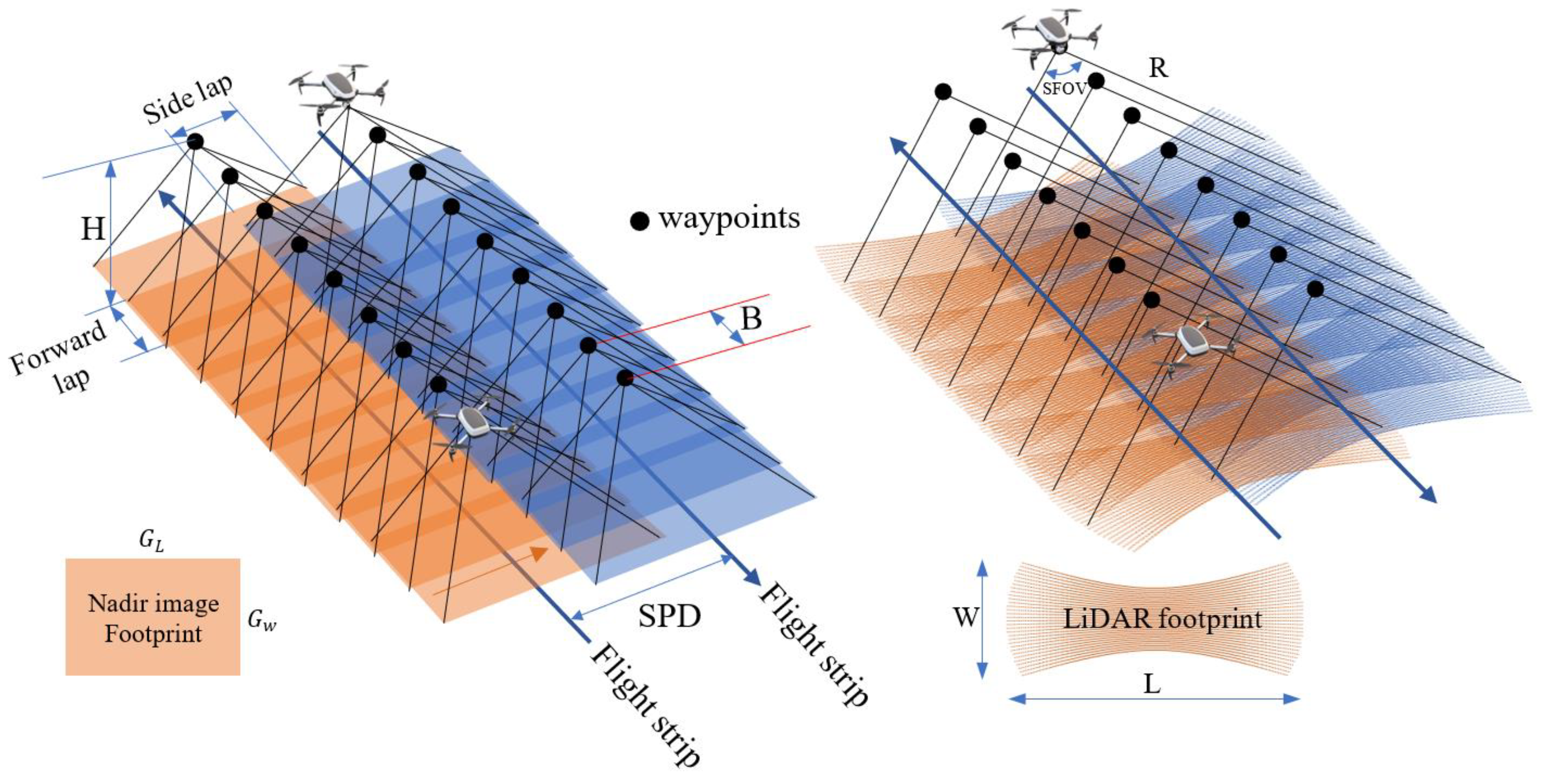
Figure 5.
UAV flight planning design parameters illustration for both sensors used.
Figure 5.
UAV flight planning design parameters illustration for both sensors used.
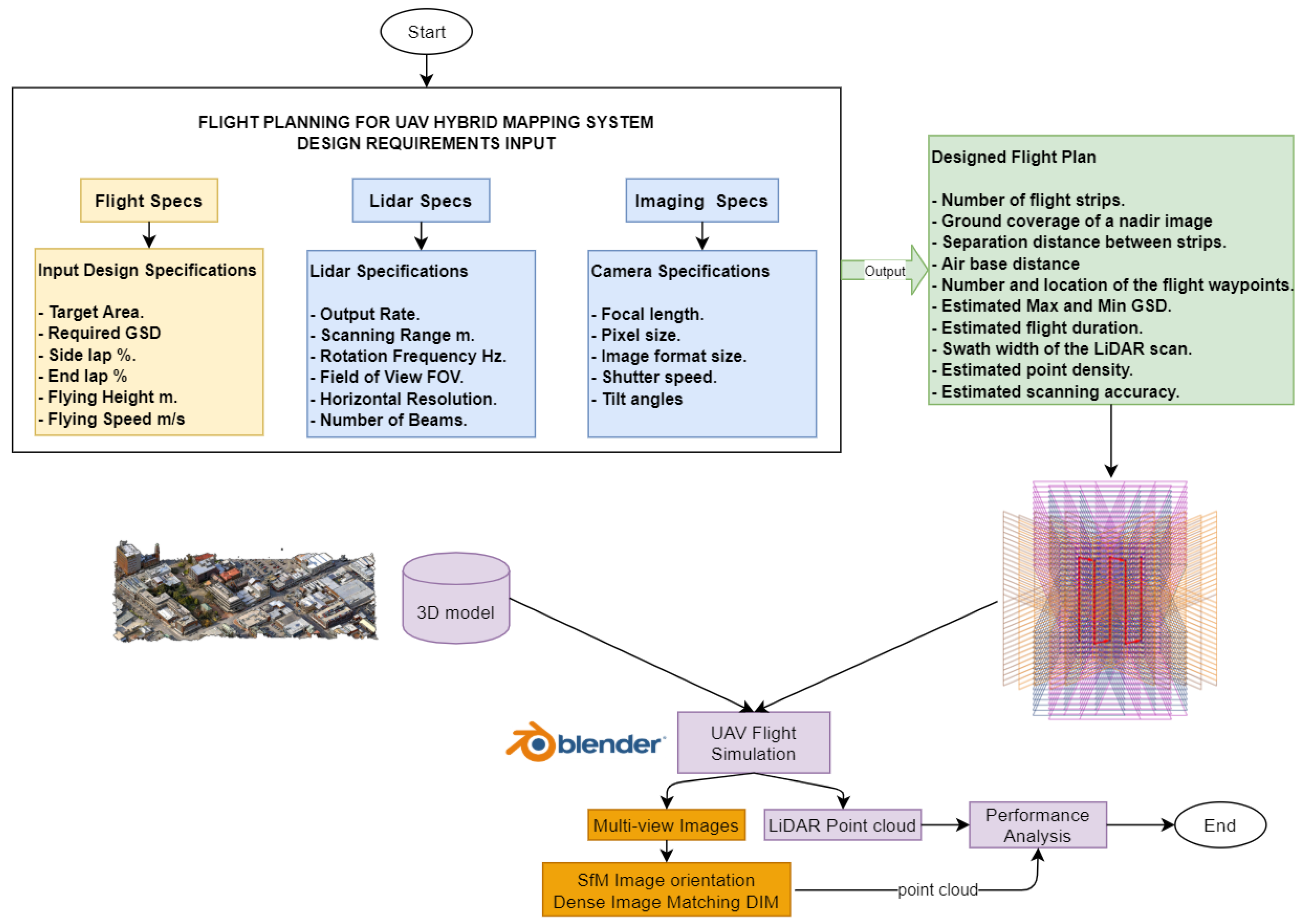
Figure 6.
Methodology workflow.
Figure 6.
Methodology workflow.
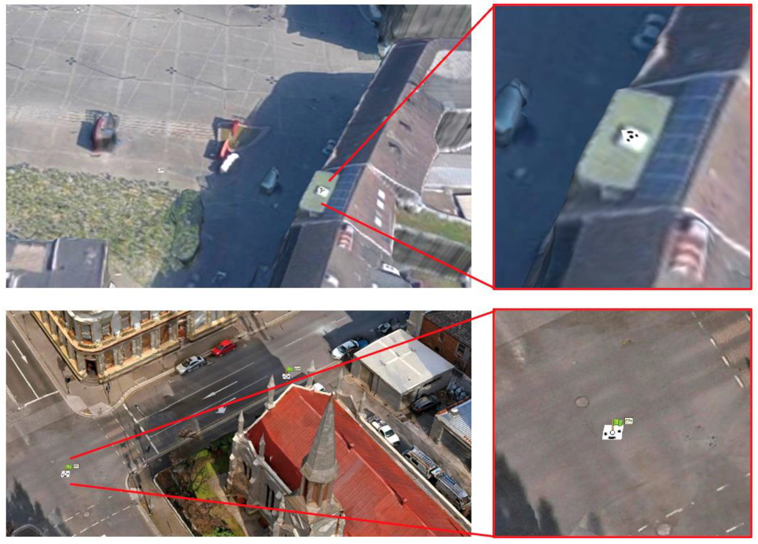
Figure 7.
Examples of the GCPs/CPs used in the photogrammetric adjustments of the simulated datasets.
Figure 7.
Examples of the GCPs/CPs used in the photogrammetric adjustments of the simulated datasets.
Figure 8.
Flight planning with the senseFly camera over Launceston: five strips and 475 multi-view images.
Figure 8.
Flight planning with the senseFly camera over Launceston: five strips and 475 multi-view images.
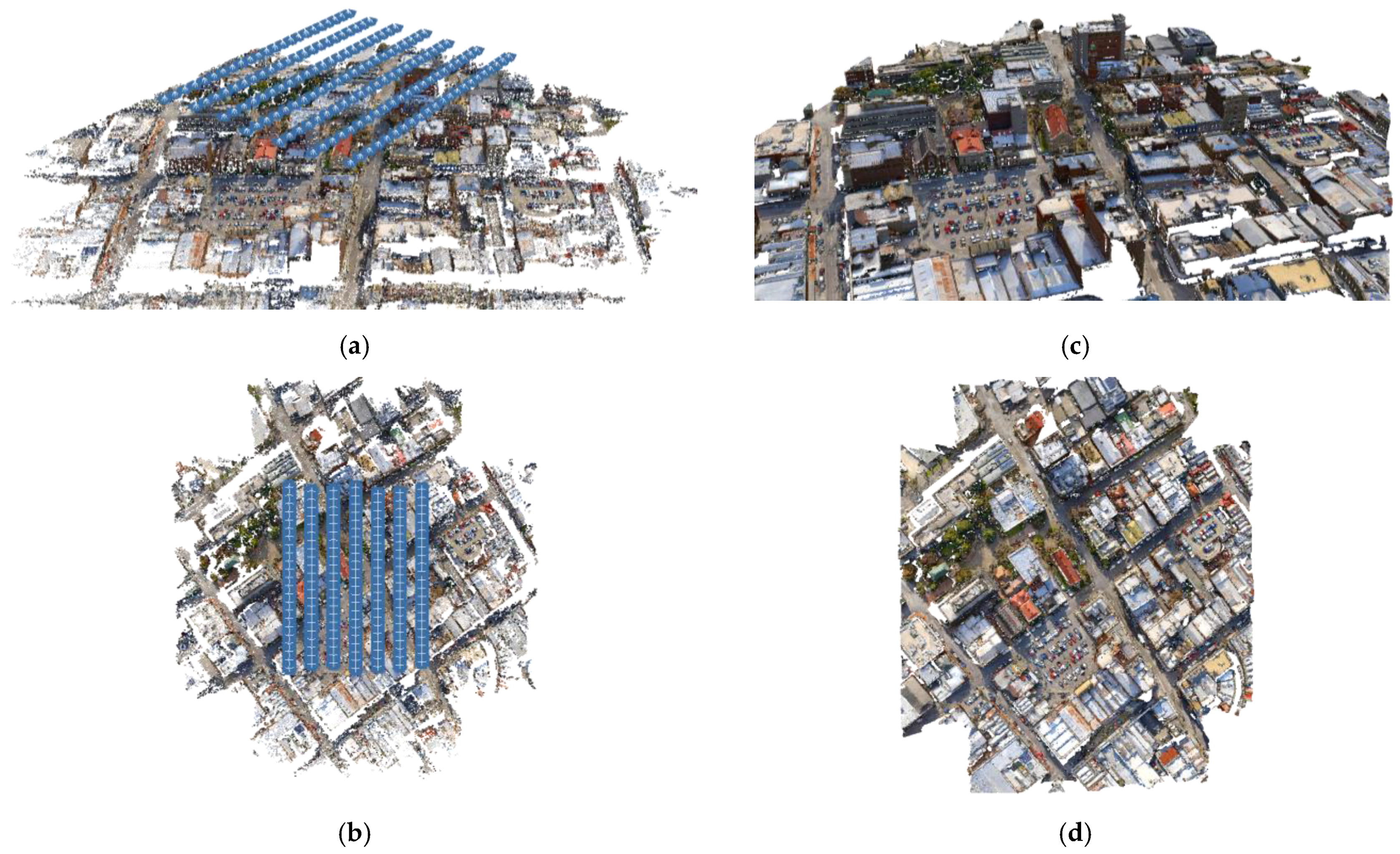
Figure 9.
Recovered camera poses and sparse point cloud for the simulated senseFly-based multi-view image block (475 images) over Launceston (a,b). Derived dense point cloud (c,d).
Figure 9.
Recovered camera poses and sparse point cloud for the simulated senseFly-based multi-view image block (475 images) over Launceston (a,b). Derived dense point cloud (c,d).
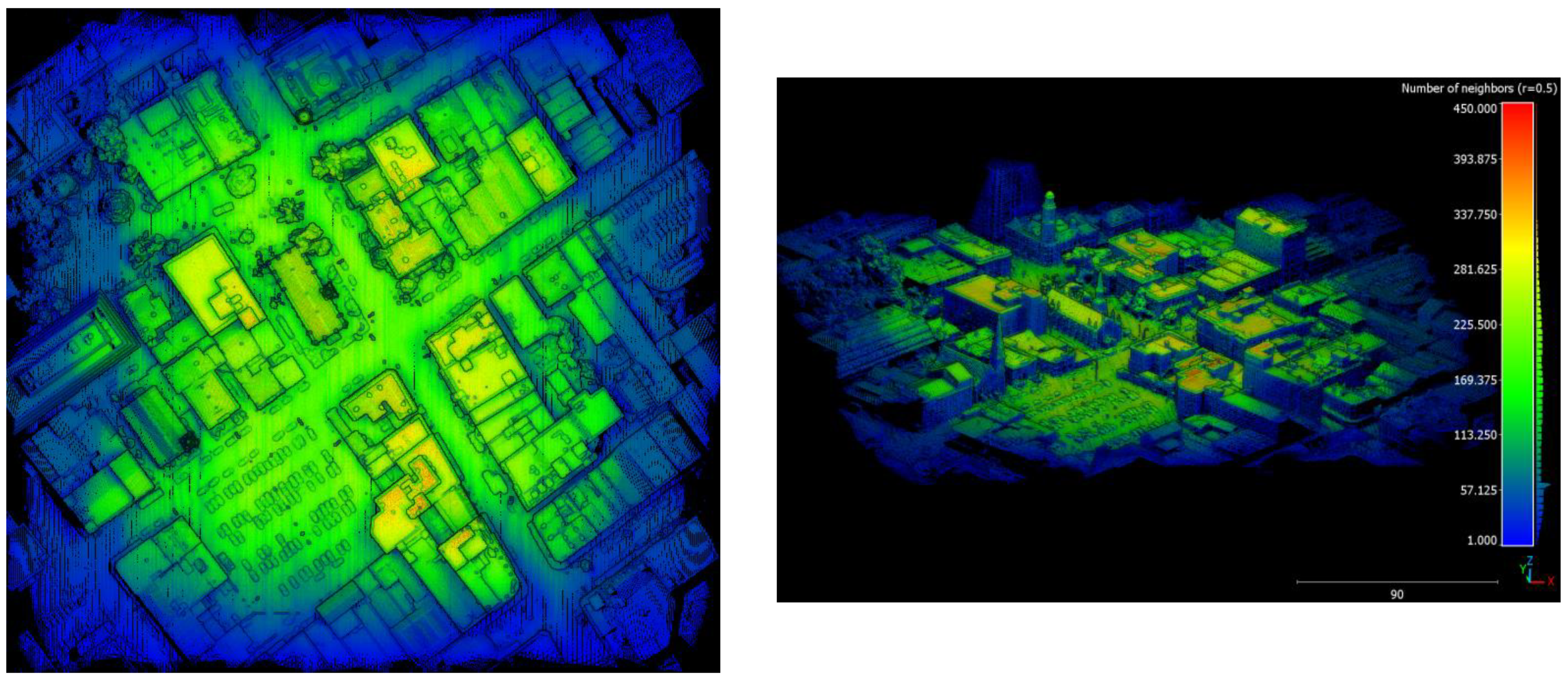
Figure 10.
Density (radius = 50 cm) of the LiDAR-based point cloud created by the Ouster LiDAR using the senseFly-based hybrid system over Launceston.
Figure 10.
Density (radius = 50 cm) of the LiDAR-based point cloud created by the Ouster LiDAR using the senseFly-based hybrid system over Launceston.
Figure 11.
Flight planning with the MAPIR camera over Launceston: seven strips and 910 images.
Figure 11.
Flight planning with the MAPIR camera over Launceston: seven strips and 910 images.
Figure 12.
Recovered camera poses and sparse point cloud for the simulated MAPIR-based multi-view image block (910 images) over Launceston (a,b). Derived dense point cloud (c,d).
Figure 12.
Recovered camera poses and sparse point cloud for the simulated MAPIR-based multi-view image block (910 images) over Launceston (a,b). Derived dense point cloud (c,d).
Figure 13.
Density (radius = 50 cm) of the LiDAR-based point cloud created by the Ouster scanner using the MAPIR-based hybrid system over Launceston.
Figure 13.
Density (radius = 50 cm) of the LiDAR-based point cloud created by the Ouster scanner using the MAPIR-based hybrid system over Launceston.
Figure 14.
Flight planning with the senseFly camera over Dortmund: five strips and 665 images.
Figure 14.
Flight planning with the senseFly camera over Dortmund: five strips and 665 images.
Figure 15.
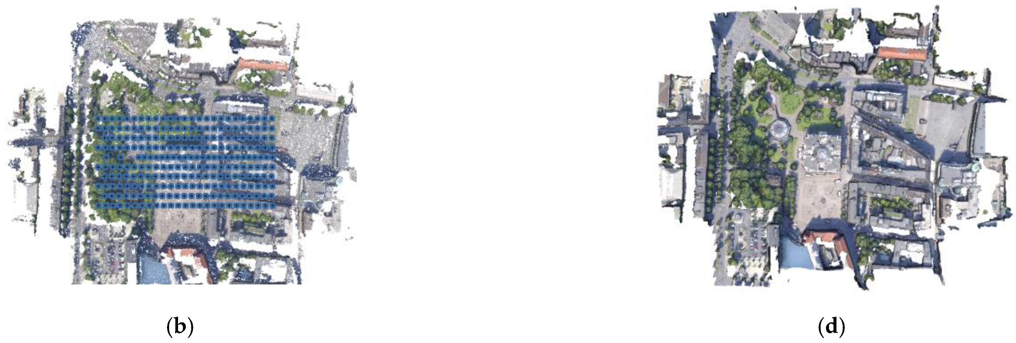
Recovered camera poses and sparse point cloud for the simulated senseFly-based multi-view image block (665 images) over Dortmund (a,b). Derived DIM point cloud (c,d).
Figure 15.
Recovered camera poses and sparse point cloud for the simulated senseFly-based multi-view image block (665 images) over Dortmund (a,b). Derived DIM point cloud (c,d).
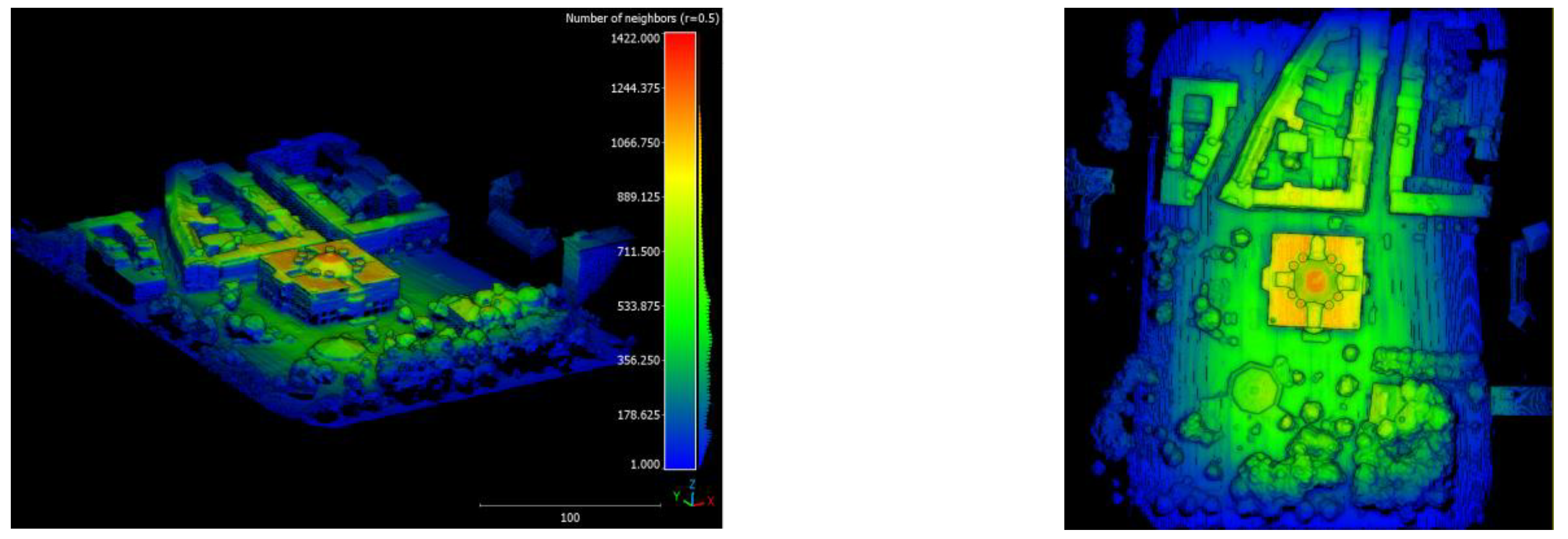
Figure 16.
Density (radius = 50 cm) of the LiDAR-based point cloud created by the Ouster scanner using the senseFly-based hybrid system over Dortmund.
Figure 16.
Density (radius = 50 cm) of the LiDAR-based point cloud created by the Ouster scanner using the senseFly-based hybrid system over Dortmund.
Figure 17.
Flight planning with the MAPIR camera over Dortmund: ten strips and 1250 overlapping multi-view images.
Figure 17.
Flight planning with the MAPIR camera over Dortmund: ten strips and 1250 overlapping multi-view images.
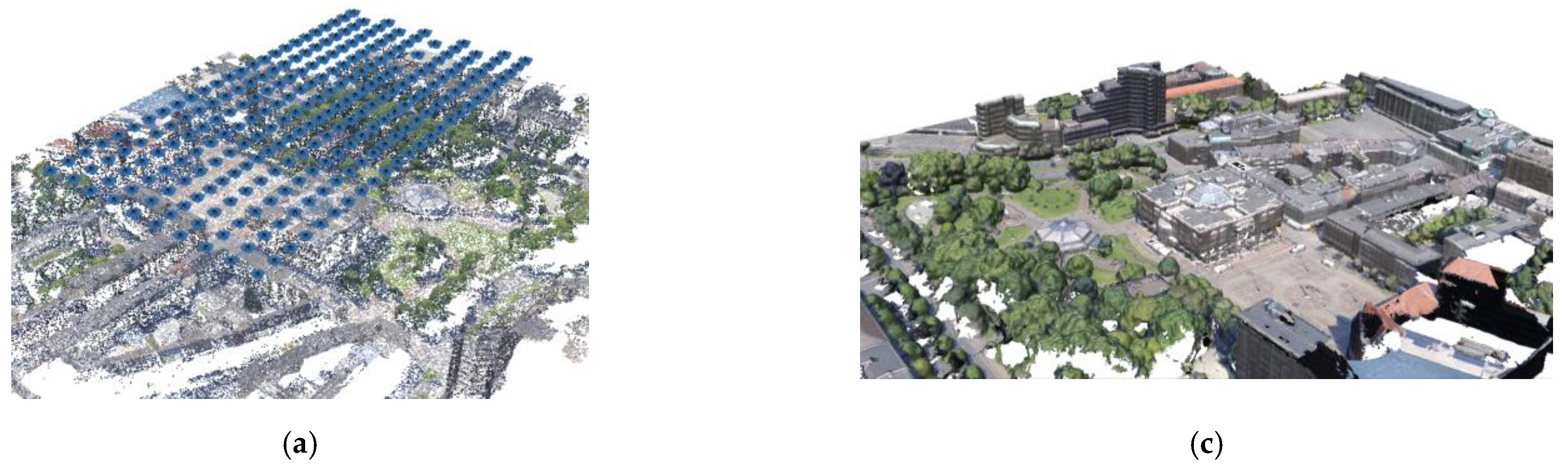
Figure 18.
Recovered camera poses and sparse point cloud for the simulated MAPIR-based multi-view image block (1250 images) over Dortmund (a,b). Derived dense point cloud (c,d).
Figure 18.
Recovered camera poses and sparse point cloud for the simulated MAPIR-based multi-view image block (1250 images) over Dortmund (a,b). Derived dense point cloud (c,d).
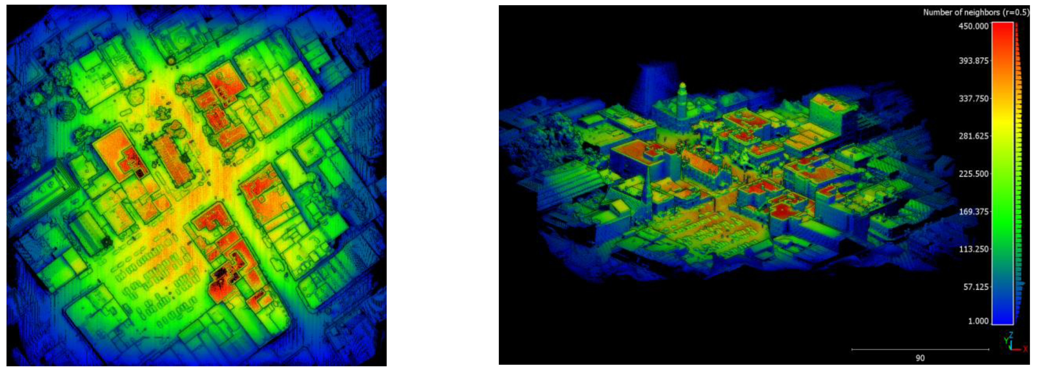
Figure 19.
Density (radius = 50 cm) of the LiDAR-based point cloud created by the Ouster LiDAR using the MAPIR-based hybrid system over Dortmund.
Figure 19.
Density (radius = 50 cm) of the LiDAR-based point cloud created by the Ouster LiDAR using the MAPIR-based hybrid system over Dortmund.
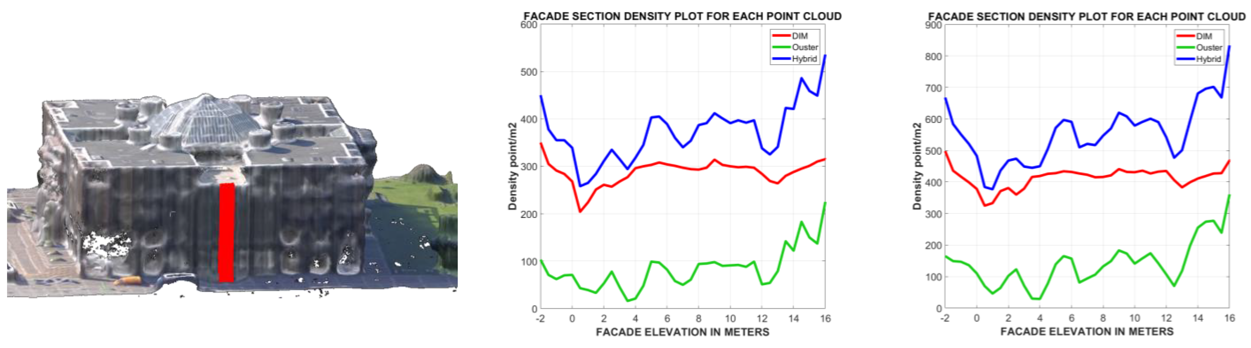
Figure 20.
Plots of density profiles on a building façade in Dortmund.
Figure 20.
Plots of density profiles on a building façade in Dortmund.
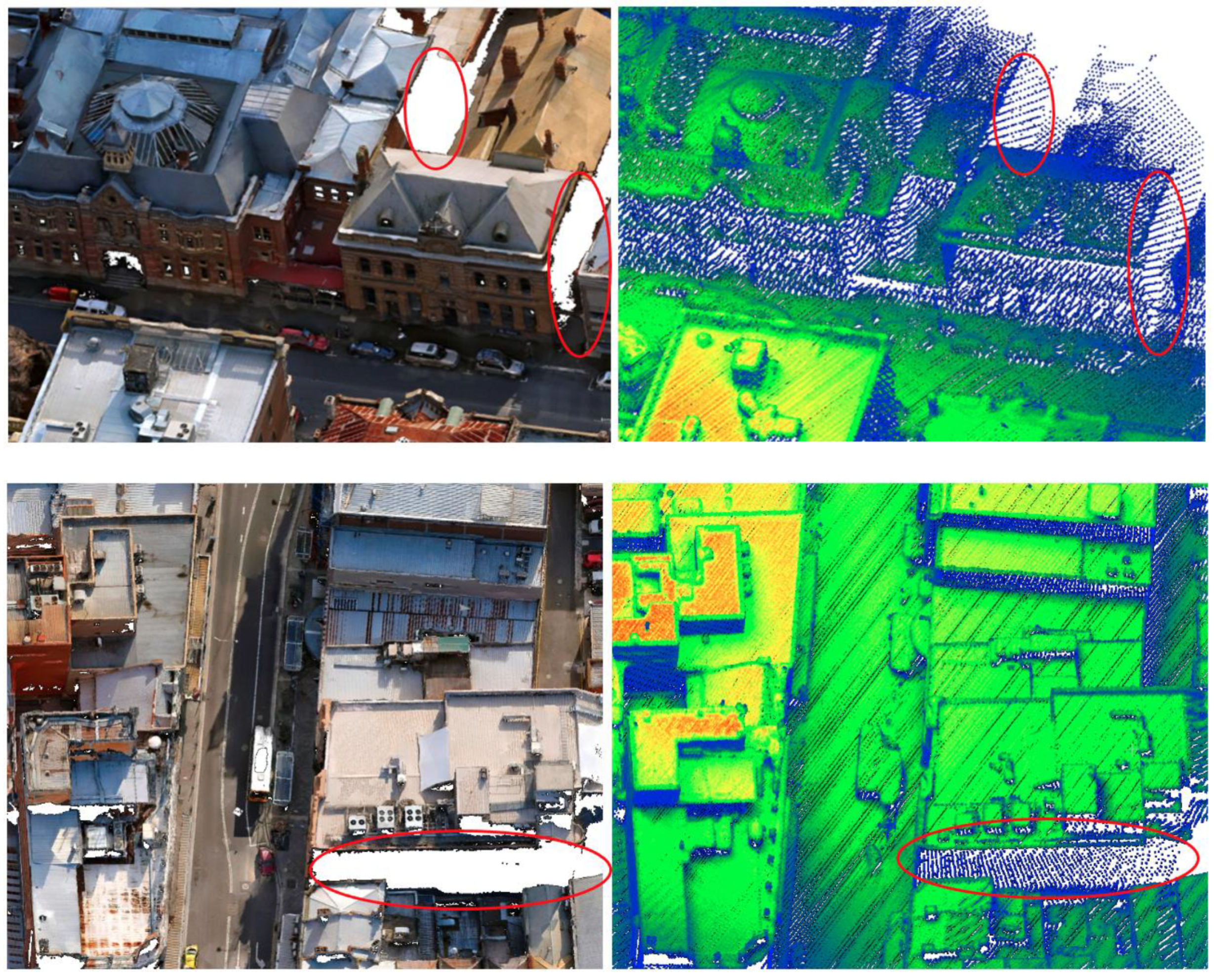
Figure 21.
Photogrammetric point cloud (left) and LiDAR point cloud (right) with highlighted areas of complementarity between the two datasets.
Figure 21.
Photogrammetric point cloud (left) and LiDAR point cloud (right) with highlighted areas of complementarity between the two datasets.
Figure 22.
A comparison of the point density and improvement after integrating point clouds from LiDAR and DIM. For both hybrid sensors, the point clouds shown have the same minimum and maximum limits.
Figure 22.
A comparison of the point density and improvement after integrating point clouds from LiDAR and DIM. For both hybrid sensors, the point clouds shown have the same minimum and maximum limits.
Table 1.
Specifications of some commercial multi-view camera systems for UAV platforms.
Table 1.
Specifications of some commercial multi-view camera systems for UAV platforms.
| | Resolution | Sensors | Size | Weight |
|---|
| Viewprouav VO305 | 305 MPx | Full frame | 20 m × 20 m × 112 mm | - |
| Share 303S Pro | 305 MPx | Full frame | 200 × 200 × 125 mm | 1.4 kg |
| DroneBase N5 | 120 MPx | APS-C | 160 × 160 × 85 mm | 730 gr |
| ADTi Surveyor 5 PRO | 120 MPx | APS-C | 105 × 150 × 80 mm | 850 gr |
| Quantum-System D2M | 130 MPx | APS-C | - | 830 gr |
| JOUAV CA504R | 305 MPx | Full frame | 270 × 180 × 154 mm | 2.25 kg |
Table 2.
Main characteristics of the considered MAPIR and senseFly cameras.
Table 2.
Main characteristics of the considered MAPIR and senseFly cameras.
| Specification | MAPIR Survey3W | senseFly SODA |
|---|
| Focal length [mm] | 8.25 | 10.6 |
| Sensor [pixels] | Sony Exmor R IMX1174032 × 3024 | CMOS 1”, 5472 × 3648 |
| Pixel size [microns] | 1.55 | 2.33 |
| Field of view | 87° | 74° |
| Storage [GB] | Max 128 GB Storage | Based on external memory |
| Data exchange format | PWM, USB, HDMI, and SD | PWM, USB, HDMI, and SD |
| Shutter speed | Global Shutter 1/2000 to 1 min | Global Shutter 1/500–1/2000 s |
| Aperture | f/2.8 | f/2.8–f/11 |
| Dimensions | 59 × 41.5 × 36 mm | 75 × 48 × 33 mm |
| Weight | 75.4 g with battery | 85 g |
| Battery | 1200 mAh Li-Ion (150 min) | No internal battery, powered by drone |
| Price | ca. EUR 400 | ca. EUR 1500 |
Table 3.
Main characteristics of the Ouster OS1-32 LiDAR sensor and its typical scanning ground footprint (right).
Table 3.
Main characteristics of the Ouster OS1-32 LiDAR sensor and its typical scanning ground footprint (right).
| LiDAR Sensor/System | Ouster OS1-32 | ![Drones 06 00314 i001]() |
| Max. Range | ≤120 m@80% reflectivity |
| Typical Range Accuracy 1σ | ±3 cm |
| Beam divergence | 0.18° (3 mrad) |
| Beam footprint | 22 cm@100 m |
| Scanning channels/beams | 32 channels |
| Output rate pts/sec. | 655,360 |
| Laser Returns | 1 per outgoing pulse |
| FOV-Vertical | 45° (±22.5°) |
| Rotation rate | 10–20 Hz |
| Angular resolution | 0.35°–2.8° |
| LiDAR mechanism | Spinning |
| LiDAR type | Digital |
| Laser Wavelength | 865 nm |
| Power consumption | 14–20 w |
| Weight | 455 g |
| Dimensions (diameter × height) | 85 × 73.5 mm |
| Operating Temperature | −20 °C to +50 °C |
| Initial price | ca. EUR 8000 |
Table 4.
Overall characteristics of the integrated camera and LiDAR sensors.
Table 4.
Overall characteristics of the integrated camera and LiDAR sensors.
| LiDAR | Ouster S1-32 |
|---|
| Number of cameras | 4 oblique + 1 nadir |
| Dimensions | 24.6 cm × 21 cm × 8 cm (MAPIR config.)
23.4 cm × 15.8 cm × 8 cm (SODA config.) |
| Focal length | 10.6 mm (SODA config.)
8.25 mm (MAPIR config.) |
| Megapixels | 12 MPx (MAPIR config.)
20 MPx (SODA config.) |
| Camera tilting | 45° (or 30°) |
| Data exchange format | USB Memory Stick |
| Expected operation time per charge | >1 h |
| Operational temperature range | 0 °C to 40 °C |
| Mass | <1 kg, with battery |
| Price | EUR <10,000 |
Table 5.
Pseudocode for the flight planning parameters.
Table 5.
Pseudocode for the flight planning parameters.
Input: the ROI shapefile, camera and LiDAR parameters, required GSD. Output: Flight plan parameters including:
UAV waypoints and save them as an array in a folder. Display planning results in the tool GUI The plot of the footprints of the images
Check input options of the overlap, height, speed, inclination angle, portrait/landscape, type of the camera, and marginal flight strips Compute the min. and max. GSD and display them in the GUI Call the function of the flight planner calculator:
Plot the ROI Define if the ROI is either elongated NS or EW Calculate the airbase B, no. of strips, no. of images, travel time, and the XYZ of the waypoints
|
Table 6.
Pseudocode for the estimation of the LiDAR point cloud on the ground.
Table 6.
Pseudocode for the estimation of the LiDAR point cloud on the ground.
Table 7.
Accuracy analyses on the two simulated image datasets over Launceston and GCP/CP distribution (right).
Table 7.
Accuracy analyses on the two simulated image datasets over Launceston and GCP/CP distribution (right).
| | RMSE_ XY (mm) | RMSE_Z (mm) | Total RMSE (mm) | |
|---|
| | senseFly-based hybrid system (nadir GSD: 1.8 cm) | ![Drones 06 00314 i002]() |
| GCPs (5) | 4.1 mm | 1.3 mm | 4.3 mm |
| CPs (7) | 4.3 mm | 1.8 mm | 4.6 mm |
| | MAPIR-based hybrid system (nadir GSD: 1.5 cm) | ![Drones 06 00314 i003]() |
| GCPs (5) | 4.4 mm | 1.0 mm | 4.5 mm |
| CPs (7) | 3.7 mm | 1.2 mm | 3.8 mm |
Table 8.
Accuracy analyses on the two simulated image datasets over Dortmund and GCP/CP distribution (right).
Table 8.
Accuracy analyses on the two simulated image datasets over Dortmund and GCP/CP distribution (right).
| | RMSE_ XY (mm) | RMSE_Z (mm) | Total RMSE (mm) | |
|---|
| | senseFly-based hybrid system | ![Drones 06 00314 i004]() |
| GCPs (6) | 2.8 mm | 0.5 mm | 2.9 mm |
| CPs (9) | 3.7 mm | 1.8 mm | 4.1 mm |
| | MAPIR-based hybrid system | ![Drones 06 00314 i005]() |
| GCPs (6) | 2.3 mm | 2.4 mm | 3.3 mm |
| CPs (9) | 4.6 mm | 3.3 mm | 5.7 mm |
Table 9.
Summary of the generated and integrated sample point clouds with the proposed hybrid systems for UAV platforms.
Table 9.
Summary of the generated and integrated sample point clouds with the proposed hybrid systems for UAV platforms.
| | First test | Second test |
|---|
| | senseFly + Ouster | MAPIR + Ouster | senseFly + Ouster | MAPIR + Ouster |
|---|
| Total DIM points | 3,165,250 | 5,516,791 | 7,523,625 | 10,818,103 |
| Total LiDAR points | 1,100,675 | 1,692,890 | 9,593,969 | 14,289,084 |
| Total Integrated | 4,265,925 | 7,209,681 | 16,912,628 | 25,107,187 |
| Density DIM | 469 ± 81 pts/m2 | 804 ± 121 pts/m2 | 338 ± 77 pts/m2 | 496 ± 120 pts/m2 |
| Density LiDAR | 188 ± 67 pts/m2 | 296 ± 102 pts/m2 | 659 ± 340 pts/m2 | 1050 ± 544 pts/m2 |
| Density Integrated | 619 ± 120 pts/m2 | 1039 ± 178 pts/m2 | 877 ± 359 pts/m2 | 1329 ± 575 pts/m2 |


