Abstract
To investigate the vibration behavior of ship-borne tethered UAVs under taut–slack conditions, the Hamilton principle is used to establish the three-dimensional dynamic equations of the ship-borne tethered UAVs while taking into account geometric nonlinearity and simplifying them into the corresponding stress wave equations. By employing the characteristic line technique to solve the stress wave equation of ship-borne tethered UAVs, it is possible to numerically determine the effects of various factors on the vibration behavior of these drones. Dimensional analysis is then used to build the experimental model, ensuring that the numerical outcomes are accurate. The findings show that the impact of equilibrium curvature connects longitudinal and transverse waves and that the geometric dispersion of stress wave propagation in the tethered cable is caused by equilibrium curvature. The standing wave takes the lead and causes subharmonic and frequency doubling components in the top tension response when the end excitation frequency is near the tethered UAVs’ natural frequency. Additionally, the cable’s center as well as its end will display the highest dynamic tension value.
1. Introduction
UAVs have been widely utilized in resource exploitation, anti-terrorism surveillance, civil aerial photography, and other sectors due to static hovering and stability. However, UAVs struggle with endurance and the wirelessly transmitted data they relay are readily hacked. To make the UAV platform operate for a long time and assure the effectiveness and safety of information transmission, it can be attached to an optoelectronic composite tether. Tethered UAVs are this kind of UAV.
Tethered UAVs have a wider range of potential applications and the benefits of lengthy hovering durations and plentiful power over regular UAVs. These benefits have led to the widespread deployment of tethered UAVs in areas such as marine emergency communication [1], forest firefighting [2], and bridge safety detection [3].
The photoelectric composite cable serves as both the power source and the information conduit for the tethered UAVs. Due to its interconnected nature, the UAV platform’s movement will have an impact on the internal strain of the tethered cable. When the strain is too high, the tethered cable will be harmed, which will also cause the tethered UAVs to malfunction. As a result, it is not sufficient to focus just on the UAV platform’s dynamic reaction when it is impacted; The way UAV platform affects the tethered cable must be taken into account. In order to guarantee the long-term functioning of tethered UAVs, it is necessary to explore their dynamic properties in a challenging environment. For tethered UAVs to operate steadily, a large number of professionals have worked on the dynamic model and control principles. Wu neglected the cable’s local bending in favor of simplifying the tethered cable to the spring-mass-damping model while creating the control algorithm for the ship-borne tethered UAVs [4]. Nicotra focused on creating a stabilizing control rule for a cable-connected aerial vehicle attached to a base station [5]. Using the UAV as a constraint at one end of the cable, Muttin simplified the ship-borne tethered UAVs system and built a nonlinear dynamic model [6]. Before optimizing UAV pathways to maintain tight tethers, Ya looked at the dynamic available wrench set and maximum maneuver acceleration [7].
Tethered cables often consist of flexible ropes with tiny diameters, making them easier to bend and having short portions. The tethered cables will swing as a result of the external wind load and UAV motion, cycling between a taut and slack condition. Because the cable’s optical fiber has inadequate bending resistance in this instance, the signal transmission will be hampered. According to certain research, the snap load in the cable is 5 times or even more than 10 times the usual tension when the mooring cable structure is under relaxation tension [8]. According to Basile Audoly’s research, a localized increase in curvature caused by the abrupt relaxation of the curvature at this end causes a burst of flexural waves, which permits a cascade failure process [9]. Tjavaras investigated the dynamic behavior of a tethered near-surface buoy subject to wave excitation and discovered that, at a threshold wave amplitude, the mooring system exhibits first zero tension, then a snapping reaction, and the buoy shows chaotic motion [10]. In addition, he discovered that the curvature may significantly alter the magnitude of the shock wave’s stress during the research of synthetic curved cables [11]. With the use of the Hamiltonian principle, Perkins was able to construct the three-dimensional dynamic equation for the moving cable and discovered that the equilibrium configuration’s nonzero curvature is what links the cable tension and velocity [12]. Two qualitatively different in-plane waveforms were discovered by Behbahani Nejad while researching elastic wave free propagation in the cable. One wave type mostly generates longitudinal deformations and propagates with a speed that is similar to that of an elastic rod, whereas the other wave type primarily induces transverse deflections and propagates with a speed that is similar to that of a taut string [13]. Additionally, he studied the forced response of an elastic cable that was infinitely long and slightly curved while being exposed to focused harmonic stimulation using the Green’s function approach. According to research, transverse excitation can produce a sizable, long-distance tension wave [14]. Lin studied the structural wave generated and propagated in the interaction between the seabed and mooring structure through the numerical solution and found that the seabed has a significant influence on the propagation of transverse waves in the cable [15].
There is currently no study on the dynamic response of ship-borne tethered UAVs under taut–slack conditions. This is due to the fact that the ship-borne tethered UAVs are impacted by ship motion at one end and attached to the UAV platform at the other end, and the boundary conditions are dynamic. In this study, a set of wave dynamics equations for the ship-borne tethered UAVs are created, and a numerical analysis of the tension and velocity of ship-borne tethered UAVs under the conditions of the ship’s heaving is carried out by the characteristic line technique. After that, the trial confirms the analyses’ findings, which form the basis for the ship-borne tethered UAVs’ design.
The remainder of the paper is organized as follows. In Section 2, the dynamic equations of ship-borne tethered UAVs are derived and then solved by the stress wave method. In Section 3, the numerical simulation is carried out to analyze the dynamic behaviors under different conditions. In Section 4, the model experiment is established to verify the former results. Finally, Section 5 concludes the paper.
2. Theoretical Analysis
2.1. Governing Equations of the Ship-Borne Tethered UAVs
A theoretical model is derived that describes the nonlinear, three-dimensional motion of ship-borne tethered UAVs. The tethered cable is considered to be a homogeneous, linearly elastic, one-dimensional continuum with negligible torsional, bending, and shear rigidities and is subject to gravity, tension, and wind forces. Figure 1 illustrates the tethered UAVs’ equilibrium configuration (dashed curve) and the dynamic configuration (solid curve) following a disturbance. The position vectors and describe the location of a material point on the cable centerline in the equilibrium and dynamic configurations, respectively. The three-dimensional dynamic response of the cable about equilibrium is projected onto the equilibrium Serret–Frenet triad composed of the unit tangent , normal , and binormal directions. Hence, , where denotes the equilibrium arc length coordinate and denotes time.
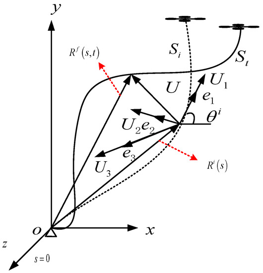
Figure 1.
Schematic diagram of tethered UAVs system.
The strain energy of the tethered UAVs in the dynamic configuration is:
where is the strain energy in the equilibrium configuration, is the equilibrium cable length, is the equilibrium cable tension distribution, is the cable cross-sectional area, and is Young’s modulus. Here, denotes the dynamic component of the Lagrangian strain measure for centerline extension.
where is the equilibrium curvature.
The gravitational potential energy of the system in the dynamic configuration is:
where is the angle between the direction and horizontal direction.
The kinetic energy of the system in the final configuration is
where is the material density of the mooring cable in the ship-borne tethered UAVs, and is the absolute velocity of each point on the tethered cable, and its expression is:
The virtual work caused by wind load is considered as
where , are the components of external force on tethered UAVs along , and directions, respectively.
Substituting those expressions into Hamilton’s principle:
The equations of motion for the ship-borne tethered UAVs are derived:
It can be obtained that the in-plane equations of motion are coupled with each other by the equilibrium curvature , and the out-of-plane equation is coupled, so only the in-plane equations of motion are discussed.
The tethered cable is fixed to the ship at its lower end and is attached to the UAV platform at its upper end. The lower end of tethered UAVs is determined by ship motion. The force diagram of the UAV platform is shown in Figure 2. The boundary condition of the upper end is derived as follows:
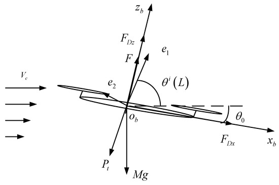
Figure 2.
Force diagram of UAV platform.
Where is the body coordinate system in the plane of the UAV, is the horizontal wind speed, is the total lift of the UAV, is the inclination between and the horizontal direction, is the included angle between and the horizontal direction, is the gravity of the UAV, is the total tension of the mooring cable to the tethered UAVs, and and are the aerodynamic force received by the UAV in and directions, respectively. The expressions are:
where is the component of in and is the component of in , and the expressions are:
Decomposing the force on the UAV along directions, the boundary condition of the upper end is:
2.2. Stress Wave Solution of Ship-Borne Tethered UAVs’ Motion Equations
The tangential, normal, and sub-normal dynamic equations of ship-borne tethered UAVs are obtained by the Hamilton principle as shown in Equations (17)–(19):
The dynamic strain, equilibrium tension, and equilibrium curvature are as follows:
where A is the cross-section area of the cable, ρ is the material density of the cable, and P0 is the horizontal component of the equilibrium tension.
In the small-curvature hypothesis , Equations (21) and (22) can be changed into:
By substituting Equations (23) and (24) into Equations (17)–(19), the following results are obtained:
Among them,
It can be obtained from Equations (25)–(27) that the dynamic equation of the auxiliary normal tethered UAVs is the tension string equation, so we mainly focus on the tangential and normal dynamic equations in the plane.
The characteristic line is an optimized finite difference method. When the characteristic line equation and the compatibility relationship are determined, the solution of the partial differential equations can be reduced to the corresponding ordinary differential equations, which are much easier to solve. The characteristic line method can give clear physical images of wave propagation, and can directly deal with wave images with discontinuities. The characteristic line method is widely used in the analysis of the KP equation [16] and explosion equations [17].
According to the linear elastic assumption, the tangential strain and normal strain are [11]:
In the case of neglecting the external force of air acting on the cable, substituting Equations (28) and (29) into Equations (25) and (26), the dynamic equation is obtained:
Because are derivatives of about , and are monotonic and continuous, we have a compatible equation:
Two algebraic equations are obtained from Equations (30)–(33) by the indefinite line method:
As there is more than one characteristic line, the solutions of Equations (34) and (35) are not unique, and the determinants are zero:
According to Equations (36) and (38), the velocities of the longitudinal wave and transverse wave in tethered UAVs are as follows:
Substituting Equations (40) and (41) into Equations (37) and (39), respectively, the compatibility relationship along the characteristic line is obtained:
It can be obtained from Equations (42) and (43) that the compatibility relationship along the characteristic line contains and , so the phase velocity of the wavefront is not constant. It describes the dispersion characteristics of a transverse wave and a longitudinal wave in ship-borne tethered UAVs. The coefficients of these terms are related to the equilibrium curvature . It can be seen that even if the cable has a linear elastic constitutive relation, the internal stress wave will propagate. However, the phenomenon of geometric dispersion caused by the geometric size factor still appears.
Generally speaking, the velocity of a longitudinal wave is greater than that of a transverse wave. For each point on the tethered cable, when the longitudinal wave arrives first and the transverse wave does not arrive, it should only show the characteristics of a longitudinal wave, and when the transverse wavefront arrives, the position should show the coupling characteristics of a transverse wave and longitudinal wave.
Considering the influence of the ship’s heave on the tethered UAVs, the lower end of the ship-borne tethered UAVs moves in a simple harmonic direction, so the lower boundary conditions of the stress wave are shown in Equations (44) and (45):
Among them, Ae is the excitation amplitude of the ship to the tethered UAVs, and ω is the excitation circle frequency of the ship to the tethered UAVs.
The top of the ship-borne tethered UAV keeps its balance by adjusting its lift at all times, so the upper boundary conditions are as follows:
It can be obtained from the compatibility equation that it is challenging to solve the analytical solution, which is solved by the characteristic line numerical method. The difference method is used to establish the discrete scheme of the compatible equation.
Lower boundary:
Upper boundary:
Interior point:
The difference scheme of boundary points and interior points is shown in Figure 3.
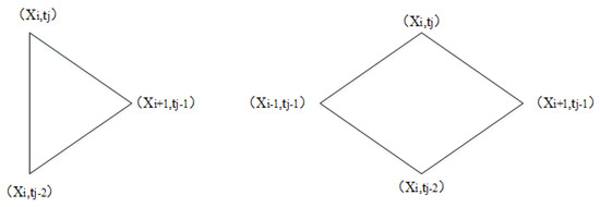
Figure 3.
Difference scheme of boundary point and interior point.
3. Numerical Simulation
From the differential format, it can be seen that the dynamic strain in the tethered cable is influenced by the material parameters of the cable, the initial pretension, and the bottom excitation frequency and amplitude. In order to investigate the effects of parameters such as the length, material parameters, excitation frequency, and excitation amplitude on the dynamic tension of the cable, the working conditions shown in Table 1 are designed. According to studies [18,19], the ship’s heave motion can be approximated as a simple harmonic, so the excitation frequency of the bottom end of the tethered UAVs is set between 0.1 Hz and 0.3 Hz with an interval of 0.05 Hz. The excitation amplitude ranges from 1 m to 5 m with 1 m. The linear density of the cable is 0.02 kg/m (not changing with the cross-sectional area of the cable).

Table 1.
Parameter and condition setting.
Taking condition 1.1 as an example, the excitation amplitude Ae = 2 m and the excitation frequency = 0.1 Hz, 0.15 Hz, 0.2 Hz, 0.25 Hz, 0.3 Hz. The relationship between the maximum absolute value of the tangential, normal, and dynamic strain with frequency and the cable’s body coordinates is shown in Figure 4.
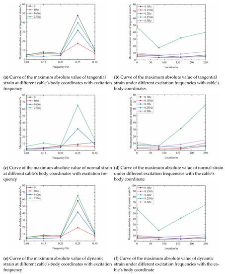
Figure 4.
The relationship between the maximum absolute value of tangential (a,b), normal (c,d), and dynamic strain (e,f) with frequency and the cable’s body coordinates.
From Figure 4, it can be obtained that with constant pretension and excitation amplitude, the maximum absolute value of the top dynamic strain is less than that of the bottom dynamic strain at low excitation frequencies, and the maximum absolute value of the top dynamic strain is slightly more than that of the bottom dynamic strain at high excitation frequencies. However, at the excitation frequency of 0.25 Hz, an anomaly occurs. It can be seen that the maximum absolute value of tangential, normal, and dynamic strain is significantly larger than those at other excitation frequencies regardless of the cable’s body coordinates.
In order to analyze the anomalies appearing at the excitation frequency of 0.25 Hz, the excitation frequency change interval is shortened to 0.1 Hz, and the top dynamic strain time course curve is subjected to spectral analysis with a sampling frequency of 30 Hz and 2048 sampling points. The number and magnitude of the amplitudes obtained from the spectrum analysis are as shown in Figure 5, and the frequency spectrum curves according to different excitation frequencies are as shown in Figure 6.
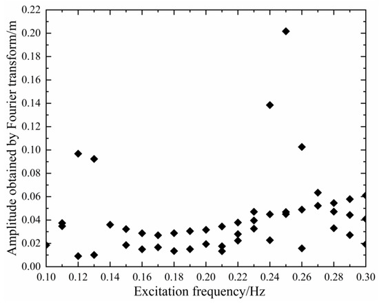
Figure 5.
Variation curves of number and amplitude with excitation frequency obtained by spectral analysis of dynamic strain at the top.
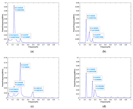
Figure 6.
The number and magnitude of the amplitudes and frequency response curve of top dynamic strain at different excitation frequencies: (a) = 0.13 Hz, Ae = 2 m; (b) = 0.18 Hz, Ae = 2 m; (c) = 0.24 Hz, Ae = 2 m; (d) = 0.30 Hz, Ae = 2 m.
When the tethered UAV hovers, the structure is similar to the cable-stayed bridge [20]. It can be approximated that the natural frequency of the tethered UAVs in the hovering state is . This equation is substituted by the parameters of working condition 1.1; the first natural frequency of the hovering tethered UAVs is predicted to be about 0.1235 Hz. Figure 4 shows that a rich dynamics phenomenon emerges when the excitation frequency crosses the first and second natural frequencies. Figure 5a shows that when the excitation frequency approaches the first natural frequency, the amplitude jumps from the single-periodic component to the multi-periodic component, and subharmonic responses, the multiply periodic response, and subharmonic response appear. Subsequently, the excitation frequency moves away from the intrinsic frequency, and in the response of Figure 5b, it can be seen that in addition to the components of the excitation frequency, there are also components of the first and second natural frequencies, and the subharmonic response disappears. The amplitude jumps again when the excitation frequency is close to the second natural frequency, and the multiplicative periodic and subharmonic responses appear. When the excitation frequency is far from the second natural frequency, the first and second natural frequencies and the excitation frequency components exist in addition to the excitation frequency, and the multiply periodic response disappears. In order to avoid the amplitude jump phenomenon, the first natural frequency of the tethered UAVs must be made as large as possible by changing the relevant parameters, such as the length of the tethered cable and the tension provided at the tip, thus avoiding the excitation frequency close to the natural frequency.
Figure 7 shows the curve of dynamic tension of the top with time in the first few seconds. The time of 0 s is the first time that the bottom of the tethered UAV is excited. It can be seen that in the first few seconds, there are two sudden changes in the top dynamic tension. The first is because the longitudinal wave generated by the bottom excitation reaches the top, and the second is because the transverse wave reaches the top. Because of the existence of the transverse wave, the shape of the cable is changed, resulting in sudden changes in the dynamic tension. In the second change, the dynamic tension increases rapidly, then decreases, and then the top dynamic tension is affected by both transverse and longitudinal waves.
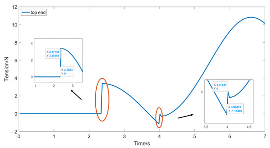
Figure 7.
The curve of the dynamic tension of the cable at the top with time (0 to 7 s) under = 0.18 Hz, Ae = 2 m.
Figure 8 shows the distribution of the dynamic tension in the cable with time and space for different excitation frequencies. It can be found that the variation in the cable’s dynamic tension consists of both standing waves and traveling waves. When the excitation frequency is close to the natural frequency, the standing wave dominates and forms a large response at the end of the tethered UAV. Moreover, when the excitation frequency is far from the natural frequency, the traveling wave dominates, and the end response of the tethered UAV is smaller.
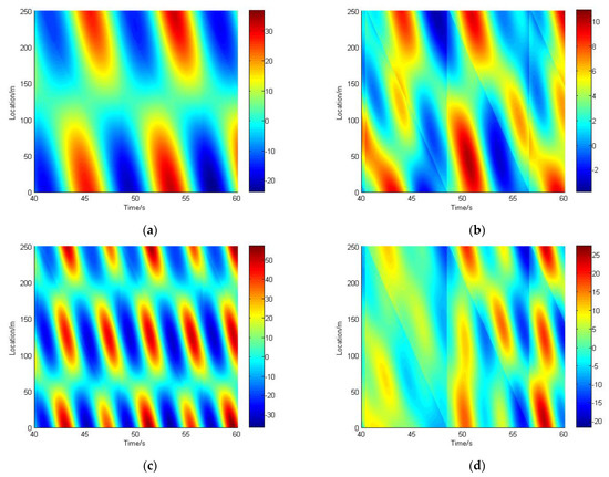
Figure 8.
Temporal and spatial distribution of dynamic cable tension (Unit: N) under different excitation frequencies: (a) = 0.13 Hz, Ae = 2 m; (b) = 0.18 Hz, Ae = 2 m; (c) = 0.24 Hz, Ae = 2 m; (d) = 0.30 Hz, Ae = 2 m.
It can be seen from Figure 8b,c that the maximum dynamic tension occurs not only at the upper and lower end of the cable but also in the middle of the cable at a certain time.
Then, the variation in dynamic cable tension with excitation amplitude is analyzed. Taking working condition 1.1 as an example, the excitation frequency = 0.15 Hz and the excitation amplitude Ae = 1 m, 2 m, 3 m, 4 m, and 5 m. The strain versus time curves at different locations are shown in Figure 9.
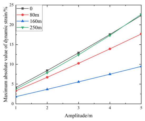
Figure 9.
Variation curve of the maximum absolute value of dynamic strain with excitation amplitude at different positions.
It can be seen from Figure 9 that under the same excitation frequency, with the increase in excitation amplitude, the maximum absolute value of dynamic strain at each point of the tethered cable gradually increases.
Then, the variation in dynamic tension in the cable with cable length and pretension is analyzed. Taking working conditions 1.2 and 1.3 as examples, under the excitation frequency = 0.12 Hz and the excitation amplitude Ae = 2 m, the distribution of dynamic tension with time and cable position under the two working conditions is shown in Figure 10.
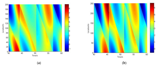
Figure 10.
Temporal and spatial distribution of dynamic cable tension (Unit: N) under excitation frequency = 0.12 Hz and excitation amplitude Ae = 2 m: (a) working condition 1.2; (b) working condition 1.3.
It can be seen from Figure 10 that by reducing the length of the cable and increasing the pretension, the sudden increase in tension and end point aggregation caused by the excitation frequency close to the natural frequency can be effectively avoided. Because the tethered UAVs need to maintain a certain height when working, increasing the lift of the UAV is an effective way to keep the tethered UAVs operating for a long time.
Finally, the variation in dynamic tension with cross-sectional cable area and elastic modulus is analyzed. Taking working conditions 1.4 and 1.5 as examples, under the excitation frequency = 0.19 Hz and the excitation amplitude Ae = 2 m, the distribution of dynamic tension with time and cable position under these two working conditions is shown in Figure 11.
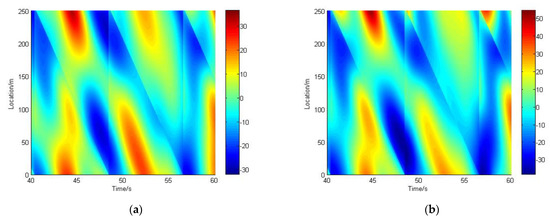
Figure 11.
Temporal and spatial distribution of dynamic cable tension (Unit: N) under excitation frequency = 0.19 Hz and excitation amplitude Ae = 2 m: (a) working condition 1.4; (b) working conditions 1.5.
When the linear density remains unchanged, increasing the elastic modulus and the cable’s cross-sectional area will increase the longitudinal wave’s velocity. It can be seen from Figure 11 that the maximum amplitude tends to increase.
4. Experiment
In order to conduct experimental research on tethered UAVs, it is necessary to determine the experimental model and experimental devices. According to the theorem, the relationship between the parameters of the model and the prototype is given by the implicit function in Equation (56):
The dimensional matrix is shown in Table 2.
Table 2.
Dimensional matrix.
Five independent criteria are identified as follows:
In addition, is:
Because the forces on the tethered UAVs are mainly analyzed, the dimensionless equation is changed to:
The parameters with subscript represent the model’s parameters, and the parameters with subscript represent the parameters of the prototype. The prediction equation is:
Assuming that the scale ratio of length is and the Young’s moduli of the prototype and model are the same, the scale ratio relationship between model and prototype parameters can be obtained, as shown in Table 3.
Table 3.
Relationship between the scale ratio of model and prototype parameters.
As shown in Figure 12, a simplified model is designed to study the influence of the frequency of periodic displacement excitation of the mooring point on the tension in the tethered UAVs. The frequency converter applies vertical harmonic displacement excitation at the lower end of the cable through the fixed pulley, the upper and lower tension sensors measure the tension at the end of the mooring line, and five FBG sensors are used to measure the strain at all parts of the cable. The UAV platform keeps hovering, and the cable keeps a small curvature. Because it is difficult to meet all the scale conditions, it is mainly to ensure that the material parameters of the prototype and model cable are the same. Model and prototype physical parameters of the tethered UAVs and cables are shown in Table 4, and an experimental diagram of the tethered UAVs model is shown in Figure 13.
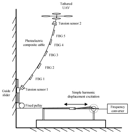
Figure 12.
Schematic diagram of end excitation model test of the tethered UAV.
Table 4.
Model and prototype physical parameters.
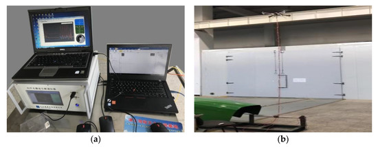
Figure 13.
Sensor data analysis equipment (a) and experimental diagram of the tethered UAV model (b).
When the amplitude of the crank slider mechanism is 0.1 m, the excitation frequency is changed to obtain the time-varying curves of the tension at the bottom and top of the tethered UAVs, as shown in Figure 14.
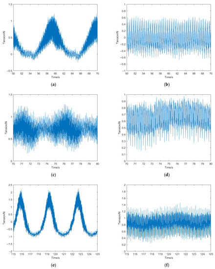
Figure 14.
The curve of the dynamic tension of cable at the bottom and top of the tethered UAV. (a) bottom, = 0.1 Hz, Ae = 0.1 m; (b) top, = 0.1 Hz, Ae = 0.1 m; (c) bottom, = 0.2 Hz, Ae = 0.1 m; (d) top, = 0.2 Hz, Ae = 0.1 m; (e) bottom, = 0.3 Hz, Ae = 0.1 m; (f) top, = 0.3 Hz, Ae = 0.1 m.
The distribution of maximum dynamic tension of tethered UAVs along with different cable positions under different excitation frequencies is shown in Figure 15.
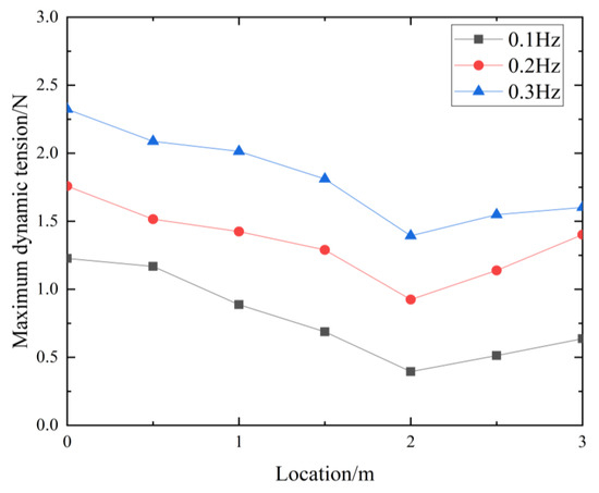
Figure 15.
Distribution of maximum dynamic tension of tethered UAVs along with different positions of cable under different excitation frequencies.
The spectrum of the dynamic tension at the top under different excitation frequencies is shown in Figure 16.
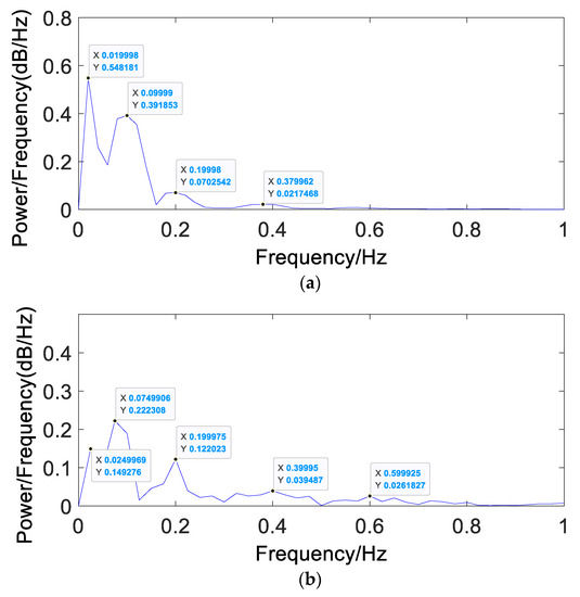
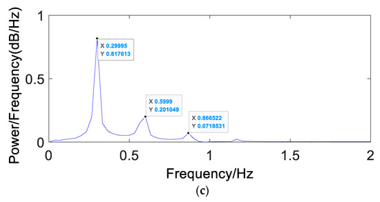
Figure 16.
The spectrum of the dynamic tension at the top under different excitation frequencies: (a) = 0.1 Hz, Ae = 0.1 m; (b) = 0.2 Hz, Ae = 0.1 m; (c) = 0.33 Hz, Ae = 0.1 m.
It can be seen that the bottom end excitation will lead to two and three times the fundamental frequency components of the top tension, and there is a subharmonic response of the top tension at the excitation frequencies of 0.1 Hz and 0.2 Hz. At the same time, it can be seen from Figure 15 that when the excitation frequency remains unchanged, the maximum dynamic tension at different positions of the tethered UAVs system does not increase nonlinearly but shows a trend of increasing fluctuation, which is consistent with the theoretical results.
5. Conclusions
An approach based on stress waves is suggested for resolving the dynamic equations of tethered UAVs. The motion differential equations of ship-borne tethered UAVs are used to create the related stress wave equations. It is discovered that the geometric dispersion of stress waves brought on by equilibrium curvature happens during the cable propagation process. The findings reveal that:
- (1)
- When the longitudinal wave or shear wave first arrives, the dynamic tension of the tethered UAV will suddenly change. It is worth noting that when the shear wave first arrives, because the shear wave will change the shape of the cable, the dynamic tension will suddenly change.
- (2)
- The standing wave takes the leading position and the tethered UAVs exhibit rich, dynamic behavior when the final excitation frequency is close to their native frequency. The top tension response will also contain subharmonic and frequency doubling components in addition to the excitation frequency component. When the excitation frequency deviates from the natural frequency, the traveling wave takes the lead and the subharmonic component vanishes.
- (3)
- The maximum dynamic tension of the tethered cable will appear not only at the upper and lower ends of the cable, but also in the middle of the cable.
- (4)
- By reducing the cable length and increasing the pretension, the sudden increase in tension and the aggregation of end points caused by the excitation frequency close to the natural frequency can be effectively avoided. Because the tethered UAVs needs to maintain a certain height when working, increasing the lift of the UAV is an effective way to keep the UAV working for a long time.
- (5)
- In the model experiment, when the excitation frequency is constant, the maximum dynamic tension at different positions of the tethered UAV system fluctuates and increases, consistent with the theoretical results.
Author Contributions
Y.T.: Conceptualization, Methodology, Software, Formal Analysis, Validation, Writing—Original Draft; S.Z.: Funding Acquisition, Project Administration, Writing—Review and Editing. All authors have read and agreed to the published version of the manuscript.
Funding
This research was funded by the National Natural Science Foundation of China (51479136) and the Natural Science Foundation of Tianjin City (17JCYBJC18700) and the APC was funded by Tianjin University.
Data Availability Statement
The data presented in this study are available on request from the corresponding author. The data are not publicly available due to privacy.
Conflicts of Interest
The authors declare that they have no known competing financial interests or personal relationships that could have influenced the work reported in this paper.
Abbreviations
| arc coordinate | |
| tethered UAVs’ equilibrium configuration | |
| tethered UAVs’ dynamic configuration | |
| the equilibrium vector | |
| the dynamic vector | |
| unit tangent | |
| unit normal | |
| unit binormal | |
| cable’s dynamic response | |
| equilibrium configuration’s strain energy | |
| equilibrium cable length | |
| equilibrium cable tension distribution | |
| cable cross-sectional area | |
| Young’s modulus | |
| Lagrangian strain | |
| equilibrium curvature | |
| angle between and horizontal direction | |
| cable’s material density | |
| the absolute velocity of the tethered cable | |
| external force on tethered UAVs along | |
| external force on tethered UAVs along | |
| external force on tethered UAVs along | |
| body coordinate in the plane | |
| horizontal wind speed | |
| total lift of the UAV | |
| angle between and the horizon | |
| angle between and the horizon | |
| gravity of the UAV | |
| mooring cable to tethered UAV’s total tension | |
| UAV’s aerodynamic force in | |
| UAV’s aerodynamic force in | |
| component of in | |
| component of in | |
| P0 | horizontal component of |
| tangential strain | |
| normal strain | |
| Ae | excitation amplitude (ship to tethered UAV) |
| ω | excitation circle frequency(ship to tethered UAV) |
| pretension | |
| cable’s length | |
| cable’s diameter |
References
- Xu, Z. Application Research of Tethered UAVs Platform in Marine Emergency Communication Network. J. Web Eng. 2021, 20, 491–512. [Google Scholar] [CrossRef]
- Viegas, C.; Chehreh, B.; Andrade, J.; Lourenço, J. Tethered UAVs with Combined Multi-rotor and Water Jet Propulsion for Forest Fire Fighting. J. Intell. Robot. Syst. 2022, 104, 21. [Google Scholar] [CrossRef]
- Wang, H.F.; Zhai, L.; Huang, H.; Guan, L.M.; Mu, K.N.; Wang, G.P. Measurement for cracks at the bottom of bridges based on tethered creeping unmanned aerial vehicle. Autom. Constr. 2020, 119, 103330. [Google Scholar] [CrossRef]
- Yang, W. Design and Control Algorithm for Moored Ship-borne Unmanned Aerial Vehicle with Large Load; Harbin Institute of Technology: Harbin, China, 2018. [Google Scholar]
- Nicotra, M.M.; Naldi, R.; Garone, E. Nonlinear control of a tethered UAV: The taut cable case. Automatica 2017, 78, 174–184. [Google Scholar] [CrossRef]
- Muttin, F. Umbilical Deployment modeling for tethered UAVs Detecting Oil Pollution from Ship. Appl. Ocean. Res. 2011, 33, 332–343. [Google Scholar] [CrossRef]
- Liu, Y.; Zhang, F.; Huang, P.; Zhang, X. Analysis, planning and control for cooperative transportation of tethered multi-rotor UAVs. Aerosp. Sci. Technol. 2021, 113, 106673. [Google Scholar] [CrossRef]
- Zhang, S.X.; Tang, Y.G.; Liu, X.J. Experimental Investigation of Nonlinear Dynamic Tension in Mooring Lines. J. Mar. Sci. Technol. 2012, 17, 181–186. [Google Scholar] [CrossRef]
- Audoly, B. Fragmentation of Rods by Cascading Cracks: Why Spaghetti Does Not Break in Half. Phys. Rev. Lett. 2005, 95, 095505. [Google Scholar] [CrossRef] [PubMed]
- Tjavaras, A.A.; Zhu, Q.; Liu, Y.; Triantafyllou, M.S.; Yue, D.K.P. The mechanics of highly-extensible cables. J. Sound Vib. 1998, 213, 709–737. [Google Scholar] [CrossRef]
- Tjavaras, A.A.; Triantafyllou, M.S. Shock Waves in Curved Synthetic Cables. J. Eng. Mech. 1996, 122, 308–315. [Google Scholar] [CrossRef]
- Perkins, N.C.; Mote, C.D. Three-dimensional Vibration of Travelling Elastic Cables. J. Sound Vib. 1987, 114, 325–340. [Google Scholar] [CrossRef]
- Behbahani-Nejad, M.; Perkins, N.C. Freely Propagating Waves in Elastic Cables. J. Sound Vib. 1996, 196, 189–202. [Google Scholar] [CrossRef]
- Behbahani-Nejad, M.; Perkins, N.C. Harmonically forced wave propagation in elastic cables with small curvature. J. Sound Vib. 1997, 119, 390. [Google Scholar] [CrossRef]
- Chen, L.; Basu, B. A numerical Study on In-plane Wave Propagation in Mooring cables. Procedia Eng. 2017, 173, 934–939. [Google Scholar] [CrossRef]
- Xin, Y.; Sun, Z.Y. Unconventional characteristic line for the nonautonomous KP equation. Appl. Math. Lett. 2020, 100, 106047. [Google Scholar]
- Wang, H.F.; Liu, Y.; Bai, F.; Yan, J.B.; Li, X.; Huang, F.L. A quasi-isentropic model of a cylinder driven by aluminized explosives based on characteristic line analysis. Def. Technol. 2022, 18, 1979–1999. [Google Scholar] [CrossRef]
- Xie, N.; Cheng, J.; Gao, H.Q. Simulation of motion time histories for ship in the seaway. J. Ship Mech. 1998, 2, 30–38. [Google Scholar]
- Li, J.D. Ship Seakeeping; National Defense Industry Press: Arlington, Virginia, 1981; p. 7. [Google Scholar]
- Simpson, A. Determination of the Natural Frequencies of Multiconductor Overhead Transmission Lines. J. Sound Vib. 1972, 20, 417–449. [Google Scholar] [CrossRef]


Publisher’s Note: MDPI stays neutral with regard to jurisdictional claims in published maps and institutional affiliations. |
© 2022 by the authors. Licensee MDPI, Basel, Switzerland. This article is an open access article distributed under the terms and conditions of the Creative Commons Attribution (CC BY) license (https://creativecommons.org/licenses/by/4.0/).