Drone-Based Atmospheric Soundings Up to an Altitude of 10 km-Technical Approach towards Operations

Abstract

Currently, the main in situ upper air database for numerical weather prediction relies on radiosonde and aircraft-based information. Typically, radiosondes are launched at specific sites daily, up to four times per day, and data are distributed worldwide via the GTS net. Aircraft observations are limited to frequent flight routes, and vertical profiles are provided in the vicinity of large cities. However, there are large areas with few radiosonde launches, in particular above the oceans and in the polar areas. In this article, the development and technical details of the unmanned aerial system LUCA (Lightweight Unmanned high Ceiling Aerial system) are described. LUCA has the potential to complement radiosonde and aircraft-based observations up to 10 km in altitude. The system ascends and descends (by electrical power) in spiral trajectories and returns to the launching site. This article discusses the requirements for obtaining high data availability under mid-European and Antarctic conditions, with highly automated take-offs and landings under high surface winds, the capacity to deal with icing, and the ability to operate under high wind speeds. The article presents technical solutions for the design and construction of the system and demonstrates its potential.

1. Introduction

Globally, numerical simulations for weather forecasts and analyses require atmospheric data as input parameters. As with most data origins of satellites, in situ observations are crucial parts of the global observing system, as hey validate and calibrate remote sensing products and observe the health of global observing system components with independent measurements. In the long-term, in situ data are important for the WMO’s (World Meteorological Organization, United Nations) global reference upper air network (GRUAN [1]) for climate watch. Focusing on in situ measurements, radiosondes, usually launched from one to four times a day, and airliner observations denote the backbone of the upper air observations, providing reliable weather data for numerical weather prediction. The global coverage of radiosonde stations is illustrated in (Figure 1a), where red dots indicate radiosonde stations, and the underlying color represents the (logarithmic) number of stations within 500 km of the vicinity. An exemplaric daily coverage of aircraft-based observations (vertical profiles) is shown in (Figure 1b); one has to keep in mind that vertical profiles are only measured in the vicinity of airports.

There are large areas with little data, in particular above the oceans and in the Antarctic. However, more data lead to improved numerical simulations of both local and worldwide weather, and in particular in determining the boundary layer altitude capped by a temperature inversion [4,5], which is of high interest for, e.g., energy meteorology and the transport of pollutants [6,7].

1.1. Why Do We Need Atmospheric Soundings with UAS?

In line with the technical achievements of uncrewed aerial system(s) (UAS), a growing community is involved in performing measurements with UAS. Unmanned aerial system(s) (UAS), also called drones and remotely piloted aircraft systems (RPAS), unmanned aerial vehicle(s) (UAV) are flexible tools that complement traditional radiosonde and airliner measurements, at least up to certain altitudes. In Sun et al. [8], for a mission on the research vessel Polarstern to the Weddell Sea in the Antarctic, additional data on radiosondes and UAS (up to altitudes of 1.1–1.7 km) improved the numerical simulations for distances of up to 300 km. However, they also stated that UAS measurements at higher altitudes would be more beneficial.

Therefore, during intensive meteorological campaigns, data from additional radiosondes or tethersondes were already gathered and included in numerical weather predictions (NWP) as, for example, in large campaigns during Project DACCIWA [9] or during the year of polar prediction [10].

The obvious advantage of using UAS for atmospheric in situ observations is the ability to return to a defined location. This leads to the ability to reuse sensors and leave less waste in the environment, which might become economically relevant in the future. In addition to the economical/ecological aspects, UAS can also measure in remote areas to fill the gap in the in situ observation network [11]. The use of UAS for operational meteorology has been discussed and implemented in the private sector in central Europe [12]. The World Meteorological Organization (WMO) is aware of the chances and coordinates of a worldwide UAS demonstration campaign, which will likely provide deep insight into the current status of UAS for operational meteorology. Nevertheless, UAS technologies are still growing for such applications, as their use in adverse weather conditions is being investigated [13], and the altitude that UAS can reach depends strongly on the size and weight and will not be comparable to radiosonde altitudes in the near future.

1.2. State-of-the-Art Atmospheric Soundings with UAS

Different systems have been developed to produce additional data similar to the classical radiosondes or dropsondes and vertical profiles from airliners, One method is a balloon-launched system that is carried up to a certain altitude, which can be around 20–25 km, and then returns to the starting location in the restricted air space [14,15]. The UAS further provides the advantage of controlling the direction of flight. In comparison to radiosondes and dropsondes; therefore, it is possible to deploy more sophisticated instrumentation, as it can be used multiple times, and sensors can be calibrated before and after the sounding for quality checks. However, balloon-launched systems require the availability of helium and a certain launching infrastructure, such as for classical radiosonde launches.

To increase the flexibility of the launching site, it is beneficial to deploy systems with their own propulsion. Further, no waste is left from such a UAS ascent, which is of high importance, in particular in the Antarctic. In the Antarctic Treaty, Annex III, regarding the protocol on environmental protection to the Antarctic Treaty [16], it is stated that waste has to be removed after usage from the Antarctic, with some exceptions, depending on the material and the importance of the use.

As the data availability of radiosondes amounts to around 90% [17,18], the UAS has to be robust against environmental conditions to provide data with similar reliability. The data availability of dropsondes and observations from the Aircraft Meteorological Data Relay (AMDAR [19]) cannot be assessed in such a simple way, as dropsondes usually are deployed for targeted observations [20] and AMDAR data depend on commercial aviation flights.

Within the research project AEROMET_UAV, a UAS was designed and manufactured to perform measurements on high altitudes and atmospheric parameters, such as radiosondes. Simultaneous radiosonde ascents are used to assess the quality of the data set. The aim of the first flights (up to altitudes of 10 km) demonstrated the feasibility of such a system.

This article presents the concept, design, and first applications of the system LUCA (Lightweight Unmanned high Ceiling Aerial system), which was developed to complement radiosondes.

2. Materials and Methods

2.1. Requirements for Drone-Based Meteorological Sounding

In this section, the different requirements are discussed that were the basis for the design of the UAS. The starting point was to reach an altitude of 10 km in the Antarctic while providing data of at least the same quality and vertical resolution as obtained by classical radiosonde launches and vertical profiles obtained within aircraft-based observations. Further, the data availability should be similar to radiosondes. The requirements include payload, atmospheric conditions, and operations, and are specified for two locations: for testing in Germany and operational applications at the Neumayer Station in the Antarctic.

2.1.1. Payload Requirements

In this study, the meaning of payload is limited to the sensors and subsystems needed for the in situ observations of meteorological parameters. Some overlap with the basic sensors to ensure the flight might happen, such as, e.g., wind speed, which is also a crucial parameter for the mission. Regarding variables, the UAS should provide at least the same measured quantities as AMDAR and radiosondes to be used within the WMO Global Observing Network (GOS, [21]). Therefore, the payload has to include instrumentation to measure the temperature, relative humidity, pressure, wind speed, and wind direction. A data link to the ground is not mandatory for an UAS with high vertical speed, as the timeliness to feed observations into the WMO Global Telecommunication System (GTS) can be ensured by transmitting data after the landing of the UAS. For an UAS ascending and descending rather slowly, the transmission of the data to the ground during the flight is required.

To find requirements on the accuracy and resolution, the WMO CIMO guide (Guide to Instruments and Methods of Observation [22]) and WMO SCAR requirements (Observing Systems Capability Analysis and Review Tool Requirements [23]) were consulted.

Table 1. Uncertainty ($1\sigma$) requirements on the observations for the application of high resolution NWP. The uncertainty levels mentioned here denote a cost-effective optimum between the minimum requirements for useful data and the ideal requirements neglecting costs. This intermediate level is called “breakthrough” within the OSCAR requirements [23].

Pressure	Temperature	Specific Humidity	Wind (Horizontal)	Wind (Vertical)
0.6 hPa	1 K	5%	2 m s${}^{-1}$	0.02 m s${}^{-1}$

summarizes the requirements for the measured variables.

The breakthrough level herein represents the current state-of-the-art and has to be met to generate data quality as high as radiosonde or AMDAR data. To reach such levels of resolution and accuracy, some unique effects on the measured quantities have to be considered during sensor development, sensor adaption, sensor integration, and system setup. The extent of these peculiarities (e.g., the need for a solar radiation shield, the retrieval of thermodynamic properties at the measurement location, the influence of surfaces on pressure ports, dynamic sensor behaviors) is huge and frequently discussed in the literature (e.g., [24,25,26,27,28,29,30]).

2.1.2. Atmospheric Conditions

The atmospheric conditions that could potentially harm UAS operations were specified for the radiosonde launch sites of Lindenberg of the German Meteorological Service near Berlin, Germany, and for the Neumayer Station, Antarctic, from 2016 to 2018. During this period, relative humidity ranged from 0% to 100%, and conditions include rain and snowfall. The temperature was significantly lower in the Antarctic, with temperatures down to −80 ${}^{\circ }$C. These environmental conditions have to be considered during the development of an UAS but do not drastically influence its design. A parameter crucial to the system design is the maximum wind speed the UAS encounters, as the assumption to land at the launch site implicates a true airspeed of the UAS comparable to the wind speed or even higher. Therefore, the overall maximum wind speed, the wind speed close to the ground at 200 m above mean sea level (AMSL, reflecting the launch and recovery conditions of the UAS), and the wind speed around the jet stream altitudes (8000 m AMSL) were investigated statistically. Figure 2 shows the cumulative wind speed distribution for the two altitudes and the maximum wind speed observed during the investigated 2-year period for Lindenberg and Neumayer. It is evident that the surface wind speed is significantly higher at Neumayer.

As a representative percentile to compete with the availability of comparable in situ measurements, the 90% percentile was chosen for the UAS design. This results in the values for the two sites shown in

Table 2. A total of 90% percentiles on the wind speed at the ground, at 8000 m AMSL, and on the maximum encountered wind speed for 2-year radiosonde data sets.

Site	GND	8 km AMSL	Max. Wind
Lindenberg	30 km h${}^{-1}$	140 km h${}^{-1}$	170 km h${}^{-1}$
Neumayer	80 km h${}^{-1}$	115 km h${}^{-1}$	125 km h${}^{-1}$

.

As the wind speed at ground level exceeds 30 km h${}^{-1}$ only in 10% of the cases in Lindenberg, launching a UAS at this site is not affected by the high wind speed. At 8000 m AMSL, the 90% percentile reaches 140 km h${}^{-1}$, as Lindenberg is frequently affected by the polar front and jet streams. This is also reflected in the 90% percentile for the maximum encountered wind speed on each ascent, which reaches 170 km h${}^{-1}$. For the site Neumayer, the 90% percentile of the wind speed at the ground is significantly higher with 80 km h${}^{-1}$. High wind speeds during the launch and retrieval have to be considered in the system design. At higher altitudes, wind speed 90% percentiles do not reach the high levels of the Lindenberg site (115 km h${}^{-1}$ for 8000 m AMSL and 125 km h${}^{-1}$ for the maximum encountered wind speed on each sounding).

In regions with loose soil (e.g., sand and snow), high wind speeds at the ground level reduce visibility. This is the case for the site Neumayer [31], and is graphically presented in Figure 3 for ground based measurements. Low wind speed visibility reduction is typically caused by fog or snowfall, while high wind speed visibility reduction is typically caused by blowing snow and possibly snowfall.

The difference in the 90% percentile for wind speed between the retrieval from radiosonde measurements at 200 m AMSL (Figure 2) and the surface-based measurement (Figure 3) origins mainly from the difference in altitude (measurements at 10 m above ground vs. measurements at 200 m altitude) and might also be affected by the frequency of the observations, which is 1 per 24 h for the radiosonde, and 1 per 3 h for the surface-based observations.

The probability to encounter low visibility of less than 500 m, which denotes the limit for the manual launch and recovery of the UAS by a remote pilot in the visual-line-of-sight (VLOS) conditions, is 50% for a wind speed of 50 km h${}^{-1}$.

Apart from high wind speed and its implications, icing is one of the main challenges for the UAS operations up to higher altitudes. In addition to freezing rain, aircraft icing occurs mainly in clouds with liquid water content at a temperature below 0 ${}^{\circ }$C. As clouds would freeze below 0 ${}^{\circ }$C in the presence of ice nucleation particles, the icing risk strongly depends on the aerosols and their properties in the atmosphere. This makes predicting the risk of icing a challenge, with differences in various regions (e.g., [32,33]), which has to be considered in the system design.

2.1.3. Operations Requirements

To obtain permission to fly beyond visual line of sight (BVLOS) with such an uncrewed aerial system in Germany, which falls under the “specific” class regarding EASA (European Union Aviation Safety Agency) rules [34], a risk assessment has to be conducted. The risk assessment process as well as the general rule set therein has been adopted closely from the recommendations provided by JARUS (Joint Authorities on Rulemaking for Unmanned Systems [35]), which is also the case for other countries (e.g., Canada), and might provide a valuable international standardization to apply for permission in the near future. Currently, regulations may differ significantly for each country of the world. The risk assessment involves a ground risk determined by the risk of harm to uninvolved persons, and an air risk of harming other airspace users on the other hand. While the lowest ground risk can be achieved by deploying small and lightweight systems over a controlled area, the lowest air risk is met inside restricted airspace.

For the deployment in the Antarctic, permission from the German Environmental Agency (Umweltbundesamt) is required, to ensure that no material stays in the pristine environment and that the penguin population near the Neumayer Station is not disturbed. This also involves a risk assessment. Regarding operational measurements, calibration strategies and procedures have to be in place. This might require additional ground equipment, but ensures the overall validity and quality of the observations as well as the long-term monitoring of the individual sensors.

2.1.4. Summary of Boundary Conditions and Requirements for the UAS

Technical boundary conditions and requirements

Beyond operation procedures and strategies for the calibration of the meteorological sensors, which should comply with the uncertainty requirements in Table 1, the risk of loss of a UAS caused has to be mitigated. As operations shall not need intense training of staff and might cover flights in low visibility conditions (drifting and blowing snow) and during the night (generally BVLOS), automated techniques for takeoff and landing have to be developed. The true horizontal airspeed is supposed to be constrained to more than 100 km h${}^{-1}$ for the complete mission, to enable the UAS to fly against high wind speed and reach the data availability of 90%. The mission itself consists then of an automated takeoff, an ascent up to 10 km altitude, a descent, and an automated landing. During the mission, the UAS may encounter rain, snowfall, and low temperatures down to −80 ${}^{\circ }$C. For safety reasons and the risk assessment for permission, the UAS shall be as small and lightweight as possible.

Economical and Environmental Considerations

Cost is crucial for the employment and implementation of a new observing system. Despite the cost of the instrument itself, additional costs are in the form of the staff involved, and in the future, possible costs derived from the estimated environmental impact may affect the price of a new observing system for replacing current measurements or generating additional ones.

While radiosondes provide vital data needed for reliable weather forecasts and analyses, they pose inestimable risks to the ecosystem. Since the devices drift uncontrolled with the wind, they are usually not recovered and remain mostly as non-degradable litter in the ecosystem. The effects on the ecosystem, the environmental damage, and endangerment of species are realistically not accessible. However, since ecological damage often results in some form of economic disadvantage, the latter may provide some sort of estimate of the impact. In [36], the economical damage through plastic pollution in the marine ecosystem is estimated to amount to $3300–$33,000 per ton of marine plastic per year. With around 150 million tons in the oceans already and 8 million tons of plastic leaking into the ocean each year [37], the economic damage is huge. Considering the 800 radiosonde launch sites around the world and assuming two radiosonde launches per day and per site as targeted by the WMO for the GCOS Upper Air Network Stations [1], over 300 kg of non-degradable material, assuming an average mass of 200 g per sonde, is leaked into the ecosystem (through radiosonde launches) each day. Thus, the resulting annual ecological and subsequent economic damage caused by radiosondes alone is extremely high. These costs can be drastically reduced through the use of a reusable system in the form of a UAS that automatically returns to the launch site. Even though these systems cannot fully substitute radiosondes due to their performance constraints, they may in the future largely reduce the number of radiosondes needed to sample the troposphere. As a side effect, these systems have the potential to reduce the overall cost per sampling operation, since they can be reused multiple times. As an example calculation, assume that the meteorological equipment of a radiosonde is used as payload on a UAS. Due to the higher complexity of the system (airframe, motor and power supply, flight controller, etc.), it is reasonable to expect the acquisition cost of the UAS to exceed the cost for a single radiosonde by a factor of 10 or even more. Moreover, one has to keep in mind that the reusability of a UAS is finite and vehicles will have to be replaced due to damage or loss. Taking this into account, the arising total acquisition cost over n number of flights can be calculated for radiosonde launches and UAS flights as defined in Equations (1) and (2), respectively. Here, $k_{RAD}$ and $k_{UAS}$ describe the acquisition cost for a single radiosonde and UAS, respectively. Factor j describes the number of flights a UAS can execute before a replacement is required.

$$K_{RAD,total}=k_{RAD}\ast n$$

(1)

$$K_{UAS,total}=k_{UAS}\ast m$$

(2)

$$m=\frac{n}{j+1}m,j\in {\mathbb{N}}_0$$

(3)

Assuming acquisition costs of EUR 160 per radiosonde and EUR 1600 for a reusable UAS, the resulting total costs are shown in Figure 4 as a function of the number of soundings. The potential reduction in the total acquisition is shown under the assumption that the UAS may be used for 25 flights before a replacement is needed.

As is evident from Figure 4, the potential reduction in acquisition cost through the use of an UAS in the example amounts to 60%. In addition to a positive ecological effect, this economic saving could be invested into a more elaborate sensor suite onboard the UAS such that the quality of the soundings is enhanced. UAS will most likely not replace radiosondes, as weather balloons regularly measure up to an altitude of 30 km and more. Nevertheless, the need for radiosonde measurements at such altitudes might not exceed 1 sonde per day, as the temporal variation in the upper atmosphere above the UTLS (upper troposphere, lower stratosphere) level is low compared to the PBL (planetary boundary layer) and the UTLS level.

2.2. Concept Development

In this section, the approaches to designing a suitable concept and defining various UAS parameters are outlined. The special purpose of the UAS requires dedicated solutions to becoming airborne and touching down safely after taking the measurements. These ground support components are also described in the following.

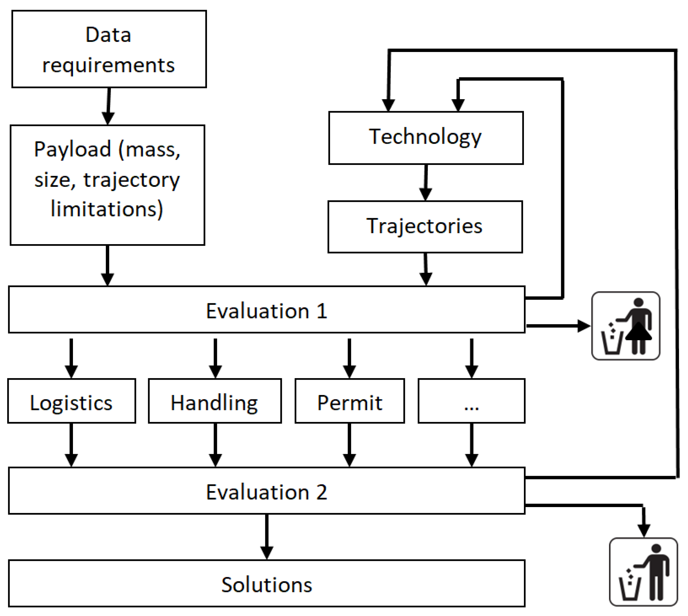
2.2.1. Solution Space and Concept Selection

At the beginning of the project, requirements for measurements and different basic ideas for the sensor carrier were collected openly. Within the research project, the methodology visualized in Figure 5 has been developed and was considered throughout the development.

Its general structure consists of an inner and an outer loop to reconsider solutions in another iteration after checking the requirements. The inner loop focuses on the pure technical feasibility to achieve the mission goals, whereas the outer loop additionally considers constraints such as handling, logistics, permission, and yet unknown constraints. The methodology has been applied to the initial technical solution space for the measurement platforms listed below.

Technical solution space

As a result of the first (inner) evaluation loop, the following solutions were compiled:

• Ascent technology
  Overarching technical possibilities to reach the altitude of 10 km; an ascent using aerostatic lift (balloon), ascending using its own propulsion, and a launch from a high altitude platform were considered.
• Trajectory type
  The UAS may drift with the wind or stay inside the dedicated airspace over the launch site.
• Propulsion type
  Possible options for the UAS, rocket, jet, and propellers powered by a gas- or electric engine, as well as systems without engines, have been identified.
• Platform type
  Options for the platform, rotary wing, fixed-wing, airship, and steerable bodies (e.g., rocket) have been considered.

In the first iteration, the use of gas-/jet-, and rocket engines have been excluded for environmental and handling reasons. In addition, the concept of a HAPS (high altitude platform system) has been put aside because of the feasibility during the project. Such HAPS weights are usually more than 25 kg, and, therefore, require certification and intense efforts to be implemented in the airspace.

Regarding airspace regulations and safety, the concept of an ascent with a balloon was denied, as drifting with the wind excludes the ability to stay within a certain operational volume. In addition to the current technology status regarding the weight of a sensing UAS system, the option to launch the UAS with a balloon and touchdown at another location within the wind drift direction would become interesting in the near future, depending on developments on the sensor packages and UAS technology/its weight.

Subsequently, electrically propelled ascents inside a dedicated operational volume denote the solution subspace.

The remaining concepts of an airship, a fixed-wing UAS, and a rotary wing can now be analyzed further. Considering the energy needed to fly against high wind speeds, airship and rotary wings have major drawbacks in comparison with a fixed-wing UAS. An airship with its volume needed for aerostatic lift faces enormous drag and, therefore, energy. A rotary wing consumes a minimal amount of energy at level flight at low velocities, but increased energy is needed to fly against high wind speed compared to a fixed wing, which itself needs to move forward with respect to the air mass to stay airborne.

As rotary-wing systems have the advantage of easy handling and not requiring special infrastructure for takeoff and landing, they were considered further. The dimension of the disadvantage of increased energy consumption of rotary-wing systems compared with fixed-wing aircraft during the climb, especially in high wind conditions, is assessed with simplified energy calculations. A mass of 5 kg has been chosen for these calculations. Assuming the required energy to climb per height element $E_{\delta H}$ (the derivative of the climb energy with respect to height) is

$$E_{\delta H}=P_{ideal}/w$$

(4)

with the ideal power $P_{ideal}$ and vertical climb speed w, the thrust vector has to be found to calculate the ideal power for the flight state during the climb using the equilibrium of forces

$${\overrightarrow{F}}_{Thrust}+{\overrightarrow{F}}_{Weight}+{\overrightarrow{F}}_{Drag}+{\overrightarrow{F}}_{Lift}=0$$

(5)

whereas the lift force generated by the wing is not present for rotary-wing systems. The aerodynamic forces are

$$F_{Drag,Lift}=p_{dynamic}·C_{Drag,Lift}·A_{Reference}$$

(6)

with $p_{dynamic}=0.5·\rho ·v^2$. For the calculation of a rotary wing, the assumed exemplary invariant body drag coefficient is $C_{Drag}=0.5$ according to the drag coefficient of a sphere in addition with a reference area of $A_{Body}=0.05$ m${}^2$. For the energy estimation of the fixed wing system, the approximation $C_{Drag}=C_{Drag0}+k·{C_{Lift}}^2$[38] is used, with an estimated drag coefficient at zero lift $C_{Drag0}=0.04$ and

$$k=\frac{1}{e·AR·\pi }$$

(7)

where e denotes the Oswald efficiency factor and $AR$ denotes the aspect ratio of the wing. For the calculations, $e=0.5$ and $AR=5$ are used in addition to a wing area of 0.5 m${}^2$. The ideal power (neglecting the profile drag of the propeller/rotary-wing blades) is calculated using momentum theory (according to e.g., [39]) and applied to the rotary wing as well as the propeller of the fixed wing system, assuming a radius of 0.4 m for both.

For the comparison between a rotary wing and a fixed-wing system, the wind speed (assumed to equal the horizontal true airspeed component) is varied from 0 km h${}^{-1}$ to 160 km h${}^{-1}$, and climb rates of $w=[10,20,40]$ m s${}^{-1}$ are assessed. The resulting energy consumption per unit height is shown in Figure 6 at an altitude of 5 km and an efficiency of $\eta =1$. Applying realistic efficiencies (e.g., overall efficiency of a power train including the propeller of $\eta =0.5$) will linearly increase the energy consumption.

As seen in Figure 6, the illustrative fixed-wing system is generally more efficient than the rotary-wing system for the specific mission and wind speeds up to 160 km h${}^{-1}$, except at a low wind speed of around 20 km h${}^{-1}$. For the parameters chosen, a climb speed of 20 m s${}^{-1}$ is optimal from an energy perspective, but will result in a high power requirement, which in turn leads to the increased mass of the propulsion system, possibly mismatching with the assumption of a total mass of 5 kg. Regarding rotary-wing systems and keeping in mind the exclusion of efficiency effects, a major disadvantage of rotary-wing systems is the need of additional energy during the descent for controlling the flight-except autorotation techniques, during which in turn an insufficient glide ratio is achieved (around 1:3 for a manned helicopter [40]).

However, even if it may be possible to reach an altitude of 10 km with copters, they have strong limitations for operation under high wind speed and it would barely be possible to meet the requirement of wind speed up to 100 km h${}^{-1}$. Such horizontal airspeed during an ascent up to 10 km altitude can up to now only be achieved by specifically designed fixed-wing aircraft. Therefore, the most flexible and promising solution was an ascending fixed-wing UAS, electrically propelled on its own on spiral trajectories to the designated altitude, which then descended again.

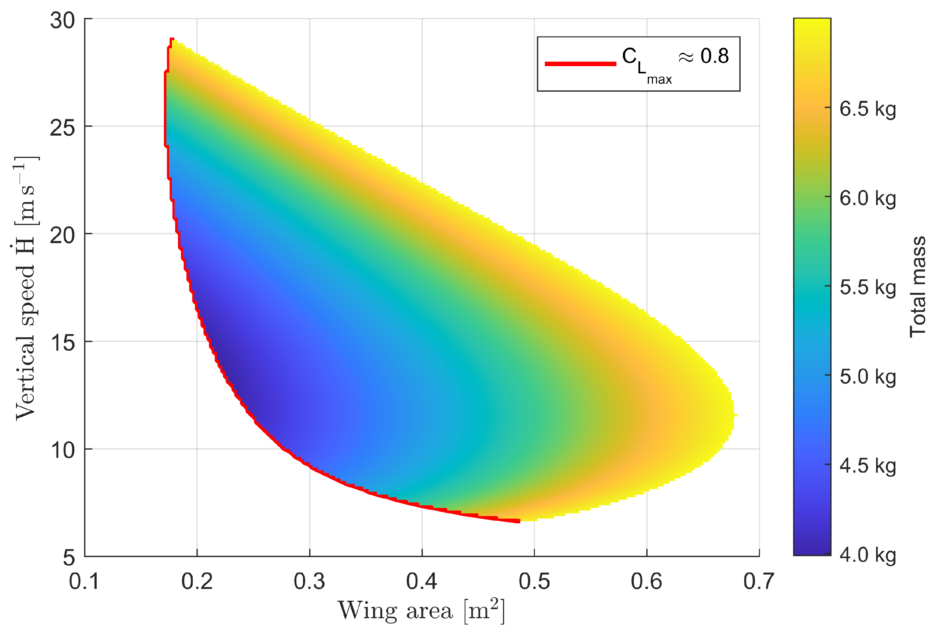
2.2.2. Parametric Design Approach

The technical feasibility of a fixed-wing UAS to meet the trajectory requirements is not questionable. Scaling up the measurement system will ease reaching the target altitude, but is in contrast to the challenge to design a small and lightweight system. A small system implies low cost and limited effort in obtaining permission. Starting from the trajectory requirements and boundary conditions (ascent up to 10 km with a horizontal airspeed component of 100 km h${}^{-1}$), the resulting total mass of the UAS shall be approximated by varying over two principal design parameters wing area and climb speed during the mission. Although the optimal climb speed during the mission might vary depending on the altitude, it is assumed as constant for the parametric design approach. In addition, the efficiency of the aircraft represented by $C_{Drag}=f\left(C_{Lift}\right)$, the efficiency of the power train as well as the efficiency of the propeller were approximated as constant over the mission. Hence, the Reynolds number effects are excluded. This vagueness has to be kept in mind during the interpretation of the results of the parametric design approach, as the propeller efficiency might vary up to 15% during the mission caused by a significant change of the Reynolds number with height [41]-not compensated by the increased rotational speed of the propeller needed to generate propulsion at lower air densities.

In the following, m denotes mass, H—height, and $\dot{H}$ its derivative with respect to time, A is the area, P—power, E—energy, F—force, C— coefficient, and p—pressure. As the total mass strongly depends on vertical speed $\dot{H}$ and wing area $A_{Wing}$, the basic equation is

$$m_{Total}=f(\dot{H},A_{Wing})$$

(8)

as an initial iteration. Subsequently, the function has to be framed further. $m_{total}$ can be split into four parts:

• $m_{Payload}$-the payload weight is assumed to be a fixed value;
• $m_{Airframe}$-the airframe weight can be considered to be proportional to the total mass;
• $m_{Motor}$-the motor mass can be estimated as a function of maximum continuous shaft power;
• $m_{Battery}$-and the battery mass depends on the energy needs including some overhead.

Therefore, the following dependencies are valid:

$$\begin{array}{cc}\hfill m_{Motor}& =f\left(P_{Moto{r}_{MAX}}\right)\hfill \\ \hfill m_{Battery}& =f\left(E_{Battery}\right)\hfill \end{array}$$

Assuming a constant horizontal velocity component in the wind fixed coordinate system as defined in the requirements, the remaining equations depending on variables are

$$\begin{array}{cc}\hfill E_{Battery}& =f(P_{Motor},\dot{H})\hfill \\ \hfill P_{Motor}& =f(F_{Thrust})\hfill \\ \hfill F_{Thrust}& =f(F_{Gravity},\dot{H},F_{Drag})\hfill \\ \hfill F_{Gravity}& =f(m_{Total})\hfill \\ \hfill F_{Drag}& =f(p_{dynamic},C_{Drag},A_{Wing})\hfill \\ \hfill p_{dynamic}& =f(H,\dot{H})\hfill \\ \hfill C_{Drag}& =f(C_{Lift})\hfill \\ \hfill C_{Lift}& =f(p_{dynamic},F_{Gravity},A_{Wing},\dot{H})\hfill \end{array}$$

which are either known or have to be approximated. Note that fixed requirements (e.g., horizontal airspeed, ceiling) do not show up in the illustrating functions and $V_{TrueAirspeed}$ has been substituted using $\dot{H}=f(V_{TrueAirspeed},V_{Horizontal})$.

For a payload of 0.5 kg, a horizontal airspeed $V_{Horizontal}$ of 100 km h${}^{-1}$, and an airframe to total mass ratio of 0.3, as well as an energy buffer of 30%, the calculations lead to the results shown in Figure 7. During the calculation, a limit for the dimensionless maximum lift generation coefficient $C_{L_{max}}$ has to be applied. The value of $C_{L_{max}}$ = 0.8 has been chosen but might be reassessed, as the value strongly depends on the aircraft design [42,43], such as airfoil selection, Reynolds number regime during flight, surface roughness and, hence, additionally, the effect of rain and icing on the airplane.

Figure 7 gives some important insights into the resulting design. The minimum in the mass is reached for small wing areas, and as mass is decreasing less than the wing area towards the left side of the calculated field, the wing loading increases toward small wing areas. Subsequently, this yields to the high overall lift coefficient, which has to be considered during the aircraft design, also characterized by the boundary of the resulting field. The mass minimum depending on vertical speed indicates a distinct minimal mass around 12 m s${}^{-1}$ with a gradient increasing towards higher wing areas. The field is only limited by the maximum total mass (criterion $m_{Total}<7$ kg, upper and right boundary) and the maximum overall lift coefficient ($C_{L_{max}}<0.8$, lower and left boundary.

In addition, the optimal vertical speed of approximately 12.5 m s${}^{-1}$ is relatively high for any wing area considering an average climb rate of airliners around 10 m s${}^{-1}$.

The results of such a parametric design have to be refined considering available components and physical constraints. In the project AEROMET_UAV, the refinements consisted of using the momentum theory (Froude and Rankine) [44] instead of a simple energy-efficiency approach and variations in the selected drive train components as well as further variations in trajectory parameters such as vertical and horizontal speed.

3. Results

3.1. Air and Ground Segment of the UAS

The developed UAS and its different subsystems as well as the strategy to mitigate the risk of In-Flight Icing are discussed subsequently. Figure 8 shows the final developed system on the catapult launcher. The positions of the meteorological sensor package and the sensor bay in the wing are marked up in the figure and discussed in the following.

3.1.1. Strategy to Mitigate the Risk of In-Flight Icing

As indicated before, in-flight icing has the potential to disrupt regular measurements with UAS, mostly depending on the mission and the site where the UAS is deployed. UAS flying mostly horizontally and, therefore, without the capabilities of climbing out of the icing zone are especially prone to in-flight icing. In addition to icing zones in cumulonimbus clouds, which can be actively avoided as their life cycle is temporally limited, the vertical extent of the icing zone within stratiform clouds (consisting of supercooled liquid water droplets) usually does not exceed 1 km (e.g., measurements in [45]). Currently, the key challenge for regular drone operations is icing detection, as indicated by Hann and Johansen [46]: “Ice detection is a key element for unmanned aircraft that are operating BVLOS and for systems with all-weather capabilities”. In addition, active in-flight de-icing techniques and (passive) anti-ice chemicals and coatings were considered for the mission of LUCA. As active de-icing relies on a substantial amount of electrical energy [47] and the active spray of chemicals during the flight inherits additional technical complications, icephobic coatings were considered during the design of the UAS LUCA, but the technology has not yet been accessible outside laboratories [46].

The operation of LUCA in icing conditions, therefore, relies on the current state, such as a mitigation-using forecast, e.g., ADWICE (Advanced Diagnosis and Warning System for Aircraft Icing Environments [48]). Although the forecast of icing is generally difficult, as the presence of supercooled liquid water strongly depends on aerosols and their properties [49], progress has been made in generating now-casts using remote sensing instruments [50,51,52]. On the other hand, the risk mitigation relies on the detection of in-flight icing. Therefore, a dedicated ice detection sensor has been developed and tested in the icing wind tunnel at the Technische Universität Braunschweig (Germany) in collaboration with the company Coldsense (Germany). However, the icing sensors have not yet been implemented and tested under real-world icing conditions up to now. During the flights performed so far, the strategy to detect icing consisted of an additional onboard “watchdog” to detect icing through performance degradation similar to [53]. In the Antarctic, rime ice is expected due to the low temperatures, and because “Rime ice shapes typically have a streamlined form with limited effect on the airfoil aerodynamics except for cases with extensive icing durations” [46], the UAS LUCA is expected to be capable of climbing through the icing zone [54] with its climb speed similar to an airliner climb. The mass increase is expected to be low, as liquid water content usually decreases with temperature and diminishes statistically below −10 °C [55]. In northern Germany, the expected mixed-ice accumulation denotes a threat to the aerodynamics of the UAS LUCA, and if this kind of icing is to be expected, regular flights have to be suspended or canceled based on the forecast/now-cast to mitigate the risk. Therefore, the developed strategy to mitigate the risk of in-flight icing consists of

• Situational awareness through the consultation of the forecast, in particular, the explicit forecast and now-cast of icing, humidity, liquid water content, and the presence of clouds.
• Detection of in-flight icing by using the onboard ice detection sensor and checking the consistency of performance data in combination with the probability of icing occurrence.
• Operational Procedures defined in the concept of operations based on a decision tree, to either climb through the icing zone, return to launch and recover the aircraft, or delay/cancel the operation prior to the UAS launch.

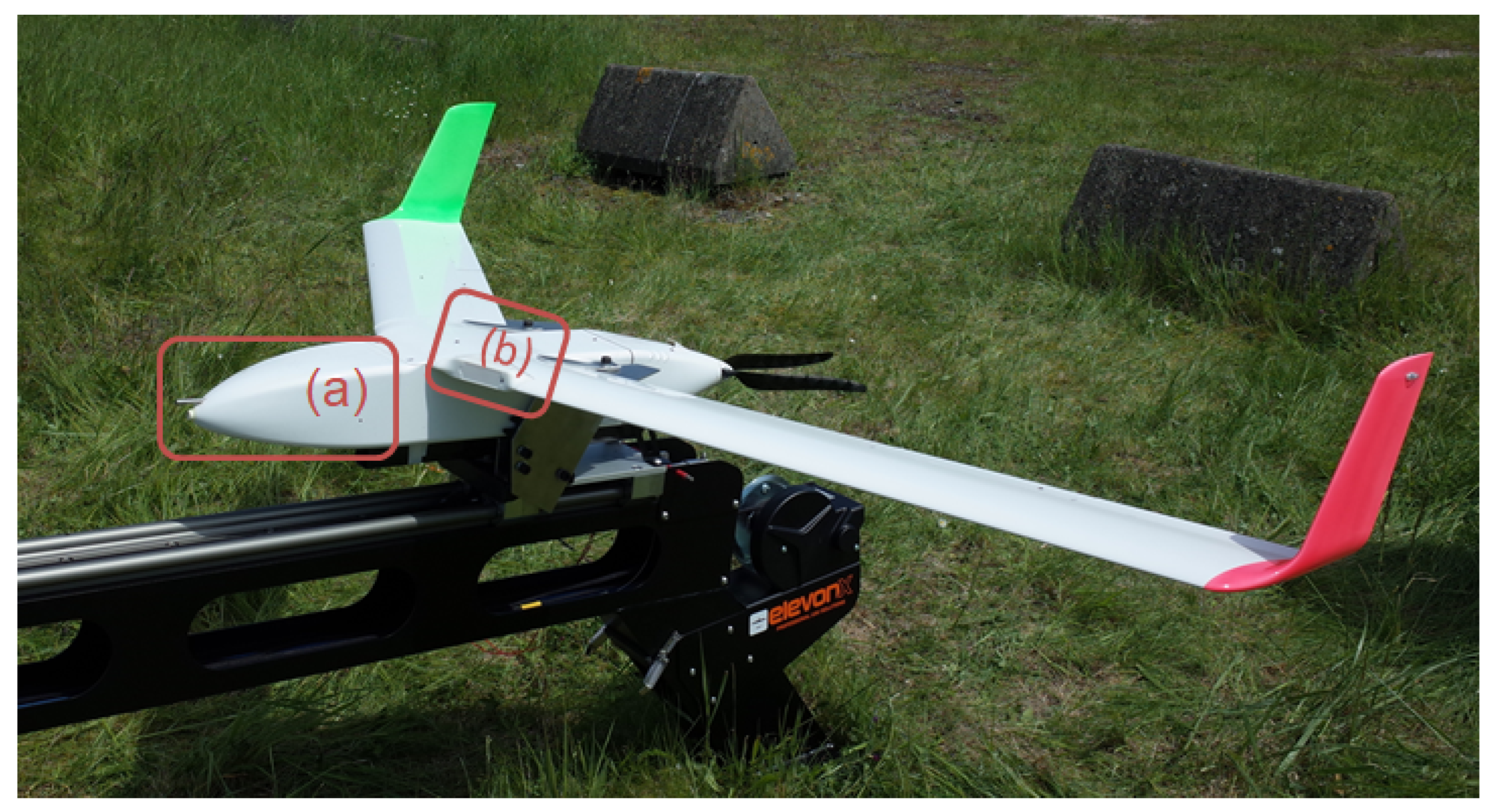
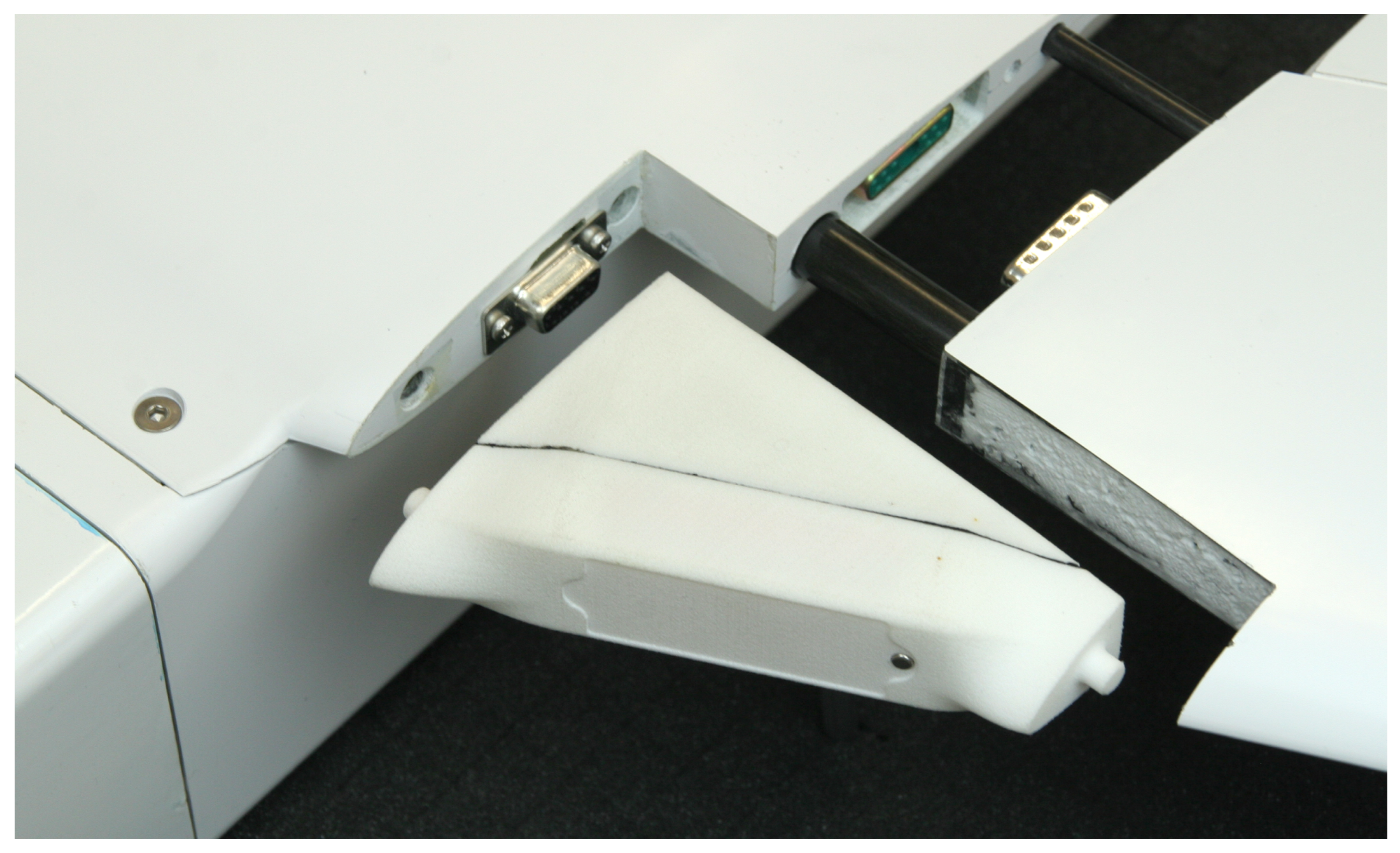
Currently, only the first point of the strategy has been applied during the flights, and more testing is required in the future.

3.1.2. Air Segment

LUCA is designed as a tailless aircraft with an electrically driven pusher propeller. The tailless configuration with a wingspan of 1.75 m results from reflections of minimizing the system components and keeping the propeller distant from the sensor package. The autopilot system for flight control consists of the commercially available hardware “Cube Orange” (HexAero, Singapore) based on the open hardware design “FMUv5” running the open source hardware “ArduPlane 4.1”. As the command and control link (C2), a 868 MHz long-range model RFD868x (RFDesign, Australia) is used as the primary link, and a commercially available RC-Module “Archer RS” (FrSky Electronic Co., Jiangsu, China) using a 2.4 GHz band as the secondary link. LUCA has three servos per wing which are responsible for flight control. For primary flight control (pitch and roll) the wing flaps (elevons) are redundant. This allows one actuator on each side to fail without affecting the flight control. The flaps and air brakes do not have a primary flight control function and cannot endanger the primary control due to their generated flight mechanical moment. The use is only intended for manual landing. The UAS is equipped with an ADS-B (automatic dependent surveillance–broadcast) receiver that registers position data from other nearby aircraft. The device is capable of detecting equipped aircraft within 150 km ADS-B and transmitting this information to the ground control station (GCS) to enable the controller to take evasive action.

Sensor package: The choice of sensors for the system test flights consisted of the humidity and temperature sensor HMP110 (Vaisala, Vantaa, Finland). For deriving the wind speed and wind direction, a miniaturized pitot tube was included in the measurement compartment providing measurements of the total pressure and dedicated positions around the airframe, pressure ports to measure static pressure. The difference between these pressure ports is the dynamic pressure, which provides information on the airflow. The integrated navigation solution of the autopilot system, which fuses measurements of the global navigation satellite system and measurements of the inertial measurement unit into position and attitude, was used to calculate the wind speed and wind direction according to [28].

Sensor bay in the wing: At the leading edge of the wing root, the system provides additional space for mission-specific sensor technology on either side of the fuselage. Form-fitting sensor units can easily be inserted in the resulting sensor bay. They are securely held in place when the wings are mounted to the fuselage. A configurable D-sub connector provides power, a data link, and optional pneumatic connections. Figure 9 shows the sensor bay and a custom-built ice detector unit (Coldsense Technologies, Braunschweig, Germany).

Aerial camera unit: A form-fitting aerial camera unit was developed to capture video and audio during the mission. It can be inserted in the previously described sensor bay. The inbuilt camera is capable of recording high-definition video at 60 frames per second, a small microphone captures an audio signal. In addition to scientific evaluation, the video recordings can provide valuable information for post-flight analysis of the mission regarding flight dynamics and control. A sample image of the aerial camera unit is shown in Figure 10.

3.1.3. Ground Control Station

The developed ground control station consists of a computer running the open source ground control station software “MissionPlanner” and a long-range radio frequency (868 MHz) modem including antennas. As a secondary link, telemetry data are transmitted to a handheld remote control station on 2.4 GHz which also bears the chance to intervene manually during the flight or even land the aircraft in the manual mode.

3.1.4. Launch and Landing Concept

Catapult launcher: For ensuring a controllable flight during the propeller run-up right after the launch, a minimum speed of 75 km h${}^{-1}$ is required due to the wing loading of 16 kg m${}^{-1}$. This can be accomplished by the spring-loaded catapult shown in Figure 8 (ElevonX, Tržič, Slovenia). A specially designed fixture to accommodate the aircraft on the catapult was later developed and integrated based on the first tests. Its total length of approximately 4 m and a folding mechanism make the catapult easy to transport. However, achieving the required minimum speed on such a short length while keeping the peak acceleration moderate is challenging. During initial testing, the velocity of the aircraft was determined by evaluating the individual frames of a high-speed camera located next to the catapult. The distance traveled from frame to frame times the frame rate of the camera yielded the velocity. The acceleration profile during the launch was recorded by the inbuilt inertial measurement unit (IMU). A test launch performed with an aircraft mass of 5.5 kg gave a final velocity of 75 km h${}^{-1}$ and a peak acceleration of about 10 g (10 times the Earth acceleration), which has to be considered during the design of the structure. For comparison, a catapult launcher for manned aircraft typically accelerates with less than 4 g.

Net landing: The high wing loading of the aircraft and a stall speed of around 65 km h${}^{-1}$ comparable to the minimum airspeed of a manned sailplane make a conventional landing challenging even in good visibility conditions. As visibility during night and in high wind speed conditions at Neumayer is low, an automatic landing has been implemented. Regarding the efforts needed to ensure conventional autonomous landings (e.g., a rangefinder applicable during rain and snowfall) and the risk of damage or even a complete loss of the system including its sensors, a landing into a net has been developed. Assuming changing wind directions and a horizontal position accuracy exceeding the vertical position accuracy, a landing into a horizontally oriented net as depicted in Figure 11 was opted for. The components of the net and materials have been chosen carefully so that the net can withstand even harsh environmental conditions such as Antarctic temperatures, high wind speed, ice, and snow. A specially developed automated flight maneuver ensures a safe landing after every mission. The final approach is oriented against the wind and targeted to a point a few meters above the net. When this point is reached, the aircraft will pitch down and dive right into the net where it can easily be recovered by the operating personnel. As the sensor package is implemented in a closed path, it is ensured that the sensors are not damaged.

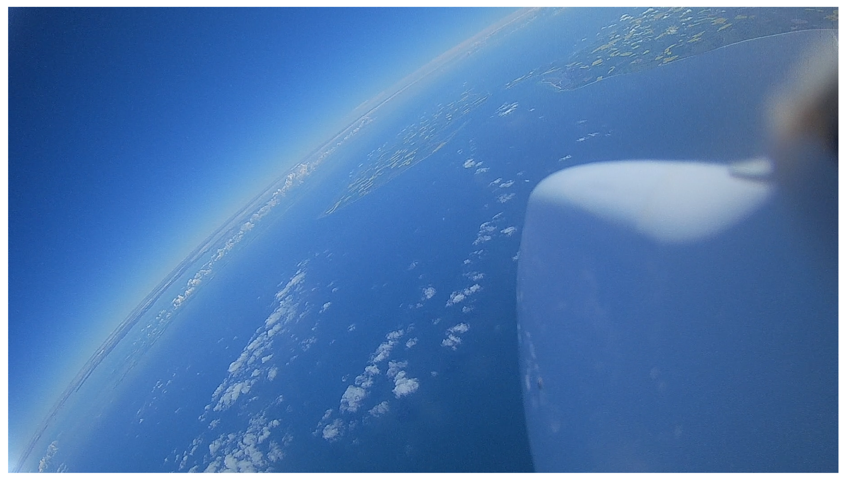
3.2. Flight Tests and First Measurements

To conduct flight tests, the permission needed for the planned mission and test site have to be granted by authorities. The requirements concerning safety and redundancy increase strongly with the weight of the UAS, and increase for air space that is not specifically reserved for the mission. The process to obtain permission to fly above an altitude of 120 m is significantly more demanding. For the performance flight tests with the newly developed system LUCA up to 10 km altitude, an explicit risk assessment according to the Specific Operations Risk Assessment (SORA) has been required by legislation from the European Union since 2021. The SORA process according to the EASA (European Union Aviation Safety Agency) ruleset implemented in Germany follows closely the proposals of JARUS (Joint Authorities for Rulemaking on Unmanned Systems), and might, therefore, be applied to other regions. As the operational volume for the mission was completely contained in a restricted airspace and over a controlled ground area, moderate requirements of the UAS, the operations, and the staff involved had to be met. Nevertheless, flight tests had to be announced early to the German Federal Agency for Air Traffic Control (BAF) and a NOTAM (notice to airmen) was published.

The performance flight tests were conducted in cooperation with the German Armed Forces in a reserved airspace over a controlled ground area at the coast of the Baltic See in the military restricted area of Todendorf (Panker), Schleswig–Holstein, in the north of Germany at the Baltic Sea, as shown in Figure 12.

After initial flight tests on nearby test sites and areas for recreational model aircraft flying, tests of the automated catapult launch, and tuning of the autopilot controller, efforts have been taken to test the automated net landing procedures, as missing the net would certainly destroy the UAS. The test for timing and positioning accuracy revealed the applicability of the landing maneuver, and maneuver tests distant from the ground provided insightful data to adjust the net landing maneuver trajectory. Several subsequent automated landings into the net finalized the successful development. The landing maneuver into the horizontal net as discussed above is shown in Figure 11. Due to the complexity of the system, basic flight tests, catapult launch tests and landing maneuver tests (including recurring tests after improvements of the UAS) started in 2019 and lasted until the flight tests up to higher altitudes were successful in October 2021. The maximum altitude flight tests were conducted between July 2020 and October 2021 during short campaigns in Todendorf (Panker), Germany. For validation of the first measurements and to retrieve environmental conditions, a radiosonde was launched in parallel to the flights of the UAS, and the first results are shown in [57]. An overview of the scale of the uncertainties based on simple RMSE (root mean square error) calculus between LUCA and the radiosonde data for two flight tests is shown in

Table 3. Uncertainty (RMSE) of the measurements based on the intercomparison between the UAS LUCA and a radiosonde for two test flights.

Date/Time	Pressure	Temperature	Dew Point	Wind FF	Wind DD
25 October 2021 09:41	0.5 hPa	1 K	4.8 K	2.7 m s${}^{-1}$	5°
26 October 2021 08:45	1.7 hPa	2.6 K	3.9 K	2.2 m s${}^{-1}$	7.6°

. Data uncertainty does not comply with the OSCAR “breakthrough” requirements as shown in Table 1, caused by the simplistic sensor package and sensor integration as well as the spatiotemporal dislocation between the radiosonde and the UAS during the intercomparison.

The trajectory of the flight tests consists of a climb into the direction of the center of the segregated airspace and subsequent spiral pattern in a cylinder of less than 1 km diameter up to the ceiling altitude. In order not to leave the cylinder even under high wind speed conditions, the horizontal component of the airspeed is 100 km h${}^{-1}$. The vertical speed for climb and descent during the flight tests was between 10 m s${}^{-1}$ and 15 m s${}^{-1}$. The descent is organized similarly but with the propeller in the windmilling state to blast the trajectory energy and protect the UAS from exceeding the maximum speed (never exceeding the speed) $V_{NE}$ = 240 km h${}^{-1}$. The performance parameters of LUCA and onboard data as well as ADS-B data are constantly monitored by the ground crew and any faults are passed on to the remote pilot. The ground crew can initiate a return-to-launch maneuver at any time through either the 2.4 GHz or the 868 MHz radio link. The remote pilot can take over manual control of LUCA as soon as LUCA is within visual line of sight control. Both radio links were reliable even for a distance beyond 10 km, despite short connection losses depending on the attitude of the UAS with respect to the ground segment antennas. As the flight tests were conducted in restricted airspace, no air traffic was encountered during the operation of LUCA.

During the flight tests with the system originally designed for flights in the Antarctic (cold conditions), the power electronics of the drive train overheated under summer-like mid-European conditions. The mitigating action that has been taken in the field was to implement several circular holding patterns at constant altitudes to facilitate the cooling down of the electronics. The performance flight tests conducted during the campaigns in Todendorf (Panker), Germany, are listed in

Table 4. Table of the envelope flight tests in the military restricted area Todendorf (Panker). The number of flights is limited as the clearance for takeoff depended on coincident military training activities.

Date and Time	Altitude Reached	Wind Speed (Maximum)	Temperature (Minimum)
03 July 2020 08:11	3.3 km	55 km h${}^{-1}$	−4 °C
28 May 2021 09:24	4.6 km	60 km h${}^{-1}$	−20 °C
28 September 2021 13:24	7.9 km	60 km h${}^{-1}$	−35 °C
25 October 2021 09:41	3.8 km	65 km h${}^{-1}$	−8 °C
25 October 2021 12:34	8.8 km	100 km h${}^{-1}$	−45 °C
26 October 2021 08:45	10.0 km	90 km h${}^{-1}$	−50 °C
28 October 2021 07:20	9.9 km	60 km h${}^{-1}$	−47 °C
28 October 2021 13:07	8.8 km	80 km h${}^{-1}$	−38 °C
29 October 2021 07:22	8.9 km	85 km h${}^{-1}$	−42 °C

. LUCA and radiosonde data are partly available at [58,59].

The table focuses on altitude, wind speed, and temperature. The envelope flight tests for maximum airspeed at sea level reached a speed of 240 km h${}^{-1}$ during horizontal flight segments. The maximum altitude was limited at the beginning by power electronic overheating but increased with time until October 2021, when the design altitude was reached. The encountered environmental conditions comprised up to 100 km h${}^{-1}$ wind speed, which designates the design wind speed, and a minimum air temperature of −50 °C, which is significantly higher than the minimum temperature considered for the design with −80 °C (Antarctic atmospheric conditions). Icing has neither been detected nor encountered during the flight, and as the ADWICE forecast showed a negligible risk of icing during the flight tests, the ice detector unit in the wing’s sensor bay was replaced by the aerial camera unit to record insightful videos. Extensive tests in icing conditions to evaluate the risk mitigation strategy have to be performed in the future to assess the flight envelope in icing conditions.

4. Discussion and Conclusions

In this study, a technical approach to designing and deploying drones for atmospheric soundings similar to commercial aircraft-based observations, radiosondes, and dropsondes is shown.

The upper air in situ data for numerical weather predictions and climate monitoring are weather balloon data. From the perspectives of NWP and researchers conducting local measurement campaigns, drone-based atmospheric soundings bear the chance of additional observations of the atmosphere in an environmentally friendly and cost-effective way. As drone-based observations may provide data in the planetary boundary layer, which undergoes changes in short time scales, and less frequent observations above the troposphere might be sufficient, opting for the thinning out of the frequency of radiosonde ascents will further increase the benefits of UAS observations to costs and the environment.

Herein, we present a methodology to develop such systems based on requirements defined previously for the application area. A comparison between the requirements for measurements in northern Germany and the northern coast of Antarctica reveals large differences in temperature, wind speed distribution with height, visibility, and the risk of icing. For the region of central Europe, there is currently one UAS system based on multi-copters deployed for additional atmospheric soundings to be used in operational NWP [12]. Applying the developed methodology for the combination of the assessed challenges for Europe and Antarctica, it was found that a fixed-wing UAS will fulfill the requirements best. A parametric design approach has then been applied using the estimated functions of basic energy/power/efficiency relations. The resulting field of the air segment’s total mass over the vertical ascent speed and wing area was subsequently used to design the UAS.

As the developed UAS, which is a fixed-wing small UAS representing the MASE (medium altitude, short endurance) class [60], is intended to be used in low visibility conditions and during the night, automated launch and recovery systems have been developed. While the automated launch consists of a spring-loaded catapult, the “splashdown”-concept is set up as a vertical dive into a horizontal net, where the UAS is supposed to rest until it is retrieved by the operational staff.

Permission to fly up to 10 km was granted in a restricted area, where both the air- and the ground risk are low since both airspace and ground are under military control. The UAS was successfully tested within its design envelope and sounded the atmosphere up to 10 km in a wind speed reaching 100 km h${}^{-1}$.

The need for improvements has been found regarding the stability of the communication and control link of the UAS, which could be addressed by using a different frequency band and higher transmission power for which it is required to apply for. Weakness of the system was also found regarding the thermal management of the electrical power train for the environmental conditions in Europe during the summer. Resolving the issue with better cooling would implicate cold temperatures of the electronics during operations in Antarctica, which potentially reaches down beyond the lower certification level of the electronics.

The conducted flight performance tests can be used to refine the analytical expressions, e.g., $C_D=f\left(C_L\right)$ or the power train efficiency, which will be reflected in more detailed parametric design parameters in the future, and enable the improved design of a UAS for predefined requirements. During the performance test phase, the atmospheric measurements were performed with low-quality sensors, as the risk of harming sophisticated sensors had to be reduced. A more adequate sensor package has to be mounted on the UAS, when measurements have priority over flight performance tests, e.g., for the upcoming WMO UAS Demonstration Campaign [61].

References

1. World Meteorological Organisation (WMO). GCOS, 171. The GCOS Reference Upper-Air Network (GRUAN): Guide; WMO: Geneva, Switzerland, 2013. [Google Scholar]
2. Durre, I.; Yin, X.; Vose, R.S.; Applequist, S.; Arnfield, J. Enhancing the Data Coverage in the Integrated Global Radiosonde Archive. J. Atmos. Ocean. Technol. 2018, 35, 1753–1770. [Google Scholar] [CrossRef]
3. NOAA-AMDAR. Available online: https://amdar.noaa.gov/ (accessed on 14 October 2022).
4. Jonassen, M.O.; Ólafsson, H.; Ágústsson, H.; Rögnvaldsson, Ó.; Reuder, J. Improving High-Resolution Numerical Weather Simulations by Assimilating Data from an Unmanned Aerial System. Mon. Weather Rev. 2012, 140, 3734–3756. [Google Scholar] [CrossRef] [Green Version]
5. Flagg, D.D.; Doyle, J.D.; Holt, T.R.; Tyndall, D.P.; Amerault, C.M.; Geiszler, D.; Haack, T.; Moskaitis, J.R.; Nachamkin, J.; Eleuterio, D.P. On the Impact of Unmanned Aerial System Observations on Numerical Weather Prediction in the Coastal Zone. Mon. Weather Rev. 2018, 146, 599–622. [Google Scholar] [CrossRef]
6. Rendón, A.M.; Salazar, J.F.; Palacio, C.A.; Wirth, V.; Brötz, B. Effects of Urbanization on the Temperature Inversion Breakup in a Mountain Valley with Implications for Air Quality. J. Appl. Meteorol. Climatol. 2014, 53, 840–858. [Google Scholar] [CrossRef]
7. Glojek, K.; Močnik, G.; Alas, H.D.C.; Cuesta-Mosquera, A.; Drinovec, L.; Gregorič, A.; Ogrin, M.; Weinhold, K.; Ježek, I.; Müller, T.; et al. The Impact of Temperature Inversions on Black Carbon and Particle Mass Concentrations in a Mountainous Area. Atmos. Chem. Phys. 2022, 22, 5577–5601. [Google Scholar] [CrossRef]
8. Sun, Q.; Vihma, T.; Jonassen, M.O.; Zhang, Z. Impact of Assimilation of Radiosonde and UAV Observations from the Southern Ocean in the Polar WRF Model. Adv. Atmos. Sci. 2020, 37, 441–454. [Google Scholar] [CrossRef] [Green Version]
9. Evans, M.; Knippertz, P.; Akpo, A.; Allan, R.P.; Amekudzi, L.; Brooks, B.; Chiu, J.C.; Coe, H.; Fink, A.H.; Flamant, C.; et al. Policy Findings from the DACCIWA Project; Technical Report; Zenodo: Geneva, Switzerland, 2018. [Google Scholar]
10. Bromwich, D.H.; Werner, K.; Casati, B.; Powers, J.G.; Gorodetskaya, I.V.; Massonnet, F.; Vitale, V.; Heinrich, V.J.; Liggett, D.; Arndt, S.; et al. The Year of Polar Prediction in the Southern Hemisphere (YOPP-SH). Bull. Am. Meteorol. Soc. 2020, 101, E1653–E1676. [Google Scholar] [CrossRef]
11. Pinto, J.O.; O’Sullivan, D.; Taylor, S.; Elston, J.; Baker, C.B.; Hotz, D.; Marshall, C.; Jacob, J.; Barfuss, K.; Piguet, B.; et al. The Status and Future of Small Uncrewed Aircraft Systems (UAS) in Operational Meteorology. Bull. Am. Meteorol. Soc. 2021, 102, E2121–E2136. [Google Scholar]
12. Leuenberger, D.; Haefele, A.; Omanovic, N.; Fengler, M.; Martucci, G.; Calpini, B.; Fuhrer, O.; Rossa, A. Improving High-Impact Numerical Weather Prediction with Lidar and Drone Observations. Bull. Am. Meteorol. Soc. 2020, 101, E1036–E1051. [Google Scholar] [CrossRef] [Green Version]
13. All-Weather Drone. Available online: https://projekte.ffg.at/projekt/4119066 (accessed on 6 October 2022).
14. Kräuchi, A.; Philipona, R. Return Glider Radiosonde for in Situ Upper-Air Research Measurements. Atmos. Meas. Tech. 2016, 9, 2535–2544. [Google Scholar] [CrossRef] [Green Version]
15. Schuyler, T.J.; Gohari, S.M.I.; Pundsack, G.; Berchoff, D.; Guzman, M.I. Using a Balloon-Launched Unmanned Glider to Validate Real-Time WRF Modeling. Sensors 2019, 19, 1914. [Google Scholar] [CrossRef] [PubMed]
16. Secretariat of the Antarctic Treaty. Compilation of Key Documents of the Antarctic Treaty, 4th ed.; Secretariat of the Antarctic Treaty: Buenos Aires, Argentina, 2019. [Google Scholar]
17. Schmithüsen, H. Radiosonde Measurements from Neumayer Station (1983-02 et Seq). 2022. Available online: https://doi.pangaea.de/10.1594/PANGAEA.940584 (accessed on 3 September 2022).
18. Wetter Und Klima-Deutscher Wetterdienst-Our Services-Open Data Server. Available online: https://www.dwd.de/EN/ourservices/opendata/opendata.html (accessed on 6 October 2022).
19. WMO. AMDAR Reference Manual: Aircraft Meteorological Data Relay; Number 958 in WMO; Secretariat of the World Meteorological Organization: Geneva, Switzerland, 2003. [Google Scholar]
20. Wang, J.; Hock, T.; Cohn, S.A.; Martin, C.; Potts, N.; Reale, T.; Sun, B.; Tilley, F. Unprecedented Upper-Air Dropsonde Observations over Antarctica from the 2010 Concordiasi Experiment: Validation of Satellite-Retrieved Temperature Profiles. Geophys. Res. Lett. 2013, 40, 1231–1236. [Google Scholar] [CrossRef]
21. WMO. Global Observing System. Available online: https://public.wmo.int/en/programmes/global-observing-system (accessed on 16 July 2022).
22. WMO. Guide to Instruments and Methods of Observation, 2018th ed.; Number 8 in WMO; WMO: Geneva, Switzerland, 2018. [Google Scholar]
23. WMO. OSCAR-Observing Systems Capability Analysis and Review Tool; WMO: Geneva, Switzerland, 2015. [Google Scholar]
24. Bärfuss, K.; Pätzold, F.; Altstädter, B.; Kathe, E.; Nowak, S.; Bretschneider, L.; Bestmann, U.; Lampert, A. New Setup of the UAS ALADINA for Measuring Boundary Layer Properties, Atmospheric Particles and Solar Radiation. Atmosphere 2018, 9, 28. [Google Scholar] [CrossRef] [Green Version]
25. Majewski, J. The Dynamic Behaviour of Capacitive Humidity Sensors. Devices Methods Meas. 2020, 11, 53–59. [Google Scholar] [CrossRef]
26. Stickney, T.M.; Shedlov, M.W.; Thompson, D.I. Goodrich Total Temperature Sensors; Technical Report; Goodrich: Burnsville, MN, USA, 1994. [Google Scholar]
27. Wilson, T.C.; Brenner, J.; Morrison, Z.; Jacob, J.D.; Elbing, B.R. Wind Speed Statistics from a Small UAS and Its Sensitivity to Sensor Location. Atmosphere 2022, 13, 443. [Google Scholar] [CrossRef]
28. Rautenberg, A.; Graf, M.S.; Wildmann, N.; Platis, A.; Bange, J. Reviewing Wind Measurement Approaches for Fixed-Wing Unmanned Aircraft. Atmosphere 2018, 9, 422. [Google Scholar] [CrossRef] [Green Version]
29. Witte, B.M.; Singler, R.F.; Bailey, S.C.C. Development of an Unmanned Aerial Vehicle for the Measurement of Turbulence in the Atmospheric Boundary Layer. Atmosphere 2017, 8, 195. [Google Scholar] [CrossRef] [Green Version]
30. Alaoui-Sosse, S.; Durand, P.; Medina, P.; Pastor, P.; Lothon, M.; Cernov, I. OVLI-TA: An Unmanned Aerial System for Measuring Profiles and Turbulence in the Atmospheric Boundary Layer. Sensors 2019, 19, 581. [Google Scholar] [CrossRef] [Green Version]
31. Schmithüsen, H. Meteorological Synoptical Observations from Neumayer Station, 1981-01 to 2019-01, Reference List of 457 Datasets. Available online: https://doi.pangaea.de/10.1594/PANGAEA.911242 (accessed on 21 February 2022).
32. Sørensen, K.L.; Borup, K.T.; Hann, R.; Hansbø, M. UAV Atmospheric Icing Limitations, Climate Report for Norway and Surrounding Regions; Technical Report; UBIQ Aerospace: Trondheim, Norway, 2021. [Google Scholar]
33. Bernstein, B.C.; McDonough, F.; Politovich, M.K.; Brown, B.G.; Ratvasky, T.P.; Miller, D.R.; Wolff, C.A.; Cunning, G. Current Icing Potential: Algorithm Description and Comparison with Aircraft Observations. J. Appl. Meteorol. Climatol. 2005, 44, 969–986. [Google Scholar] [CrossRef]
34. EASA. Easy Access Rules for Unmanned Aircraft Systems (Regulation (EU) 2019/947 and Regulation (EU) 2019/945). Available online: https://www.easa.europa.eu/document-library/easy-access-rules/easy-access-rules-unmanned-aircraft-systems-regulation-eu (accessed on 7 February 2022).
35. JARUS 2021 Spring Virtual Plenary Meeting Information | JARUS. Available online: http://jarus-rpas.org/ (accessed on 14 October 2022).
36. Beaumont, N.J.; Aanesen, M.; Austen, M.C.; Börger, T.; Clark, J.R.; Cole, M.; Hooper, T.; Lindeque, P.K.; Pascoe, C.; Wyles, K.J. Global Ecological, Social and Economic Impacts of Marine Plastic. Mar. Pollut. Bull. 2019, 142, 189–195. [Google Scholar] [CrossRef]
37. Gallo, F.; Fossi, C.; Weber, R.; Santillo, D.; Sousa, J.; Ingram, I.; Nadal, A.; Romano, D. Marine Litter Plastics and Microplastics and Their Toxic Chemicals Components: The Need for Urgent Preventive Measures. Environ. Sci. Eur. 2018, 30, 13. [Google Scholar] [CrossRef] [PubMed]
38. Sun, J.; Hoekstra, J.M.; Ellerbroek, J. Aircraft Drag Polar Estimation Based on a Stochastic Hierarchical Model. In Proceedings of the Eighth SESAR Innovation Days, Salzburg, Austria, 3–7 December 2018. [Google Scholar]
39. van der Wall, B.G. Grundlagen der Hubschrauber-Aerodynamik, 1st ed.; VDI-Buch; Springer: Wiesbaden, Germany, 2015. [Google Scholar]
40. Lee, A.Y.; Bryson, A.E.; Hindson, W.S. Optimal Landing of a Helicopter in Autorotation. J. Guid. Control. Dyn. 1988, 11, 7–12. [Google Scholar] [CrossRef] [Green Version]
41. Merchant, M.; Miller, L.S. Propeller performance measurement for low Reynolds number UAV applications. In Proceedings of the 44th AIAA Aerospace Sciences Meeting and Exhibit, Reno, NV, USA, 9 January 2006–12 January 2006; American Institute of Aeronautics and Astronautics: Reston, VA, USA, 2006. [Google Scholar]
42. Schlichting, H.; Truckenbrodt, E. Aerodynamik des Flugzeuges: Zweiter Band: Aerodynamik des Tragflügels (Teil II), des Rumpfes, der Flügel-Rumpf-Anordnungen und der Leitwerke; Springer: Berlin/Heidelberg, Germany, 2013. [Google Scholar]
43. Sadraey, M. Design of Unmanned Aerial Systems; Wiley: Hoboken, NJ, USA, 2020. [Google Scholar]
44. Sforza, P.M. Theory of Aerospace Propulsion, 2nd ed.; Aerospace Engineering; Elsevier: Amsterdam, The Netherlands, 2017. [Google Scholar]
45. Bernstein, B.C.; Rasmussen, R.M.; McDonough, F.; Wolff, C. Keys to Differentiating between Small- and Large-Drop Icing Conditions in Continental Clouds. J. Appl. Meteorol. Climatol. 2019, 58, 1931–1953. [Google Scholar] [CrossRef]
46. Hann, R.; Johansen, T.A. Unsettled Topics in Unmanned Aerial Vehicle Icing; SAE Technical Paper EPR2020008; SAE International: Warrendale, PA, USA, 2020. [Google Scholar]
47. Hann, R.; Enache, A.; Nielsen, M.C.; Stovner, B.N.; van Beeck, J.; Johansen, T.A.; Borup, K.T. Experimental Heat Loads for Electrothermal Anti-Icing and De-Icing on UAVs. Aerospace 2021, 8, 83. [Google Scholar] [CrossRef]
48. Kalinka, F.; Roloff, K.; Tendel, J.; Hauf, T. The In-flight Icing Warning System ADWICE for European Airspace – Current Structure, Recent Improvements and Verification Results. Meteorol. Z. 2017, 4, 441–455. [Google Scholar] [CrossRef]
49. Petäjä, T.; Tabakova, K.; Manninen, A.; Ezhova, E.; O’Connor, E.; Moisseev, D.; Sinclair, V.A.; Backman, J.; Levula, J.; Luoma, K.; et al. Influence of Biogenic Emissions from Boreal Forests on Aerosol–Cloud Interactions. Nat. Geosci. 2022, 15, 42–47. [Google Scholar] [CrossRef]
50. Luke, E.P.; Kollias, P.; Shupe, M.D. Detection of Supercooled Liquid in Mixed-Phase Clouds Using Radar Doppler Spectra. J. Geophys. Res. Atmos. 2010, 115, D19. [Google Scholar] [CrossRef] [Green Version]
51. Bühl, J.; Seifert, P.; Myagkov, A.; Ansmann, A. Measuring Ice- and Liquid-Water Properties in Mixed-Phase Cloud Layers at the Leipzig Cloudnet Station. Atmos. Chem. Phys. 2016, 16, 10609–10620. [Google Scholar] [CrossRef] [Green Version]
52. Gaussiat, N.; Hogan, R.J.; Illingworth, A.J. Accurate Liquid Water Path Retrieval from Low-Cost Microwave Radiometers Using Additional Information from a Lidar Ceilometer and Operational Forecast Models. J. Atmos. Ocean. Technol. 2007, 24, 1562–1575. [Google Scholar] [CrossRef]
53. Rotondo, D.; Cristofaro, A.; Johansen, T.A.; Nejjari, F.; Puig, V. Robust Fault and Icing Diagnosis in Unmanned Aerial Vehicles Using LPV Interval Observers. Int. J. Robust Nonlinear Control 2019, 29, 5456–5480. [Google Scholar] [CrossRef]
54. Siquig, R. Impact of Icing on Unmanned Aerial Vehicle (UAV) Operations; Technical Report ADA231191; Naval Environmental Prediction Research: Facility Monterey, CA, USA, 1990. [Google Scholar]
55. Cober, S.G.; Isaac, G.A. Characterization of Aircraft Icing Environments with Supercooled Large Drops for Application to Commercial Aircraft Certification. J. Appl. Meteorol. Climatol. 2012, 51, 265–284. [Google Scholar] [CrossRef]
56. Open Flightmaps|Aeronautical Data under a Public License. Available online: https://www.openflightmaps.org/ (accessed on 14 October 2022).
57. Bärfuss, K.B.; Schmithüsen, H.; Lampert, A. Drone-Based Meteorological Observations up to the Tropopause. Atmos. Meas. Tech. Discuss. 2022, 2022, 1–26. [Google Scholar]
58. Bärfuss, K.; Schmithüsen, H.; Dirksen, R.; Bretschneider, L.; Pätzold, F.; Bollmann, S.; Wickboldt, H.; von Unwerth, M.; Asmussen, M.; Schwarting, T.; et al. Radiosonde Measurements Co-Located with Ascends of the Unmanned Aerial System LUCA (Panker, Germany 2020-07-03 and 2021-05-28), PANGAEA, 2021. Available online: https://doi.pangaea.de/10.1594/PANGAEA.937556 (accessed on 22 October 2022).
59. Bärfuss, K.; Schmithüsen, H.; Dirksen, R.; Bretschneider, L.; Pätzold, F.; Bollmann, S.; Wickboldt, H.; von Unwerth, M.; Asmussen, M.; Schwarting, T.; et al. Atmospheric Profile Measurements Conducted by the Unmanned Aerial System LUCA (Panker, Germany 2020-07-03 and 2021-05-28), PANGAEA, 2021. Available online: https://doi.pangaea.de/10.1594/PANGAEA.937555 (accessed on 22 October 2022).
60. Watts, A.C.; Ambrosia, V.G.; Hinkley, E.A. Unmanned Aircraft Systems in Remote Sensing and Scientific Research: Classification and Considerations of Use. Remote Sens. 2012, 4, 1671–1692. [Google Scholar] [CrossRef]
61. WMO. WMO UAS Demonstration Campaign Description|World Meteorological Organization. Available online: https://community.wmo.int/uas-demonstration/description (accessed on 16 February 2022).
Figure 1. Global coverage of vertical atmospheric in situ measurements and their densities (logarithm with the base of 10 as the number of stations within 500 km) on a world map (Lambert Azimuthal Equal-Area Projection). In panel (a), the data from the Integrated Global Radiosonde Archive (IGRA) Version 2 stations [2] are shown, revealing areas with low densities over the oceans. In panel (b), vertical profiles of AMDAR measurements are shown (source [3]), revealing low densities over the oceans and Asia, and generally in the southern hemisphere.
Drones 06 00404 g001
Figure 2. Cumulative probability function of wind speeds calculated of the observed conditions at the Lindenberg and Neumayer Station sites for the time period 2016–2018. The green lines represent Lindenberg (Germany), the blue lines Neumayer (Antarctica). The solid lines describe the wind speed probability close to the ground. The dashed lines denote the wind speed distribution at 8 km altitude. Evidence of jet streams are visible for Lindenberg, whereas the wind speed at Neumayer is relatively moderate at this altitude. The dotted lines represent the probability of the maximum wind speed at a time for the atmospheric column between 200 m AMSL up to 10 km AMSL. Again, higher wind speeds caused by jet streams are observed for the Lindenberg site. The gray lines (solid, dashed and dotted) denote design parameters of the UAS LUCA and are discussed in Section 3.1.2.
Drones 06 00404 g002
Figure 3. Cumulative wind probability of wind-induced environmental constraints as a function of wind speed at Neumayer Station III. Data shown here are 3-hourly synoptic observations for the decade 2012 to 2021 [31]. The blue line denotes the accumulated histogram of observed wind speed. The black lines show the probability of drifting (below eye level) and/or blowing snow (above eye level) as a function of wind speed. Similarly, red lines indicate the probability of visibility constraints in the observed categories.
Drones 06 00404 g003
Figure 4. Total acquisition cost for radiosonde and UAS-based soundings as a function of the number of flights. The potential reduction in acquisition cost is depicted by the red line, assuming a UAS may be used for 25 soundings.
Drones 06 00404 g004
Figure 5. Methodology to converge ideas into a feasible solution space. Subsequent to the generation of requirements, the solution space is iterated and sorted out by the first evaluation in a technical feasibility loop. The remaining solutions are then evaluated against soft and disruptive demands, such as logistics, handling, and permission. Since technology evolves and demands might change, the process has to be applied dynamically in time and solutions have to be reevaluated frequently for future potential UAS deployment.
Drones 06 00404 g005
Figure 6. Energy consumption per height unit for a rotary wing and a fixed-wing system for wind speed from 0 km h 1 to 160 km h 1 , which is assumed to equal the horizontal true airspeed component, and climb rates of w = [ 10 , 20 , 40 ] m s 1 . As a reference, the potential energy increase per height unit is shown. Thrust efficiency was neglected for the calculations, but might be applied as a linear coefficient on the results to calculate more realistic energy consumption.
Drones 06 00404 g006
Figure 7. Total UAS mass under the prerequisites of reaching 10 km with a horizontal airspeed of 100 km 1 . Additional assumptions are the payload mass of 0.5 kg, the energy buffer of 30%, and an airframe to total mass ratio of 0.3. The borders of the field are determined by limits set to C L < 0.8 and a total mass exceeding 7 kg during the calculations.
Drones 06 00404 g007
Figure 8. System LUCA on the catapult launcher during a test flight campaign in Todendorf (Panker), Germany on 28 May 2021. The locations of the meteorological sensor package (a) and the sensor bay in wing (b) are indicated.
Drones 06 00404 g008
Figure 9. Sensor bay included at the wing root on both sides of the fuselage. Additional sensors, e.g., an ice detector unit, can be inserted. The unit is securely held in place when the wings are fully mounted to the fuselage.
Drones 06 00404 g009
Figure 10. Photo taken by the aerial camera unit during a test flight from the military restricted area Todendorf (Panker), Germany, at an altitude of around 8000 m on 28 October 2021, with a view of the Baltic Sea, the island of Fehmarn, and the horizon of the Danish coastline.
Drones 06 00404 g010
Figure 11. The missions terminate with an automated landing into a horizontally oriented net. The time interval between the aircraft positions in this multi-exposure image is 1/6 s. After a horizontal approach including a decision phase, the main motor is stopped and the aircraft dives into the horizontal net with dimensions of 16 m × 16 m.
Drones 06 00404 g011
Figure 12. Map of the region where flight tests up to 10 km were conducted. The restricted areas ED-R10 (emphasized in light yellow) enveloped the operational volume, and the Baltic Sea below the airspace was secured by two military boats. The map center is at 54.5° N and 10.7° E. Map source [56].
Drones 06 00404 g012