Abstract
The development of UAV sensors has made it possible to obtain a diverse array of spectral images in a single flight. In this study, high-resolution UAV-derived images of urban areas were employed to create land cover maps, including car-road, sidewalk, and street vegetation. A total of nine orthoimages were produced, and the variables effective in producing UAV-based land cover maps were identified. Based on analyses of the object-based images, 126 variables were derived by computing 14 statistical values for each image. The random forest (RF) classifier was used to evaluate the priority of the 126 variables. This was followed by optimizing the RF through variable reduction and by comparing the initial and optimized RF, the utility of the high-priority variable was evaluated. Computing variable importance, the most influential variables were evaluated in the order of normalized digital surface model (nDSM), normalized difference vegetation index (NDVI), land surface temperature (LST), soil adjusted vegetation index (SAVI), blue, green, red, rededge. Finally, no significant changes between initial and optimized RF in the classification were observed from a series of analyses even though the reduced variables number was applied for the classification.
1. Introduction
Land cover maps are produced in line with specific classification systems based on the optical and physical conditions of the ground surface and serve as primary data for assessing the current status of an area. At the urban level, the maps are used as a scientific basis for city planning, including analyses of land aptitude, environmental assessments, and urban regeneration; whereas academically, they play an essential role in various studies, for instance thermal environment analyses, airflow simulations, and ecosystem surveys [1,2,3,4,5]. In the Republic of Korea, the national land cover maps are updated every 1–10 years, depending on the government’s budget allocations. However, land cover mismatch may occur due to the different update cycles of satellite and digital aerial imagery in the process of land cover map production. Since the minimum classification criteria of these national-level analyses are set to classify all land cover types > 2500 m2, these maps are limited by low precision for medium- and small-sized areas. For example, even if there is a small area of grass on the road, it was not classified as grass but as a road because the area is smaller than the criteria. Accordingly, it is necessary to establish a land cover map with high productivity and accuracy for medium and small-sized areas [6,7,8,9].
With the recent advancement of unmanned aerial vehicles (UAVs) and relevant sensor technologies, spectroscopic and position accuracy have increased and are readily employed in remote sensing analyses with aerial surveys [10,11,12,13,14,15]. In addition, the development of 4-band multi-spectral sensors, combined with very high resolution (VHR) RGB or thermal infrared sensors, have made it possible to obtain a diverse array of spectral imagery in a single flight. Furthermore, UAV imagery has fewer spatiotemporal constraints compared to satellite and other aerial images and therefore offers greater flexibility for obtaining images with high spatiotemporal resolutions [16,17,18].
Researchers currently use high spatial resolution UAV imagery to classify and analyze land cover types of specific areas [19,20,21,22]. However, high-resolution imagery maintains high levels of spectral variability for the same object [23,24,25]; as more pixels are required to represent an individual object, and each pixel value captures the variability in image structure and background information. Therefore, when using a pixel-based image analysis method for high-resolution UAV imagery, it is common for the number of pixels in a single image to be >10,000,000 s, resulting in the possibility of lower accuracies due to the fluctuations in the spectral value.
Object-based image analysis (OBIA) has recently emerged as a new paradigm for controlling spectral variability, replacing pre-existing pixel-based approaches. Whereas pixel-based approaches classify each pixel separately, object-based approaches group homogeneous and consecutive pixels to create and classify ground objects. Accordingly, such object-based approaches can reduce the variability of spectral values caused by voids, shadows, and textures. Additionally, data on accumulation, shape, and texture can be considered comprehensively, further improving classification accuracy along with various vector and geographic image data [26,27,28,29].
Indeed, many researchers have been utilizing data collected from UAVs for mapping land cover of small and medium-sized areas via OBIA in conjunction with machine learning methods [20,30,31,32]. Kilwenge et al. [33] utilized a fixed-wing UAV to obtain multispectral (4 bands) images, achieving 95% classification accuracy for five items—banana plantation, bare land, buildings, other vegetation, and water. Natesan et al. [34] installed RGB and NIR cameras onto rotary-wing UAVs to photograph riverine areas (200 m x 100 m) for land cover mapping, achieving a 78% accuracy for four items—grass, water, trees, and road. Lv et al. [35] utilized UAV-based RGB photographs to compare image filters to classify seven residential area targets—buildings, grass, road, trees, water, soil, and shadows. Additionally, Geipel et al. [36] constructed a UAV platform to predict corn yield via a UAV-based RGB sensor. Although UAV-based research in the environmental field remains in its developmental stages, its utilization in the field of strictly urban land cover classification and analysis is insufficient.
Complex landscapes such as urban environments have led to the difficulties in classification; it has been well known as the issue of spectral confusion [37,38]. In urban environments, classification algorithms based solely on spectral features cannot effectively handle the issue [39]; however, extracting more features can be a solution. The UAVs have the advantage of being able to produce data with various characteristics because they can be equipped with various sensors. Here, the issue was which image was effective to use in urban classification.
Therefore, this study evaluated the priority of UAV-based imagery to produce acceptable land cover maps for urban environmental research. To this end, the following processes were used: (1) UAVs were used to acquire multi-spectral images, and maps of vegetation indices and topographic characteristics were derived; (2) image and variable effective for land cover classification in urban areas were assessed via OBIA and random forest (RF); and, (3) based on these results, image land cover was reclassified using reduced variables to more thoroughly assess the applicability and accuracy of land cover classification via UAV-derived images.
2. Materials and Methods
2.1. Target Site and Research Processes
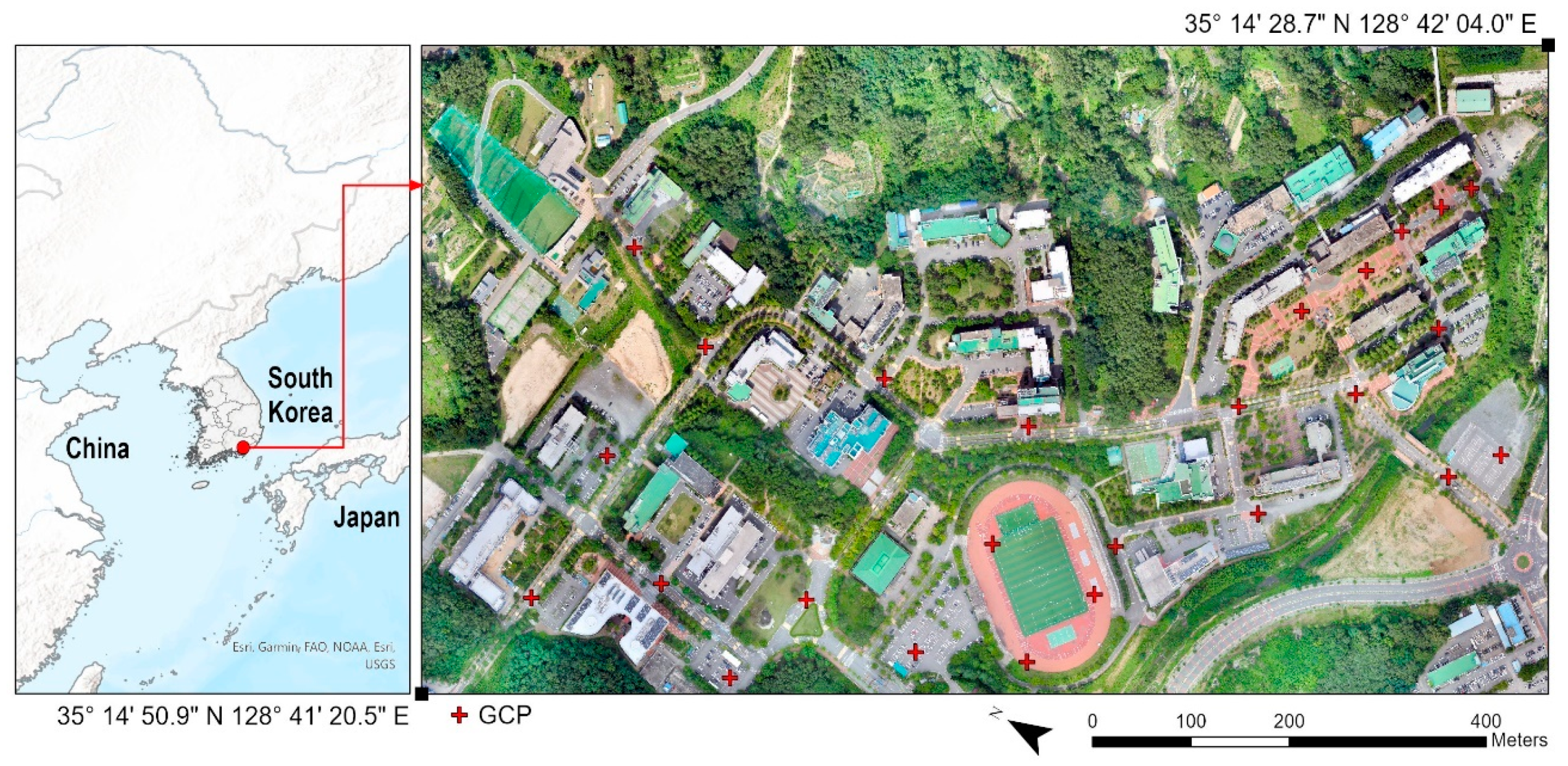
The entire campus of Changwon University in Changwon, Gyeongsangnam-do, South Korea, was selected as the target area. The university contains various land cover types within a relatively small area; thus, it was optimal to verify the applicability of urban land cover maps produced via UAV-derived imagery (Figure 1). The UAV imaging range was set as a rectangle of 623 m × 1138 m and included the area immediately outside the university. The local topography is surrounded by mountains, with an average elevation of ~600 m above sea level. Most university buildings are between five and eight stories, contain a wide pedestrian path made of sidewalk block material, as well as a road area with cars and pavement. In addition, there are numerous landscaping features, such as lawns, trees, etc.

Figure 1.
Study area (original UAV image-RGB).
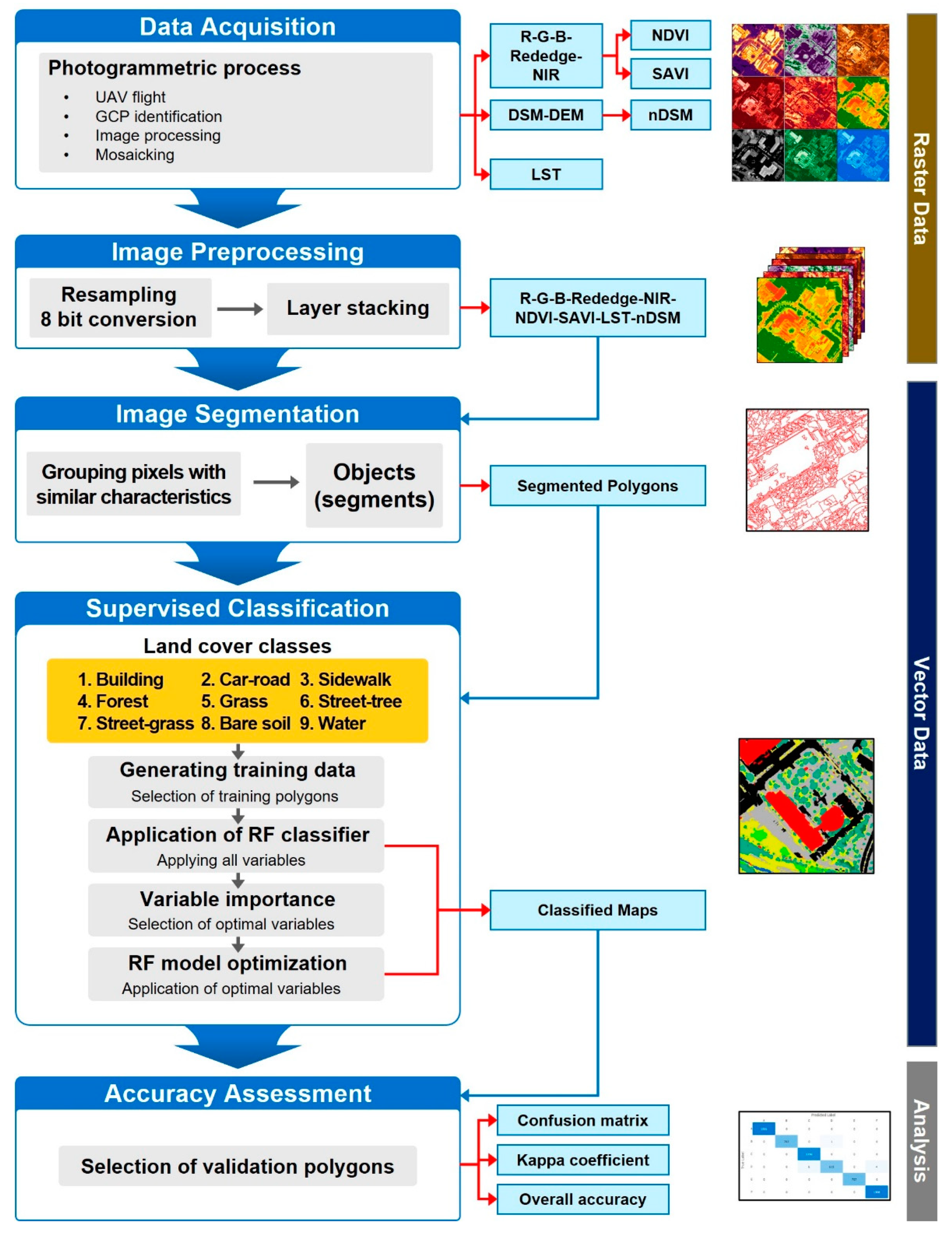
The research process here can be simplified into five main steps (Figure 2): data acquisition, image preprocessing, image segmentation, classification, and accuracy assessment. Essential data collection consisted of UAV flights to obtain GCPs for producing orthoimages so that multiple images could be overlapped for the same area. Image preprocessing was conducted to identify images and variables effective in classifying land cover types within this urban environment. To this end, the differences in the relative sizes of numerical data were eliminated so an identical weight could be assigned to all images (this is discussed in detail in Section 2.2). Next, objects were created by grouping pixels with similar characteristics through image segmentation and object creation. Accordingly, training data were produced, applied across all variables that could be extracted from the UAV imagery, and used to train an RF classifier to calculate variable importance. Through this process, the most effective images and variables for classifying land cover in urban areas were obtained, and the model was retrained according to this reduced image and variable number. Lastly, accuracy comparisons and verifications were carried out to assess the usefulness of classifying land cover in urban areas using UAV images and OBIA.

Figure 2.
Conceptual diagram of data acquisition, preprocessing, segmentation, classification, and validation steps implemented to derive an object-based land cover map for an urban environment from UAV imagery.
2.2. UAV Image Acquisition and Preprocessing
The UAV used in this study was a fixed-wing aircraft, eBeeX developed by Sensefly (Cheseaux-sur-Lausanne, Switzerland), with a weight of ~1.4 kg, and a 116 cm wingspan. The aircraft can fly at speeds of 40–110 km·h−1 for ≤90 min and can be equipped with various sensors such as RGB, thermal infrared, and 5-band multi-spectral sensors and built-in real-time/post-processed kinematic (RTK/PPK) functionality. We utilized Duet-T (RGB + Thermal) and RedEdge-MX (Red, Green, Blue, Rededge, NIR) imagers in this study. Filming was conducted on June 21, 2021, a notably clear sky day without clouds. The flights were conducted under the following conditions: for the installation of the RedEdge-MX sensor, the ground sample distance (GSD) was set to 13 cm·pixel−1; whereas that of the Duet-T sensor was set to 20 cm·pixel−1. Both vertical and horizontal redundancies were set to 75%. The 25 ground control points (GCPs) seen in Figure 1 were established for the aerial triangulation of the drone images.
The UAV photos collected were converted into orthoimages using Pix4D Mapper software v.4.4.12 developed by Pix4D (Prilly, Switzerland), preparing datasets of Red, Green, Blue, RedEdge, NIR band, digital surface model (DSM), digital elevation model (DEM), and land surface temperature (LST). The five band images acquired from the RedEdge-MX sensor were radiometrically corrected by a calibrated reflectance panel and downwelling light sensor; images of the panel taken before and after each flight were used to correct the reflectance values of the UAV images using known reflectance values in post-processing; the downwelling light sensor, which was mounted on top of the UAV to face upward, recorded the light conditions during flights and corrects the reflectance values of the UAV images along with the images of the panel in post-processing. Additionally, both the normalized difference vegetation index (NDVI) and soil adjusted vegetation index (SAVI) were derived according to Equations (1) and (2). NDVI is an indicator of vegetation obtained using red and NIR bands, where higher values indicate greater densities of live vegetation. Alternatively, SAVI is an index used to correct NDVI for the effect of soil brightness in areas with low vegetation cover. SAVI derived from Landsat satellite images employs a soil brightness correction factor (L) of 0.5 to accommodate most land cover types for adjusting the NIR and red band ratio [40]. Through a difference operation with DEM, which represents the surface height of the DSM excluding natural features, the normalized digital surface model (nDSM) was produced representing only the elevation of natural features, excluding the pure surface. Employing nDSM in the classification process assumes that a more effective classification of buildings and trees in the terrain is possible.
All produced images were resampled with a GSD of 15 cm·pixel−1 based on the multi-spectral images to identify street grass coverage planted between the roads for landscaping. Since various UAV images were produced, the units of pixel values of the images were different; For example, in the case of nDSM, the unit was meter, and in the case of LST, celsius (°C) was used. As Immitzer et al. [41] and Luca et al. [30] suggested, the relative size of numerical data was removed at this stage, and the data was normalized within a common range to reduce the influence of potential outliers at the segmentation and classification stage, and reflect all values to the same degree of importance. Therefore, all input layers were equally rescaled in a linear band with an 8-bit range from 0 to 255. Finally, since one raster image was required as input data for performing image segmentation, a layer stack process of merging RGB, RedEdge, NIR, NDVI, SAVI, LST, and nDSM was conducted.
2.3. Image Segmentation and Object Creation
Image segmentation is the process of grouping individual pixels in raster data with similar spectral and specific shape characteristics into a single object. The shape and size of an object can vary depending on the object-based weight setting [42]. This technique enabled the calculation of average pixel values by considering that adjacent pixel groups and the determination of pixels are included in each object. Image segmentation generalizes the area within the raster to retain all feature data as a larger, contiguous area rather than a finite unit of pixels [43]. Therefore, the reliability of OBIA is determined by appropriate image segmentation, and classification accuracy may vary depending on these results. Here, ArcGIS Pro v.2.8 developed by ESRI (Redlands, CA, USA) was used for image segmentation and the image with nine orthoimages stacked was used. During image segmentation, the weights used to create each object must be considered. Object creation can be adjusted by modifying spectral and spatial detail to values between 1 and 20. Spectral detail is the relative importance of separating objects on spectral characteristics; for example, a higher spectral detail value in a forested scene will result in greater discrimination between the different tree species. Spatial detail is the relative importance of separating objects based on spatial characteristics; a higher value is appropriate for a scene where features of interest are small and clustered together [44]. Image segmentation is designed to improve classification processing speed by reducing spectral complexities and large file sizes related to fine spatial resolution; however, since the direct relationship between the input weight value and image segmentation result is inherently multifaceted, the analyst must identify appropriate criteria and methods via trial and error [45,46]. If one detail among two weights is reduced, the corresponding raster data complexity and file size decrease. Generally, image segmentation with a great spectral detail and low spatial detail is preferred due to shorter processing times. In the case of smaller objects, it is possible to merge with the most similar adjacent segments by adjusting the minimum segment size to less than the object size. Here, the spectral detail was applied sequentially from 10 to 20 by units of 5, and the spatial detail was converted to units of 5 for object creation. Next, spectral and spatial details were adjusted by units of 1, the minimum segment size was sequentially applied from 20 to 60 by units of 10, and small object sizes were merged with adjacent objects to select final weights.
2.4. Land Cover Classification via Random Forest
Since land cover maps can provide primary research data at the urban level, the nine classes selected here were designed to capture urban environments (Figure 2): buildings, car-road, sidewalk, forest, grass, street-tree, street-grass, bare soil, and water; here, street-tree and street-grass refer to green space for landscaping purposes. Roads were subdivided into cars and pedestrians, including forests, street-trees, grass, and street-grass subdivisions. The reason is that air pollutants such as fine dust and NOx are emitted from the vehicle spaces but not from the sidewalks; thus, subclassifications were designed to specify pollutant-generating spaces. In addition, in the case of the street-tree and street-grass, if the area was below a certain threshold, it was classified as road cover, according to the land cover map of the Ministry of Environment of South Korea. Street-tree and street-grass were included, as these land cover types can be utilized for diverse aspects, such as lowering fine dust particulates, creating wind paths, and lowering the thermal environment of urban areas.
The statistical values assigned to objects from UAV-based images to classify land cover were as follows: count, area, mean, max, range, standard deviation (STD), sum, variety, majority, minority, median, percentile (PCT), and nearby mean STD (NMS). Through this process, 126 variables were derived by calculating 14 statistical values per image per object. This study attempted to differentiate street-trees from spectrally similar forests, as well as street-grass from grass, forest and grass maintained surrounding objects with similar spectral characteristics; whereas street-tree and street-grass exist together with non-vegetation roads, sidewalks, buildings, resulting in the substantial deviation of surrounding spectral properties. Accordingly, the NMS variable was added so that the mean value of the objects within 3 m could be compared via their standard deviation.
For the supervised classification training data, polygons in the range of 1000–5000 were constructed for the eight classes (excluding water). Only 165 polygons were selected for water, as the riverside vegetation covered most riverine areas. All trained polygons were manually selected through screen analysis while considering the distribution between land cover grades and shading for the various colors characterizing the study area.
RF is an automatic, machine learning algorithm proposed by Breiman [47] consisting of multiple decision tree sets and bootstrap aggregation (i.e., bagging). RF offers a method for combining basic classifiers trained on slightly different training data; for example, one decision tree is trained with identical samples, while another is trained without certain samples. Although individual decision trees can be highly sensitive to noise in the training data, the derived results, by voting multiple trees by lowering the correlation between the trees, show strong resistance to noise [48,49].
Although the RF classifier has numerous advantages, it is notably challenging to secure the precise explanatory power of independent on dependent variables as with most machine learning methods. Accordingly, increasing the variable number can make OBIA classification a highly subjective and time-intensive task [50,51]. To address this issue, measurements of varying importance were used to estimate which variables played the most crucial role in predictive performance, thereby optimizing variable selection.
Training data sample collection is essential for the RF classifier. Congalton and Green [52] emphasized the importance of collecting an adequate number of samples to maintain a statistically valid representation of map accuracy. Since the areal ratios of land cover are unequal, accuracy assessments can be statistically biased and imprecise despite sampling; proportionate numbers of samples per land cover item were collected in the present study. Among the 254,456 total image objects, 22,353 (8.8%) objects were selected as training data. For RF learning, the percentage of validation data among the training data was set to 30%. The number of trees in RF was set between the range of 100–1000, with a maximum depth of trees between 5 and 10, and the minimum leaf size was between 1 and 3. Through adjustments and alternations, an appropriate RF model was identified. Ultimately, the number of trees was set to 500, with a maximum depth of 10, and a minimum leaf size of 2. Variable importance was then calculated, the variables were optimized, retrained, and compared to the original RF model under the same conditions.
The random points used for accuracy verification of the classified land cover maps are shown in Figure 3. By creating a confusion matrix of classification accuracy, the producer’s, user’s, and overall accuracy were calculated. For accuracy verification, 500 visually interpreted verification points were randomly selected based on the original UAV images.
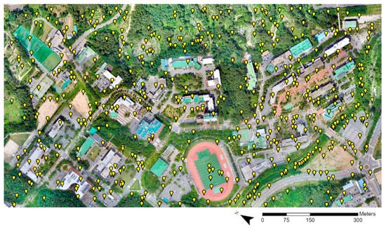
Figure 3.
Random point locations for accuracy verification.
3. Results and Discussion
3.1. Results of UAV Flight
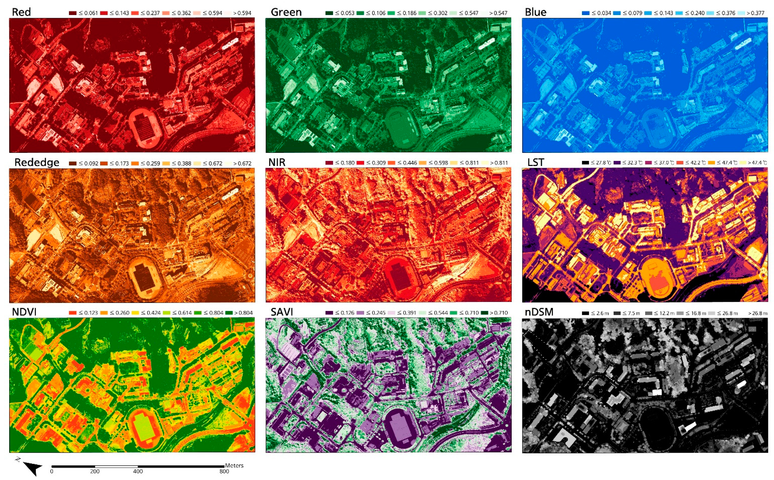
As a result of UAV image collection, RGB, RedEdge, and NIR images were collected from the Rededge-MX sensor totaling 5925 images. An additional 1132 RGB and LST images were collected from the Duet-T sensor. Figure 4 presents the image results produced by mosaicking the collected images; nine images were produced and assessed. As a result of the geometric correction of the images using the GCPs, the Duet-T sensor-based images showed a root-mean-square error (RMSE) of 0.033 m and 0.048 m in the x- and y-directions, respectively. Alternatively, the Rededge-MX sensor-based images maintained an RMSE of 0.056 m and 0.054 m in the x- and y-directions, respectively.
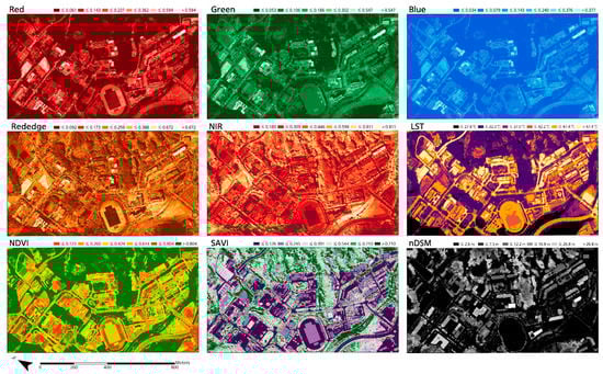
Figure 4.
UAV image production results.
3.2. Optimal Image Segmentation Weight
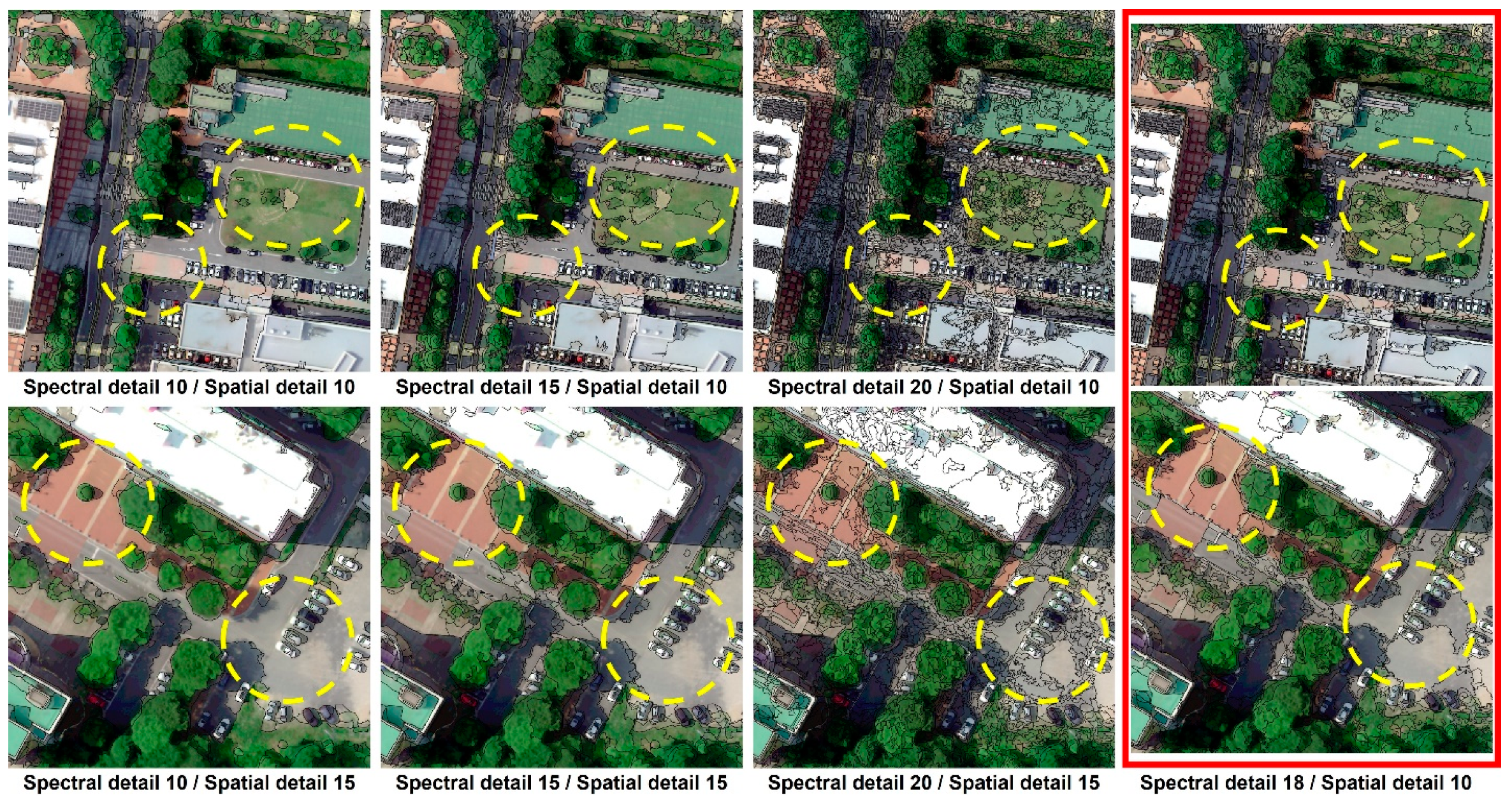
When selecting image segmentation weights, at spectral detail 10, the boundaries between road and grass were obscured (Figure 5); while at spectral detail 15, there were certain sections where road and sidewalk were not readily distinguished. At spectral detail 20, there was a tendency for objects to be (too) finely demarcated, even within the same land cover class. In such cases, the boundaries between land cover classes are apparent; however, since the object size is tiny, it may become susceptible to image noise. From spectral or spatial detail 15, car-road and sidewalk began to be distinguished, although there was no boundary between the asphalt-paved car-road and bare soil (consisting of gravel). Accordingly, the conditions at which the boundary between car-road and bare soil became clear were explored by increasing spectral detail. A more detailed adjustment revealed that these boundaries were clear for each land cover class under a spectral detail of 18 and spatial detail of 10, without objects being formed in excessive detail. When the minimum segment size was set to 40, it was assumed that the object size was subdivided into an appropriate size; indeed, as the boundary of the street-grass became clear, this weight was selected.
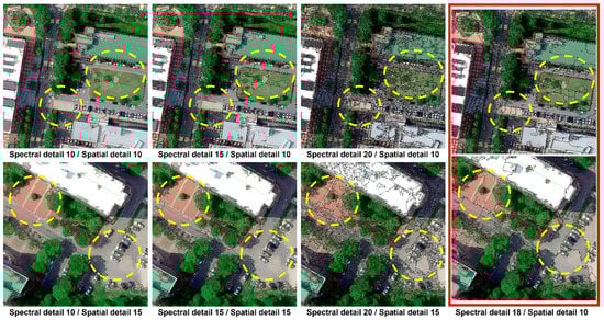
Figure 5.
Image segmentation results.
3.3. Land Cover Map Classification Results
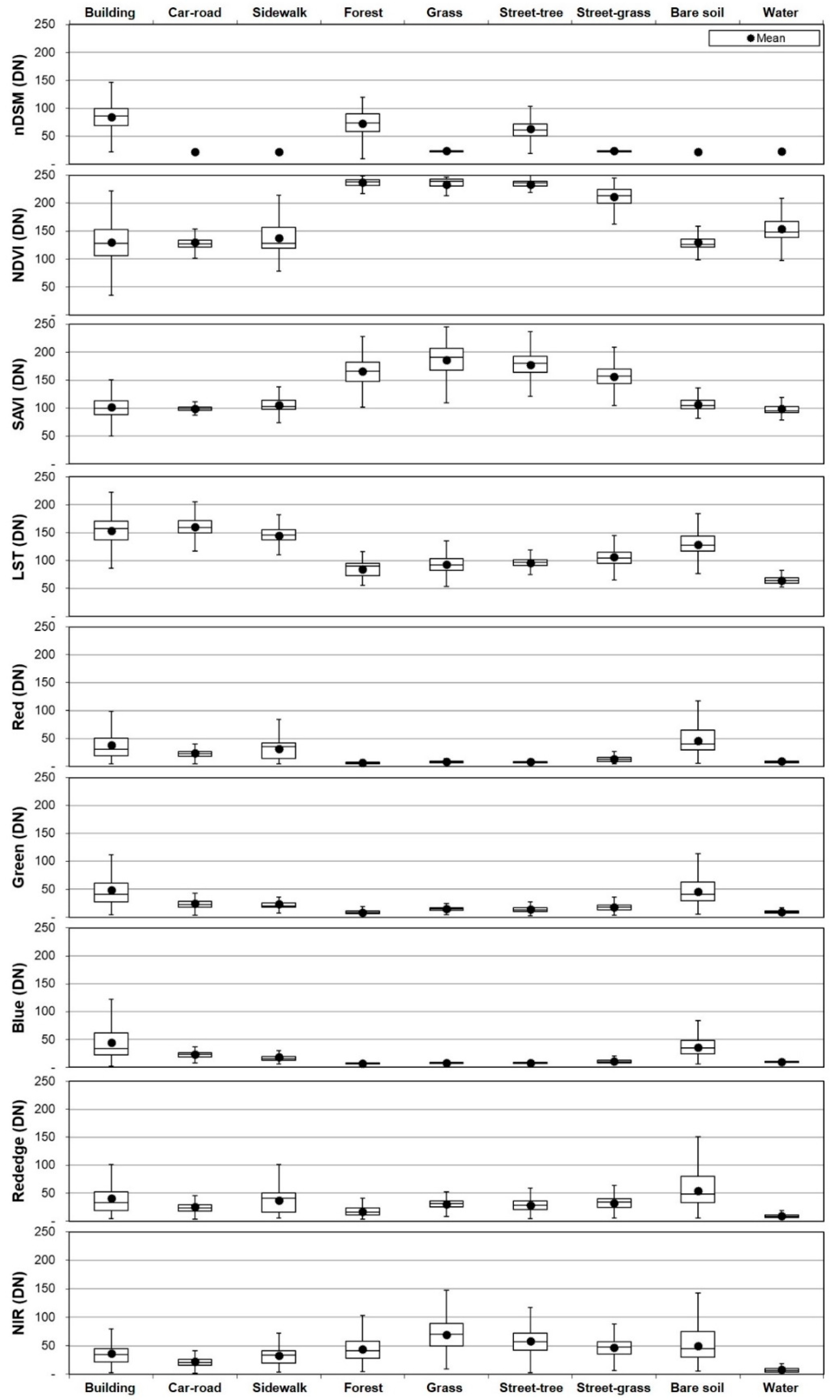
Figure 6 shows the characteristics of the training data per class. For nDSM, the interquartile ranges of building, forest, and street-tree were 69 to 100, 58 to 90, and 51 to 72, respectively, and other land cover types had almost no ranges.; due to the characteristics of the natural features, building, forest, and street-tree were clearly distinguished from other land cover types. NDVI and SAVI showed distinctly higher trends in the vegetation classes. For NDVI, the interquartile range of the vegetation classes was 231 to 243, and the highest third quartile of other land cover types was under 167. In the case of SAVI, the interquartile range of the vegetation classes was 144 to 207, and the highest third quartile of other land cover types was under 114. Notably, the NDVI of the street-grass presented a greater range of values due to the varying proportion of exposed grass and soil components. Furthermore, most ranges nearly overlapped for the non-vegetation classes, and it was found that although vegetation and non-vegetation could be broadly distinguished using NDVI and SAVI, deciphering further detail was challenging, such as car-road, sidewalk, and bare soil. For LST, the interquartile range of land cover types were 137 to 171 (building), 150 to 172 (car-road), 137 to 155 (sidewalk), 73 to 95 (forest), 83 to 104 (grass), 91 to 102 (street-tree), 95 to 115 (street-grass), 117 to 144 (bare soil), and 60 to 69 (water), respectively. Water was clearly distinguished and classified by significantly lower values, followed by vegetation (e.g., forest and grass) still within a low range. Artificial land cover types, such as building and car-road maintained higher LSTs; whereas the range of bare soil values was widely distributed from vegetation to artificial cover types. For the Red, Green and Blue images, the boxplots of car-road, sidewalk, and bare soil continuously overlapped for all images, save for blue band reflectance values. In the case of Blue image, the interquartile range of car-road, sidewalk, and bare soil were 19 to 26, 13 to 20, and 24 to 48, resplectively; although the boxplots overlapped a little, they were more differentiated than the Red and Green images. For the NIR and rededge wavelengths, the range of boxplots for most classes overlapped (except for water). Notably, the car-road class, mainly consisting of black asphalt, had a narrower boxplot range than the sidewalk composed of various colored blocks.
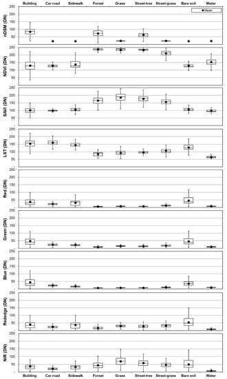
Figure 6.
Training data characteristics based on land cover.
As a result of training the RF model using all 126 variables, the top 40 most important variables (importance > 0.6%; Figure 7) were ranked as follows: nDSM (there are 8 variables in the top 40), NDVI (7), LST (7), SAVI (6), Blue (6), Green (4), Red (1), and Rededge (1). nDSM and NDVI occupied the first to twelfth most important variables, whereas those from 13th onwards were diverse images and statistical values. Presumably, nDSM distinguished building from trees via height measurements, while NDVI was effective in distinguishing vegetation from non-vegetation classes. Among the vegetation indices, NDVI showed higher importance than SAVI, likely as a result of NDVI presenting fewer overlapping sections between the ranges of forest, grass, and street-tree. LST was distributed between the ranks of 16–33, and as shown in the training data characteristics, it was an important factor for distinguishing car-road, and sidewalk, as well as water. Most previous studies have used multi-spectral images and vegetation indices such as NDVI [33,34,35] for larger, regional-scale analyses; however, the results here suggest that LST can also be used in urban area classification. As for previous studied that compared LST data acquired using UAVs with in-situ LSTs, Song and Park (2020) [10] measured and compared UAV LST and in-situ LST; the UAV LSTs exhibited differences of 4.5 °C (July) and 5.4 °C (August) between sidewalk and car-road; for effective LST image utilization, it is considered best that LST image is taken at noon in summer, when the influence of shadow is minimal due to the highest solar altitude. Among the single spectral wavelengths, the blue image occupied the highest importance rank, likely due to its increased ability to distinguish car-road, sidewalk, and bare soil. The statistical values of variable importance were as follows: PCT75 (6 variables), mean (6), NMS (5), majority (5), median (5), max (5), min (4), minority (3), and STD (1). In nDSM, median, PCT75, and mean occupied the high ranks, while in NDVI, mean, PCT75, and median were the most important. In NMS used to distinguish street-tree from street-grass, nDSM and green images were the most important.
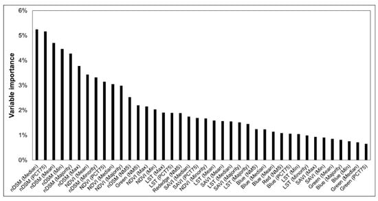
Figure 7.
Most important 40 variables out of the 126 assessed.
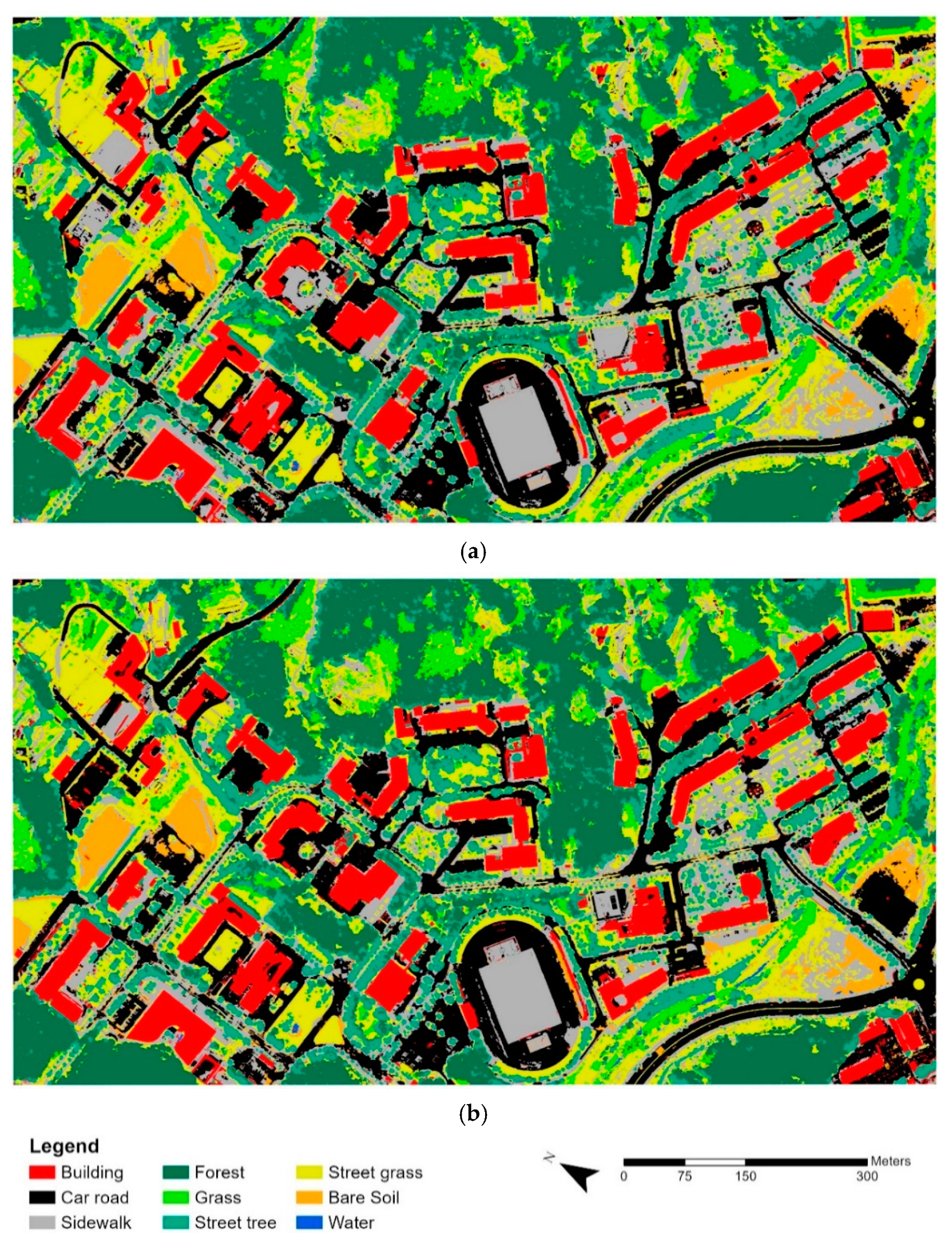
Through variable importance, the model was reduced and optimized to the six images of nDSM, NDVI, SAVI, LST, blue, and green, and seven variables of PCT75, mean, NSM, median, majority, max, and min. The results of applying these models to the entire target areas can be found in Figure 8. When predicting land cover through the model using all 126 variables, the area ratio per land cover class was: forest (19.2%) > car-road (16.8%) > street-grass (16.6%) > street-tree (14.8%) > sidewalk (13.5%) > building (11.5%) > grass (5.3%) > bare soil (2.2%) > and water (0.1%); whereas in the optimized RF of reduced variables, the results were: forest (19.1%) > car-road (17.6%) > street-grass (16.4%) > street-tree (14.7%) > sidewalk (12.2%) > building (11.6%) > grass (5.8%) > bare soil (2.5%) > and water (0.1%), indicating that the overall area ratios were similar (≤1%), except for sidewalk; further, there was no significant change in classification results despite the reduced number of variables.
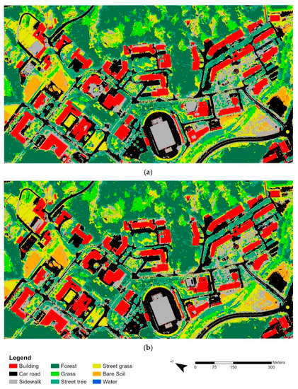
Figure 8.
Results of applying the RF model to the entire target sites: (a) Initial RF with 126 variables (b) Optimized RF with reduced variable number.
As a result of quantitatively analyzing land cover classification, forest and street-trees were well distinguished. In contrast, water occupied a tiny percentage of the target area, indicative of classification accuracy despite the least training data. It was found that among the artificial cover types, building and car-roads were well-classified, and it was confirmed that car-road and sidewalk were accurately separated; however, there was a tendency to classify car-road as a sidewalk in some areas. As shadows are one of the most common problems hindering accurate data extraction in remote sensing analyses, additional studies on shadow detection and correction are required [53,54]. Indeed, a small path in the forest was classified as a sidewalk, and there was a tendency to misclassify the surrounding grass as street-grass. Furthermore, there was a tendency to classify bare soil as a sidewalk.
3.4. Accuracy Verification
As a result of the accuracy verification, the Kappa coefficient of the initial RF containing all variables was 0.728 (76.0% overall accuracy). Comparatively, the Kappa coefficient of the optimized RF was 0.721 (75.4% overall accuracy), indicating that the accuracy did not decrease significantly despite the reduced variable number (Table 1 and Table 2). The user’s accuracy based on variable optimization was within ±3% for building, car-road, sidewalk, forest, grass, street-tree, and street-grass, indicating no significant difference compared to the initial RF. This accuracy increased to 4.9% for water. There was also an increased tendency for the sidewalk to be classified as bare soil when compared to the initial RF, wherein accuracy decreased by 13.8%. The producer’s accuracy was also within ±3% for building, forest, street-tree, bare soil, and water, similarly suggesting there was no significant change compared to the initial RF. Furthermore, the producer’s accuracy for sidewalk and street-grass decreased by −7.5 and −6.0%, respectively; whereas the accuracy for grass and car-road increased by 7.0% and 5.6%, respectively. Therefore, in terms of accuracy changes, there was not a large impact of the reduced variable number on buildings, forests, and street-trees, corroborating the use of nDSM and NDVI in previous studies to accurately classify buildings and forests [55,56,57]. Vanhuysse et al. [58] reported that when nDSM was used as input data, there were improvements in the quantitative and qualitative analysis of building and other classification results. Therefore, in the present study, buildings, forests, and street-trees showed little change despite variable optimization, as nDSM and NDVI, which occupied high ranks of variable importance, were included.

Table 1.
Confusion matrix for the initial RF.
Table 2.
Confusion matrix for the optimized RF.
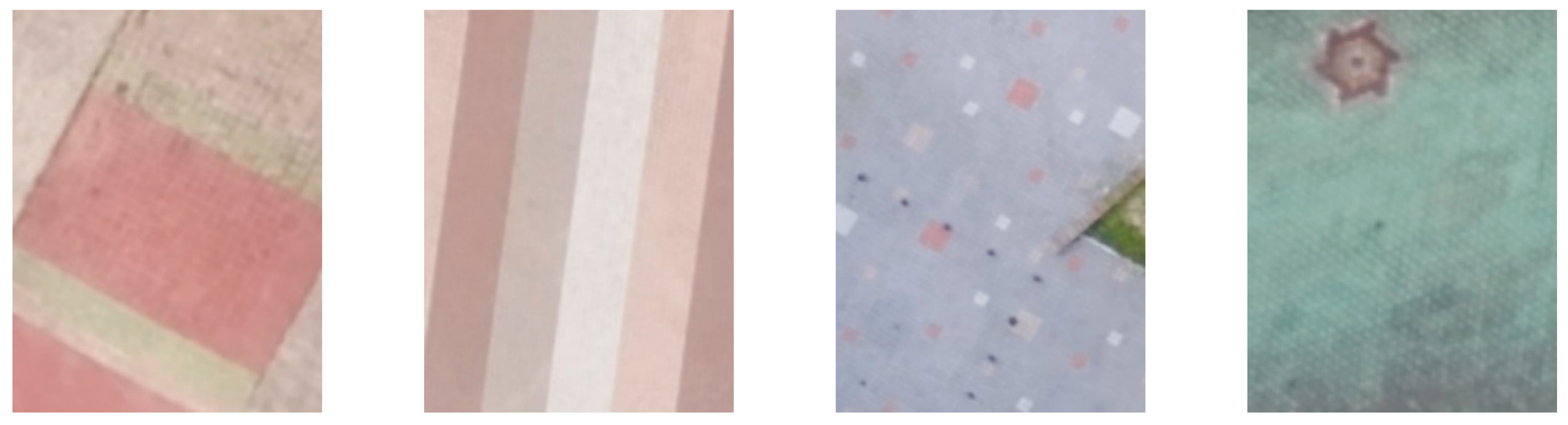
In the optimized RF, building and water classes maintained >90% of the user and producer’s accuracy. As mentioned above, buildings were mainly identified through nDSM, while water showed the most significant difference from other land cover types with different LSTs among the optimized variables (Figure 6). The classification accuracy of vegetation was likely high due to NDVI, as indicated by the overlapping boxplots for these areas. When car-road and sidewalk were classified as a road, the producer and user accuracies were 89.6% and 80.0%, respectively, similar to the classification accuracy results of other studies (75–95%) [57,59,60,61]. However, as sidewalks were over-predicted in the present study, the user’s accuracy was low (65.7%). There was a tendency to misclassify bare soil with similar spectral characteristics as a sidewalk since the blocks constituting the sidewalk within the target site encompassed various colors, such as beige, red, green, and gray (Figure 9). Accordingly, 46% of the reference data of bare soil was classified as a sidewalk, and the producer’s accuracy of the bare soil was very low (31.5%). When forest and street trees were classified are merged into a single item and classified as tree, the user’s and producer’s accuracies increased to 97.2% and 96.3%, respectively. In contrast, if a tree was subdivided into forest and street-trees, the accuracy decreased due to misclassification between these two items. When assessing these areas via visual interpretation, they were judged to be affected by tree shadow. Notably, it is assumed that acknowledgment of this error can be improved by including forest-type maps as auxiliary data in the future.
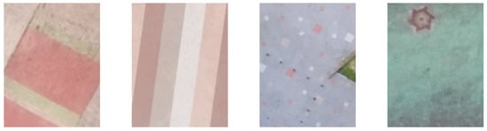
Figure 9.
Example of sidewalk block types in the target site.
4. Conclusions
Land cover maps contain critical spatial data necessary for urban environmental evaluation and research; however, their utilization has been limited for small- and medium-sized areas due to limited temporal data resolution, accuracy, and high production costs. In this study, as a measure for addressing such limitations, effective images for constructing land cover maps were analyzed via UAV, and the applicability of the land cover classification method was confirmed. The primary research achievements were as follows:.Nine UAV-derived images were used for OBIA: red, green, blue, RedEdge, NIR, LST, NDVI, SAVI, and nDSM. The optimal image segmentation weights were selected as spectral detail 18, spatial detail 10, and a minimum segment size of 40. While using 126 variables for training the initial RF and computing variable importance up to the 40th, the most influential variables were nDSM > NDVI > LST > SAVI > blue > green > red > rededge. nDSM was assumed to be effective for distinguishing between buildings and trees, whereas NDVI distinguished vegetation and non-vegetation classes and maintained significantly greater priority than SAVI, which ideally minimized the effects of soil brightness (a notably variable characteristic). Variable importance LST was distributed between the 16th and 33rd places. Indeed, although most multi-spectral images and vegetation indices have been mainly used for land cover classification, it was shown that LST images could be effectively used for land cover classification of urban areas. It was an important factor for distinguishing car-road, and sidewalk, as well as water. For effective LST image utilization, it is considered best that LST image is taken at noon in summer, when the influence of shadow was minimal due to the highest solar altitude. Among the images containing a single spectral wavelength, the blue image maintained the highest level of variable importance to distinguish car-road, sidewalk, and bare soil. Finally, in terms of NMS, which was used to distinguish street-tree and street-grass, the priority of nDSM and green images ranked high.
Comparing the land cover classification results of the initial RF using all 126 variables with the optimized RF obtained via variable reduction, the difference in the overall area ratio was 1.3%. Indeed, despite the reduced variable number, there was no significant change in the overall classification results. As a result of the accuracy verification, the Kappa coefficient of the initial RF was 0.728; whereas that of the optimized RF was 0.721. When examining the accuracy changes for each land cover item, it was found that buildings, forests, and street-trees were not significantly affected, presumably due to the influence of nDSM and NDVI, which maintained higher variable importance. When car-road and sidewalk were classified as a road (as often observed in other studies), producer and user accuracy were 89.6% and 80.0%, respectively (similar to other studies). There was, however, a tendency to misclassify bare soil as a sidewalk since the sidewalk blocks were made of various colors. When forest and street trees were classified are merged into a single item and classified as tree, the user and producer accuracies were 97.2% and 96.3%, respectively. However, the accuracy decreased when subdividing these classes into forest and street-trees. Visual interpretation revealed that shadows had a significant effect on the trees present. Thus, it was judged that this error can be improved by incorporating a map of forest type as ancillary data.
The acquisition of image data using UAV maintains fewer spatiotemporal constraints than satellite and other aerial imagery forms. It also becomes possible to obtain more accurate data than the time and costs required for data processing. It was further judged that applying the object-based land cover classification technique using UAV imagery can contribute to urban environmental research. However, since this study created a land cover map solely with images from a single period, it is necessary to verify the feasibility of constructing a time series of land cover maps through further research, in addition to exploring additional methods for improving classification accuracy. Generally, forests should have a minimum area and tree coverage fraction, but this study was not taken into account here. Further research will be needed to improve this.
Author Contributions
Conceptualization, G.P., B.S., K.P. and H.L.; methodology, G.P., B.S. and K.P.; formal analysis, G.P.; investigation, G.P. writing—original draft preparation, G.P. and B.S.; writing—review and editing, G.P., B.S., K.P. and H.L.; supervision, H.L. All authors have read and agreed to the published version of the manuscript.
Funding
This results was supported by “Regional Innovation Strategy (RIS)” through the National Research Foundation of Korea(NRF) funded by the Ministry of Education(MOE)(2021RIS-003) and the National Research Foundation of Korea(NRF) grant funded by the Korea government(MSIT) (No. NRF-2019R1F1A1063921).
Institutional Review Board Statement
Not applicable.
Informed Consent Statement
Not applicable.
Data Availability Statement
Not applicable.
Conflicts of Interest
The authors declare no conflict of interest.
References
- Song, B.; Park, K. Temperature trend analysis associated with land-cover changes using time-series data (1980–2019) from 38 weather stations in South Korea. Sustain. Cities Soc. 2021, 65, 102615. [Google Scholar] [CrossRef]
- De Castro, A.I.; Torres-Sánchez, J.; Peña, J.M.; Jiménez-Brenes, F.M.; Csillik, O.; López-Granados, F. An automatic random forest-OBIA algorithm for early weed mapping between and within crop rows using UAV imagery. Remote Sens. 2018, 10, 285. [Google Scholar] [CrossRef] [Green Version]
- Kim, E.J.; Won, J.; Kim, J. Is Seoul walkable? Assessing a walkability score and examining its relationship with pedestrian satisfaction in Seoul, Korea. Sustainability 2019, 11, 6915. [Google Scholar] [CrossRef] [Green Version]
- Takahashi Miyoshi, G.; Imai, N.N.; Garcia Tommaselli, A.M.; Antunes de Moraes, M.V.; Honkavaara, E. Evaluation of hyperspectral multitemporal information to improve tree species identification in the highly diverse Atlantic Forest. Remote Sens. 2020, 12, 244. [Google Scholar] [CrossRef] [Green Version]
- Song, B.; Park, K. Analysis of spatiotemporal urban temperature characteristics by urban spatial patterns in Changwon City, South Korea. Sustainability 2019, 11, 3777. [Google Scholar] [CrossRef] [Green Version]
- Yoo, S.H.; Lee, J.S.; Bae, J.S.; Sohn, H.G. Automatic generation of land cover map using residual U-Net. KSCE J. Civil Environ. Eng. Res. 2020, 40, 535–546. [Google Scholar] [CrossRef]
- Kim, J.; Song, Y.; Lee, W.K. Accuracy analysis of multi-series phenological landcover classification using U-net-based deep learning model—Focusing on the Seoul, Republic of Korea. Korean J. Remote Sens. 2021, 37, 409–418. [Google Scholar] [CrossRef]
- Scaioni, M.; Longoni, L.; Melillo, V.; Papini, M. Remote sensing for landslide investigations: An overview of recent achievements and perspectives. Remote Sens. 2014, 6, 9600–9652. [Google Scholar] [CrossRef] [Green Version]
- Van Iersel, W.; Straatsma, M.; Addink, E.; Middelkoop, H. Monitoring height and greenness of non-woody floodplain vegetation with UAV time series. ISPRS J. Photogramm. Remote Sens. 2018, 141, 112–123. [Google Scholar] [CrossRef]
- Song, B.; Park, K. Verification of accuracy of unmanned aerial vehicle (UAV) land surface temperature images using in-situ data. Remote Sens. 2020, 12, 288. [Google Scholar] [CrossRef] [Green Version]
- Park, G.; Park, K.; Song, B. Spatio-temporal change monitoring of outside manure piles using unmanned aerial vehicle images. Drones 2021, 5, 1. [Google Scholar] [CrossRef]
- Song, B.; Park, K. Detection of aquatic plants using multispectral UAV imagery and vegetation index. Remote Sens. 2020, 12, 387. [Google Scholar] [CrossRef] [Green Version]
- Uysal, M.; Toprak, A.S.; Polat, N. DEM generation with UAV photogrammetry and accuracy analysis in Sahitler Hill. Measurement 2015, 73, 539–543. [Google Scholar] [CrossRef]
- Ferrer-González, E.; Agüera-Vega, F.; Carvajal-Ramírez, F.; Martínez-Carricondo, P. UAV photogrammetry accuracy assessment for corridor mapping based on the number and distribution of ground control points. Remote Sens. 2020, 12, 2447. [Google Scholar] [CrossRef]
- Prado Osco, L.; Marques Ramos, A.P.; Roberto Pereira, D.; Akemi Saito Moriya, É.; Nobuhiro Imai, N.; Takashi Matsubara, E.; Estrabis, N.; de Souza, M.; Marcato Junior, J.; Gonçalves, W.N.; et al. Predicting Canopy nitrogen content in citrus-trees using random forest algorithm associated to spectral vegetation indices from UAV-imagery. Remote Sens. 2019, 11, 2925. [Google Scholar] [CrossRef] [Green Version]
- Siebert, S.; Teizer, J. Mobile 3D mapping for surveying earthwork projects using an unmanned aerial vehicle (UAV) system. Autom. Constr. 2014, 41, 1–14. [Google Scholar] [CrossRef]
- Su, T.C. A study of a matching pixel by pixel (MPP) algorithm to establish an empirical model of water quality mapping, as based on unmanned aerial vehicle (UAV) images. Int. J. Appl. Earth Obs. Geoinf. 2017, 58, 213–224. [Google Scholar] [CrossRef]
- Nex, F.; Remondino, F. UAV for 3D mapping applications: A review. Appl. Geomat. 2014, 6, 1–15. [Google Scholar] [CrossRef]
- Al-Najjar, H.A.H.; Kalantar, B.; Pradhan, B.; Saeidi, V.; Halin, A.A.; Ueda, N.; Mansor, S. Land cover classification from fused DSM and UAV images using convolutional neural networks. Remote Sens. 2019, 11, 1461. [Google Scholar] [CrossRef] [Green Version]
- Yao, H.; Qin, R.; Chen, X. Unmanned aerial vehicle for remote sensing applications—A review. Remote Sens. 2019, 11, 1443. [Google Scholar] [CrossRef] [Green Version]
- Torresan, C.; Berton, A.; Carotenuto, F.; Di Gennaro, S.F.; Gioli, B.; Matese, A.; Miglietta, F.; Vagnoli, C.; Zaldei, A.; Wallace, L. Forestry applications of UAVs in Europe: A review. Int. J. Remote Sens. 2017, 38, 2427–2447. [Google Scholar] [CrossRef]
- Crommelinck, S.; Bennett, R.; Gerke, M.; Nex, F.; Yang, M.Y.; Vosselman, G. Review of automatic feature extraction from high-resolution optical sensor data for UAV-based cadastral mapping. Remote Sens. 2016, 8, 689. [Google Scholar] [CrossRef] [Green Version]
- Timm, B.C.; McGarigal, K. Fine-scale remotely-sensed cover mapping of coastal dune and salt marsh ecosystems at Cape Cod National Seashore using random forests. Remote Sens. Environ. 2012, 127, 106–117. [Google Scholar] [CrossRef]
- Hayes, M.M.; Miller, S.N.; Murphy, M.A. High-resolution landcover classification using random forest. Remote Sens. Lett. 2014, 5, 112–121. [Google Scholar] [CrossRef]
- Tamouridou, A.; Alexandridis, T.; Pantazi, X.; Lagopodi, A.; Kashefi, J.; Moshou, D. Evaluation of UAV imagery for mapping Silybum marianum weed patches. Int. J. Remote Sens. 2017, 38, 2246–2259. [Google Scholar] [CrossRef]
- Blaschke, T. Object based image analysis for remote sensing. ISPRS J. Photogramm. Remote Sens. 2010, 65, 2–16. [Google Scholar] [CrossRef] [Green Version]
- Kim, H.O.; Yeom, J.M. Effect of red-edge and texture features for object-based paddy rice crop classification using RapidEye multi-spectral satellite image data. Int. J. Remote Sens. 2014, 35, 7046–7068. [Google Scholar] [CrossRef]
- Torres-Sánchez, J.; López-Granados, F.; Peña, J.M. An automatic object-based method for optimal thresholding in UAV images: Application for vegetation detection in herbaceous crops. Comput. Electron. Agric. 2015, 114, 43–52. [Google Scholar] [CrossRef]
- Blaschke, T.; Hay, G.J.; Kelly, M.; Lang, S.; Hofmann, P.; Addink, E.; Queiroz Feitosa, R.; van der Meer, F.; van der Wer, H.; van Coillie, F.; et al. Geographic object-based image analysis–towards a new paradigm. ISPRS J. Photogramm. Remote Sens. 2014, 87, 180–191. [Google Scholar] [CrossRef] [Green Version]
- Luca, G.D.; Silva, J.M.N.; Cerasoli, S.; Araújo, J.; Campos, J.; Fazio, S.; Modica, G. Object-based land cover classification of cork oak woodlands using UAV imagery and Orfeo ToolBox. Remote Sens. 2019, 11, 1238. [Google Scholar] [CrossRef] [Green Version]
- Ma, L.; Li, M.; Ma, X.; Cheng, L.; Du, P.; Liu, Y. A review of supervised object-based land-cover image classification. ISPRS J. Photogramm. Remote Sens. 2017, 130, 277–293. [Google Scholar] [CrossRef]
- Ahmed, O.S.; Shemrock, A.; Chabot, D.; Dillon, C.; Williams, G.; Wasson, R.; Franklin, S.E. Hierarchical land cover and vegetation classification using multispectral data acquired from an unmanned aerial vehicle. Int. J. Remote Sens. 2017, 38, 2037–2052. [Google Scholar] [CrossRef]
- Kilwenge, R.; Adewopo, J.; Sun, Z.; Schut, M. UAV-based mapping of banana land area for village-level decision-support in Rwanda. Remote Sens. 2021, 13, 4985. [Google Scholar] [CrossRef]
- Natesan, S.; Armenakis, C.; Benari, G.; Lee, R. Use of UAV-borne spectrometer for land cover classification. Drones 2018, 2, 16. [Google Scholar] [CrossRef] [Green Version]
- Lv, Z.; Shi, W.; Benediktsson, J.A.; Ning, X. Novel Object-based filter for improving land-cover classification of aerial imagery with very high spatial resolution. Remote Sens. 2016, 8, 1023. [Google Scholar] [CrossRef] [Green Version]
- Geipel, J.; Link, J.; Claupein, W. Combined spectral and spatial modeling of corn yield based on aerial images and crop surface models acquired with an unmanned aircraft system. Remote Sens. 2014, 6, 10335–10355. [Google Scholar] [CrossRef] [Green Version]
- Lu, D.S.; Mausel, P.; Batistella, M.; Moran, E. Comparison of land-cover classification methods in the Brazilian Amazon Basin. Photogramm. Eng. Remote Sens. 2004, 70, 723–731. [Google Scholar] [CrossRef] [Green Version]
- Zhang, H.; Li, J.; Wang, T.; Lin, H.; Zheng, Z.; Li, Y.; Lu, Y. A manifold learning approach to urban land cover classification with optical and radar data. Landsc. Urban Plan. 2018, 172, 11–24. [Google Scholar] [CrossRef]
- Lu, D.; Weng, Q. Use of impervious surface in urban land-use classification. Remote Sens. Environ. 2006, 102, 146–160. [Google Scholar] [CrossRef]
- USGS. Available online: https://www.usgs.gov/landsat-missions/landsat-soil-adjusted-vegetation-index (accessed on 22 December 2021).
- Immitzer, M.; Vuolo, F.; Atzberger, C. First experience with Sentinel-2 data for crop and tree species classifications in central Europe. Remote Sens. 2016, 8, 166. [Google Scholar] [CrossRef]
- Kindu, M.; Schneider, T.; Teketay, D.; Knoke, T. Land use/land cover change analysis using object-based classification approach in Munessa-Shashemene landscape of the Ethiopian Highlands. Remote Sens. 2013, 5, 2411–2435. [Google Scholar] [CrossRef] [Green Version]
- Dronova, I.; Gong, P.; Wang, L. Object-based analysis and change detection of major wetland cover types and their classification uncertainty during the low water period at Poyang Lake, China. Remote Sens. Environ. 2011, 115, 3220–3236. [Google Scholar] [CrossRef]
- ESRI. Segmentation in ArcGIS Pro. Available online: https://pro.arcgis.com/en/pro-app/latest/help/analysis/image-analyst/segmentation.htm (accessed on 23 February 2022).
- Zhou, W.; Troy, A. An object-oriented approach for analysing and characterizing urban landscape at the parcel level. Int. J. Remote Sens. 2008, 29, 3119–3135. [Google Scholar] [CrossRef]
- Qian, Y.; Zhou, W.; Yan, J.; Li, W.; Han, L. Comparing machine learning classifiers for object-based land cover classification using very high resolution imagery. Remote Sens. 2015, 7, 153–168. [Google Scholar] [CrossRef]
- Breiman, L. Random forests. Mach. Learn. 2001, 45, 5–32. [Google Scholar] [CrossRef] [Green Version]
- Cutler, D.R.; Edwards, T.C.; Beard, K.H.; Cutler, A.; Hess, K.T.; Gibson, J.; Lawler, J.J. Random forests for classification in ecology. Ecology 2007, 88, 2783–2792. [Google Scholar] [CrossRef]
- Haas, J.; Ban, Y. Urban growth and environmental impacts in Jing-Jin-Ji, the Yangtze, River Delta and the Pearl River Delta. Int. J. Appl. Earth Obs. Geoinf. 2014, 30, 42–55. [Google Scholar] [CrossRef]
- Belgiu, M.; Drăguţ, L. Random forest in remote sensing: A review of applications and future directions. ISPRS J. Photogramm. Remote Sens. 2016, 114, 24–31. [Google Scholar] [CrossRef]
- Belgiu, M.; Drăguţ, L. Comparing supervised and unsupervised multiresolution segmentation approaches for extracting buildings from very high resolution imagery. ISPRS J. Photogramm. Remote Sens. 2014, 96, 67–75. [Google Scholar] [CrossRef] [Green Version]
- Congalton, R.G.; Green, K. Assessing the Accuracy of Remotely Sensed Data: Principles and Practices; Third CRC Press Taylor & Francis Group: Boca Raton, FL, USA, 2019; Volume 48. [Google Scholar]
- Shahtahmassebi, A.; Yang, N.; Wang, K.; Moore, N.; Shen, Z. Review of shadow detection and de-shadowing methods in remote sensing. Chin. Geograph. Sci. 2013, 23, 403–420. [Google Scholar] [CrossRef] [Green Version]
- Milas, A.S.; Arend, K.; Mayer, C.; Simonson, M.A.; Machey, S. Different colours of shadows: Classification of UAV images. Int. J. Remote Sens. 2017, 38, 3084–3100. [Google Scholar] [CrossRef]
- Gage, E.A.; Cooper, D.J. Urban forest structure and land cover composition effects on land surface temperature in a semi-arid suburban area. Urban For. Urban Green. 2017, 28, 28–35. [Google Scholar] [CrossRef]
- Hiscock, O.H.; Back, Y.; Kleidorfer, M.; Urich, C. A GIS-based land cover classification approach suitable for fine-scale urban water management. Water Resour. Manag. 2021, 35, 1339–1352. [Google Scholar] [CrossRef]
- Hai-yang, Y.U.; Gang, C.; Xiao-san, G.E.; Xiao-ping, L.U. Object oriented land cover classification using ALS and GeoEye imagery over mining area. Trans. Nonferr. Metal. Soc. Chin. 2011, 21 (Suppl. S3), s733–s737. [Google Scholar] [CrossRef]
- Vanhuysse, S.; Grippa, T.; Lennert, M.; Wolff, E.; Idrissa, M. Contribution of nDSM derived from VHR stereo imagery to urban land-cover mapping in Sub-Saharan Africa. In Proceedings of the 2017 Joint Urban Remote Sensing Event (JURSE), Dubai, United Arab Emirates, 6–8 March 2017; pp. 1–4. [Google Scholar] [CrossRef]
- Sibaruddin, H.I.; Shafri, H.Z.; Pradhan, B.; Haron, N.A. Comparison of pixel-based and object-based image classification techniques in extracting information from UAV imagery data. IOP Conf. Ser. Earth Environ. Sci. 2018, 169, 012098. [Google Scholar] [CrossRef]
- Moon, H.G.; Lee, S.M.; Cha, J.G. Land cover classification using UAV imagery and object-based image analysis—Focusing on the Maseo-myeon, Seocheon-gun, Chungcheongnam-do. J. Korean Assoc. Geograph. Infor. Stud. 2017, 20, 1–14. [Google Scholar] [CrossRef]
- Mugiraneza, T.; Nascetti, A.; Ban, Y. WorldView-2 data for hierarchical object-based urban land cover classification in Kigali: Integrating rule-based approach with urban density and greenness indices. Remote Sens. 2019, 11, 2128. [Google Scholar] [CrossRef] [Green Version]


Publisher’s Note: MDPI stays neutral with regard to jurisdictional claims in published maps and institutional affiliations. |
© 2022 by the authors. Licensee MDPI, Basel, Switzerland. This article is an open access article distributed under the terms and conditions of the Creative Commons Attribution (CC BY) license (https://creativecommons.org/licenses/by/4.0/).