Research on Modeling and Fault-Tolerant Control of Distributed Electric Propulsion Aircraft

Abstract

Distributed electric propulsion (DEP) aircrafts have high propulsion efficiency and low fuel consumption, which is very promising for propulsion. The redundant thrusters of DEP aircrafts increase the risk of fault in the propulsion system, so it is necessary to study fault-tolerant control to ensure flight safety. There has been little research on coordinated thrust control, and research on fault-tolerant control of the propulsion system for DEP aircrafts is also in the preliminary stage. In this study, a mathematical model of DEP aircrafts was built. Aiming at the lateral and longitudinal control of DEP aircrafts, a coordinated thrust control method based on total energy control and total heading control was designed. Furthermore, a fault-tolerant control strategy and control method was developed for faults in the propulsion system. Simulation results showed that the controller could control the thrust to the prefault level. The correctness and effectiveness of the designed coordinated thrust control method and the fault-tolerant control method for DEP aircrafts were theoretically verified. This study provides a theoretical basis for future engineering application and development of the control system for DEP aircrafts.

1. Introduction

A distributed electric propulsion aircraft is a new type of aircraft that converts mechanical energy into electrical energy through an engine-driven generator. It is used in conjunction with energy storage devices, such as lithium batteries, to power multiple electric propulsion devices distributed on the wings or fuselage. The DEP aircraft studied in this work is presented in Figure 1. With distributed propulsion, an aircraft’s propeller slipstream can significantly increase the airflow velocity behind its propeller disks, which will improve the aircraft performance in flight [1], enhance the stability of the wing structure [2], and realize short take off. Electric propulsion can increase efficiency of the propulsion system [3] and reduce noise [4]. The fuel consumption and pollution emission of an aircraft diminish as the DEP system improves the working condition of the gas turbines and aerodynamic efficiency of the vehicle, which satisfies the green requirements for the future [5,6]. In addition, the DEP system has multiple redundancy of a power system, which is safer and labeled as a very promising propulsion type.

In the study of methods for modeling of DEP aircraft, Joseph W. Connolly et al. of the NASA Glenn Research Center developed a nonlinear dynamic model with full flight envelope controller for the propulsion system of a partially turboelectric single-aisle aircraft. Optimization strategies for efficiency of the aircraft were investigated by adjusting the power between the energy for turbofan thrust and the extracted energy used to power the tail fan [7]. Nhan T. Nguyen et al. from the NASA Ames Research Center proposed an adaptive aeroelastic shape control framework for distributed propulsion aircrafts, which allows the wing-mounted distributed propulsion system to twist the wing shape in flight to improve aerodynamic efficiency through the flexibility of an elastic wing. In addition, an aero-propulsive-elastic model of a highly flexible wing distributed propulsion transport aircraft was established, and analysis of the initial simulation results showed that the scheme could solve the potential flutter problem and effectively improve the aerodynamic efficiency quantity of the lift-to-drag ratio [8]. Zhang Jing et al. from Beihang University systematically investigated the integrated flight/propulsion modeling and optimal control of distributed propulsion configuration with boundary layer ingestion and supercirculation features and proposed an integrated flight/propulsion optimal control scheme to deal with the strong coupling effects and to implement comprehensive control of redundant control surfaces as well as the distributed engines [9]. Lei Tao et al. from Northwestern Polytechnic University built a complete simulation model of the DEP aircraft power system and comparatively analyzed the pros and cons of three evaluation indexes, namely the propulsion power, the propulsion efficiency, and the range in pure electric propulsion and turboelectric propulsion architectures, based on a flight profile [10]. Da Xingya et al. from the High-Speed Aerodynamics Research Institute under China Aerodynamics Research and Development Center introduced the power-to-thrust ratio as a parameter. They analyzed the effects of the state of a boundary layer and propulsion system parameters on system performance through a numerical analysis method based on the integral equation of boundary layer and verified the reliability of the calculation method by comparing the baseline state with N3-X [11]. For future electric airliners, Shanghai Jiao Tong University and the NASA Glenn Research Center developed a design method and a propulsion electric grid simulator for a turboelectric distributed propulsion (TeDP) system, explored the influence of the motor size and the spread length and air inlet conditions on the number of thrusters, and established a simulation system of a generator driven by a gas turbine engine and a system constituting two permanent magnet motors to simulate the drive of motor propelling fans. These techniques can convert a common motor system into a unique TeDP electric grid simulation program [12,13]. P.M. Rothhaar, a research engineer from the NASA Langley Research Center, developed the full process of testing, modeling, simulation, control, and flight test of a distributed propulsion vertical takeoff and landing (VTOL) tilt-wing aircraft and established methods for self-adaptive control architectures, control distribution research and design, trajectory optimization and analysis, flight system identification, and incremental flight testing [14]. J.L. Freeman performed a dynamic flight simulation of directional control authority-oriented spreading DEP and developed a linear time-invariant state space model to simulate the six-degree-of-freedom flight dynamics of a DEP aircraft controlled by a throttle lever. The study showed that further development of this technology could reduce or eliminate the vertical tail of an aircraft [15].

In the research of the coordinated control technology of thrust and fault-tolerant control technology for DEP aircrafts, Jonathan L. Kratz et al. from the NASA Glenn Research Center designed a flight control plan for a single-aisle turboelectric aircraft with aft boundary layer thruster, and the designed controller was validated by simulation within the flight envelope. The results also showed that the engine efficiency was greatly improved [16]. Eric Nguyen Van et al. proposed a method to calculate a motor’s bandwidth and control law for an active DEP aircraft with designed longitudinal/lateral control law and distribution modules, and the results demonstrated that the method can reduce the surface area of a vertical tail by 60% [17,18]. The NASA Glenn Research Center developed an 11 kw lightweight and efficient motor controller for X-57 DEP aircrafts. The controller includes a control processor and a three-phase power inverter weighing 1 kg and not requiring a heat sink, and its efficiency is over 97% [19]. Garrett T. Klunk et al. considered the stability and control effectiveness in the event of engine fault. An active thruster-based control system can redistribute thrust to offer dynamic directional stability when a thruster is unable to recover symmetric thrust. This capability satisfies the function of a vertical tail in an aircraft and, if permitted during certification, can completely replace the vertical tail [20]. The University of Michigan investigated the fault detection and control of DEP aircraft engines. For thruster faults in DEP aircrafts, Kalman filtering was adopted to detect motor faults, and a model predictive controller was leveraged to recover the altitude of cruising flight and redistribute thrust to a properly operating motor [21]. In recent years, the development of artificial intelligence provides a new technical way for fault-tolerant control. R. Shah from Cornell University proposed adaptive and learning methods and compared them to control DC motors actuating control surfaces of unmanned underwater vehicles. The result showed that deterministic artificial intelligence (DAI) outperformed the model-following approach in minimal peak transient value by approximately 2–70% [22]. S.M. Koo from Cornell University determined the threshold for the computational rate of actuator motor controllers for unmanned underwater vehicles necessary to accurately follow discontinuous square wave commands. The results showed that continuous DAI surpassed all modeling approaches, making it the safest and most viable solution to future commercial applications in unmanned underwater vehicles [23]. It can be seen that DAI has broad application prospects in the field of fault-tolerant control of DEP aircraft actuator in the future and should be deeply studied.

The redundant thrusters of DEP aircrafts also increase the risk of fault in the propulsion system, so it is necessary to study fault-tolerant control to ensure flight safety. At present, there is little research on coordinated thrust control, and research on fault-tolerant control of propulsion system for DEP aircrafts is also in the preliminary stage. In this context, a power system model for DEP aircrafts, including the engine module, the generator and energy storage system module, and the thruster module, is established in Section 2. A mathematical model of a six-degree-of-freedom DEP aircraft was built based on the principles of aerodynamics and flight dynamics. In Section 3, research on control methods to coordinate thrust from multiple thrusters is discussed based on the mathematical model of DEP aircrafts. The lateral and longitudinal control loops of DEP aircrafts were set up based on the principles of total energy control and total heading control, and a fault-tolerant control method was developed for the case where a thruster of a DEP aircraft has failed. In Section 4, experiments simulating flight tests and fault-tolerant control within the mission segment are outlined, and the experimental results are used to verify the effectiveness of the designed coordinated thrust control system and the fault-tolerant control method. Finally, all the major results are summarized and discussed in Section 5. In this study, the correctness and effectiveness of the designed coordinated thrust control method and the fault-tolerant control method for DEP aircrafts were theoretically verified, providing a theoretical basis for future engineering application and development of the control system for DEP aircrafts.

2. Modelling of the DEP Aircraft

Unlike traditional aircrafts, a DEP aircraft is powered by electrical energy converted from the mechanical energy of its engine, so the energy flow of its propulsion system differs from that of traditional aircraft. In this study, a mathematical model of the DEP aircraft’s propulsion system was established, including its engine, generator, energy storage, thruster, and other modules. Then, a mathematical model of the DEP aircraft was built according to aerodynamics and flight dynamics to deepen understanding of the drive mode and flight mechanism of DEP aircrafts and lay the foundation for flight control and simulation research.

2.1. Mathematical Model of the DEP Aircraft’s Propulsion System

2.1.1. Engine Module

In this study, two turboshaft engines were adopted to convert mechanical energy into electrical energy stored in the energy storage system. The turboshaft engines follow the ideal Brayton cycle.

Flow in the inlet was considered as an isentropic process with no total pressure loss and temperature loss, so the isentropic flow equation is as follows:

$$\frac{P_t}{P_s}={\left(1+\frac{k-1}{2}{M}_a{}^2\right)}^{\frac{k}{k-1}}$$

(1)

$$\frac{T_t}{T_s}=1+\frac{k-1}{2}{M}_a{}^2$$

(2)

where $P_t$ is the total pressure, $T_t$ is the total temperature, $P_s$ is the static pressure, $T_s$ is the static temperature, $\mu$ is the specific heat ratio of the ideal gas, and $M_a$ is the Mach number.

The pressure ratio of a compressor is as follows, where $P_{t2}$ is the total inlet pressure of the compressor, and $P_{t3}$ is the total outlet pressure of the compressor.

$$P_{\mathrm{ratio}}=\frac{P_{t3}}{P_{t2}}$$

(3)

It was assumed that the compressor is ideal and therefore provides isentropic compression. The temperature ratio can be calculated from the isentropic relations, where $T_{t2}$ is the total inlet temperature of the compressor, and $T_{t3}$ is the total outlet temperature of the compressor.

$$\frac{T_{t3}}{T_{t2}}={\left(\frac{p_{{}_{t3}}}{p_{{}_{t2}}}\right)}^{\frac{k-1}{k}}$$

(4)

The increase in heat in the airflow within the combustor is proportional to the fuel consumption rate and the fuel heat value, as described below:

$$d{m}_{0}Q=d{m}_f{H}_V$$

(5)

where $d{m}_0$ is the mass flow of air, $d{m}_f$ is the mass flow of fuel, $Q$ is the heat exchanged with the system, and $H_V$ is the heat value of fuel.

With the ideal burner efficiency and constant specific heat, the equation is as follows:

$$\left(d{m}_0+d{m}_f\right)C_p{T}_{t4}-\left(d{m}_0\right)C_p{T}_{t3}=d{m}_f{H}_V$$

(6)

The maximum mass flow of fuel $d{m}_{f\max }$ can be calculated using the highest temperature of the turbine inlet temperature $TIT$ at a constant-pressure specific heat $C_p$.

$$d_m{}_{{}_{f\max }}=\frac{-\left(TI{T}_{\max }\right)-T_{t3}{C}_{p}d{m}_0}{C_{p}TI{T}_{\max }-H_V}$$

(7)

The turbine provides enough power to drive the compressor. Therefore, there is a condition to be satisfied, namely the turbine power should be equal to the compressor power. Under ideal conditions, the equation for this condition is as follows, where $T_{t4}$ is the total inlet temperature of the gas turbine, and $T_{t41}$ is the total inlet temperature of the power turbine.

$$d{m}_0{C}_p\left(T_{t3}-T_{t2}\right)=\left(d{m}_0+d{m}_f\right)C_p\left(T_{t4}-T_{t41}\right)$$

(8)

It was assumed that the turbine is ideal and is therefore isentropically depressurized. The temperature ratio can be calculated based on the isentropic relations. The isentropic relations were then adopted to change the pressure ratio of the turbine according to the following equation, where $P_{t4}$ is the total inlet pressure of the gas turbine, and $P_{t41}$ is the total inlet pressure of the power turbine.

$$\frac{P_{t41}}{P_{t4}}={\left[1-\frac{T_{t2}}{T_{t4}}\frac{1}{\left(1+\frac{d{m}_f}{d{m}_0}\right)}\left\{{\left(\frac{P_{t3}}{P_{t2}}\right)}^{\frac{k-1}{k}}-1\right\}\right]}^{\frac{k}{k-1}}$$

(9)

The power turbine extends the flow to ambient pressure to obtain the maximum power. It was assumed that the turbine is ideal and therefore it is isentropically depressurized. The isentropic relations were adopted to change the temperature ratio as follows:

$$\frac{T_{t3}}{T_{t2}}={\left(\frac{p_{t3}}{p_{t2}}\right)}^{\frac{k-1}{k}}$$

(10)

The nozzle works isentropically, and there is no loss of total pressure and temperature. The total inlet pressure of nozzle $P_{t5}$ is equal to the total outlet pressure of nozzle $P_{t7}$.

$$P_{t5}=P_{t7}$$

(11)

Power recovery of the turboshaft engine is a function of the total enthalpy change of the turbine:

$$P_{Recovery}=\left(d{m}_0+d{m}_f\right)C_p\left(T_{t4}-T_{t41}\right)$$

(12)

The specific fuel consumption $SFC$ is shown below:

$$SFC=\frac{d{m}_f}{P_{Recovery}}$$

(13)

2.1.2. Electric Power Generation and Energy Storage Module

Mechanical energy generated by the turboshaft engine is mechanically connected to a generator through the reduction gear box, and the generator then stores the generated electrical energy in the energy storage battery. Ports of the generator and the energy storage system were defined as presented in Figure 2.

The mechanical power of the generator $P_{mec}$ is calculated based on the following equation:

$$P_{mec}=T_m{w}_s$$

(14)

In the equation, $T_m$ and $w_s$ are the torque and the rotational speed of the shaft at the generator’s Port 2, respectively.

The lost power $P_{lost}$ is calculated according to the following equation:

$$P_{lost}=\left(1-\eta \right)\cdot \left|P_{mec}\right|$$

(15)

where $\eta$ is the efficiency defined by the motor’s characteristics.

The electrical energy generated is as follows:

$$P_{elec}=P_{mec}-P_{lost}$$

(16)

The load of the charge $q_l$ extracted from the energy storage system for use is calculated as follows:

$$\frac{d{q}_l}{dt}=-I_3$$

(17)

where $I_3$ represents the current of a battery at Port 3 of the energy storage system. When $I_3$ is negative, the battery is in a discharged state. The state of charge $SOC$ is a state variable, and its derivative is calculated as follows:

$$\frac{dSOC}{dt}=-\frac{dq}{dt}\cdot \frac{100}{C_{norn}}$$

(18)

where $C_{norn}$ is the rated capacity of a battery. The output power $P_{bat}$ of the energy storage system at Port 1 is calculated as follows:

$$P_{bat}=R_{cell}{I}_{cell}^2{S}_{cell}{P}_{cell}$$

(19)

where $R_{cell}$ is the internal resistance of a battery cell, $I_{cell}$ is the battery current, $S_{cell}$ is the number of cells in series in a battery, and $P_{cell}$ is the number of cells in parallel in a battery.

2.1.3. Thruster Module

The thruster module of a DEP aircraft consists of 16 sets of motors connected to propellers through a reduction gear box. The thrust $F_P$ and the torque $T_P$ of a single propeller are calculated as follows:

$$F_P=C_{Thrust}\rho n_T{}^2{D}_p{}^4$$

(20)

$$T_P=\frac{C_{power}\rho n_T{}^3{D}_p{}^5}{\omega }$$

(21)

where $\rho$ is the air density, $n_T$ is the rotational speed, $\omega$ is the rotational speed in the international system of units, $D_p$ is the propeller’s diameter calculated from the propeller’s radius, $C_{Thrust}$ is the thrust coefficient, and $C_{power}$ is the power coefficient.

The thrust coefficient $C_{Thrust}$ and power coefficient $C_{power}$ of the propeller are related to the geometric characteristics of the propeller, such as diameter, number of blades, blade area, rotating area, blade angle, theoretical pitch angle, etc. The $C_{Thrust}$ and $C_{power}$ map of the propeller can be generated by the propeller performance map generator tool. According to the propeller shaft speed, aircraft speed, and actual pitch angle, the value of $C_{Thrust}$ and $C_{power}$ at this time can be interpolated.

The propulsion ratio $J$ of the propeller is calculated as follows:

$$J=\frac{V_a}{n_T{D}_p}$$

(22)

In the equation, $V_a$ is the norm of the airspeed vector $\overrightarrow{V_a}$. The thrust and the torque coefficients are equal to zero when the rotational speed is opposite to the rotation (counterclockwise or clockwise) direction.

The propeller’s aerodynamic efficiency $\lambda$ is defined as follows:

$$\lambda =J\frac{C_{Thrust}}{C_{power}}$$

(23)

Based on the position of the propeller relative to the body, the thrust and the moment of the propulsion system acting on the aircraft can be calculated.

2.2. Mathematical Model of the DEP Aircraft

In this study, a mathematical model of DEP aircrafts was established based on the principles of aerodynamics and aircraft dynamics. $(u,v,w)$ is the linear velocity of the aircraft, $(p,q,r)$ is its angular velocity, and $(\varphi ,\theta ,\psi )$ represents its roll angle, pitch angle, and yaw angle.

2.2.1. Earth-Surface Reference Frame $O_E{x}_E{y}_E{z}_E$

The Earth-surface reference frame was defined to obtain a transformational relationship between the aircraft body and Earth and used to determine the attitude and heading of the aircraft. The selected takeoff point is the origin $O_E$, the axis $z_E$ is vertical to the horizontal plane and points to the Earth’s core, and the axis $x_E$ is located in the horizontal plane and points to the direction of the nose when the aircraft takes off. The axis $y_E$ is also located in the horizontal plane and is perpendicular to the axis $x_E$, whose direction is determined by the right-hand rule.

2.2.2. Aircraft-Body Coordinate Frame $O_B{x}_B{y}_B{z}_B$

The selected mass center of the aircraft is the origin $O_B$ of the coordinates. The coordinate system is fixed to the aircraft body, and the axis $x_B$ is along the axis of the aircraft’s symmetry plane, which points to the nose of the aircraft. $y_B$ points to the starboard side of the aircraft, while $z_B$ is perpendicular to $x_B$ in the aircraft’s symmetry plane, which points to the bottom of the body.

The Earth-surface reference frame was converted to the aircraft-body coordinate frame as follows:

$$R_E^B=\left(\begin{array}{ccc}\cos \theta \cos \psi & \cos \theta \sin \psi & -\sin \theta \\ \sin \varphi \sin \theta \cos \psi -\cos \varphi \sin \psi & \sin \varphi \sin \theta \sin \psi +\cos \varphi \cos \psi & \sin \varphi \cos \theta \\ \cos \varphi \sin \theta \cos \psi +\sin \varphi \sin \psi & \cos \varphi \sin \theta \sin \psi -\sin \varphi \cos \psi & \cos \varphi \cos \theta \end{array}\right)$$

(24)

2.2.3. Velocity of Aircraft Relative to the Air

The velocity of the aircraft relative to the air is defined as follows:

$$\overrightarrow{V_a}=\left(\begin{array}{c}{V}_{ax}\\ V_{ay}\\ V_{az}\end{array}\right)=\left(\begin{array}{c}{V}_G^E{}_x-V_{wind}^E{}_x\\ V_G^E{}_y-V_{wind}^E{}_y\\ V_G^E{}_z-V_{wind}^E{}_z\end{array}\right)$$

(25)

where $\overrightarrow{V_a}$ is the airspeed of the aircraft, $V_G^E{}_x,V_G^E{}_y,V_G^E{}_z$ is the relative velocities to the Earth on the axis $x,y,z$, and $V_{wind}^E{}_x,V_{wind}^E{}_y,V_{wind}^E{}_z$ is the relative wind speed to the Earth on the axis $x,y,z$.

2.2.4. Angle of Attach and Sideslip Angle

The aircraft should make its wings fly at a positive angle with respect to the airspeed vector in order to rise. The positive angle is the angle of attack, noted as $\alpha$; the angle between the velocity vector and the plane $x_B{z}_B$ is deemed as the sideslip angle, noted as $\beta$.

The velocity under the aircraft-body coordinate frame was adopted to calculate the angle of attach and the sideslip angle:

$$\{\begin{array}{l}\alpha =\arctan \left(\frac{V_{az}^B}{V_{ax}^B}\right)\\ \beta =\arcsin \left(\frac{V_{ay}^B}{\left|\overrightarrow{V_a}\right|}\right)\end{array}$$

(26)

2.2.5. Force and Moment

Based on aerodynamic principles, forces and moments acting on a DEP aircraft can be summarized as follows:

$$\left(\begin{array}{l}{F}_x\\ F_y\\ F_z\end{array}\right)=\left(\begin{array}{l}-mg\sin \theta \\ mg\cos \theta \sin \varphi \\ mg\cos \theta \cos \varphi \end{array}\right)+\left(\begin{array}{c}-\frac{1}{2}\rho S{V}_a^2{C}_x\\ -\frac{1}{2}\rho S{V}_a^2{C}_y\\ -\frac{1}{2}\rho S{V}_a^2{C}_z\end{array}\right)+\left(\begin{array}{l}{F}_{P_x}\\ F_{P_y}\\ F_{P_z}\end{array}\right)$$

(27)

$$\left(\begin{array}{l}{M}_x\\ M_y\\ M_z\end{array}\right)=\left(\begin{array}{c}\frac{1}{2}\rho Sb{V}_a^2{C}_l\\ \frac{1}{2}\rho S\overline{c}{V}_a^2{C}_m\\ \frac{1}{2}\rho Sb{V}_a^2{C}_n\end{array}\right)+\left(\begin{array}{l}{T}_{P_x}\\ T_{P_y}\\ T_{P_z}\end{array}\right)$$

(28)

where $m$ is the mass of aircraft, $\rho$ is the air density, $S$ is the wing area for reference, $V_a$ is the norm of the airspeed vector $\overrightarrow{V_a}$, $b$ is the wingspan for reference, and $\overline{c}$ is the mean aerodynamic wing chord. $F_P$ and $T_P$ are the thrust and torque generated by the thrusters above. $C_x$ represents the drag coefficient, $C_y$ is the lateral force coefficient, and $C_z$ is the lift coefficient. $C_l$ is the roll moment coefficient, $C_m$ is the pitch moment coefficient, and $C_n$ is the yaw moment coefficient, as calculated and shown below.

The aerodynamic coefficient is as follows:

$$\{\begin{array}{l}{C}_x=C_{x0}+C_{x\alpha }\alpha +C_{xq}\frac{c}{2V_a}q+C_{x{\delta }_E}\left|{\delta }_E\right|\\ C_y=C_{y\beta }\beta +C_{yp}\frac{c}{2V_a}p+C_{yr}\frac{c}{2V_a}r+C_{y{\delta }_A}{\delta }_A+C_{y{\delta }_R}{\delta }_R\\ C_z=C_{z0}+C_{z\alpha }\alpha +C_{zq}\frac{c}{2V_a}q+C_{z{\delta }_E}{\delta }_E\end{array}$$

(29)

The pneumatic moment coefficient is as follows:

$$\{\begin{array}{l}{C}_l=C_{l\beta }\beta +C_{lp}\frac{c}{2V_a}p+C_{lr}\frac{c}{2V_a}r+C_{l{\delta }_A}{\delta }_A+C_{l{\delta }_R}{\delta }_R\\ C_m=C_{m0}+C_{m\alpha }\alpha +C_{mq}\frac{c}{2V_a}q+C_{m{\delta }_E}{\delta }_E\\ C_n=C_{n\beta }\beta +C_{np}\frac{c}{2V_a}p+C_{nr}\frac{c}{2V_a}r+C_{n{\delta }_A}{\delta }_A+C_{n{\delta }_R}{\delta }_R\end{array}$$

(30)

In the abovementioned equation, coefficients such as $C_{x0},C_{x\alpha },C_{xq},C_{x{\delta }_E}$ are derived from the partial derivatives in a Taylor series approximation process and are dimensionless values, which are determined by the aircraft’s parameters.

2.2.6. Flight Dynamics Equations

From the momentum theorem, the following can be obtained:

$$\left(\begin{array}{c}\dot{u}\\ \dot{v}\\ \dot{w}\end{array}\right)=\frac{1}{m}\left(\begin{array}{c}{F}_x\\ F_y\\ F_z\end{array}\right)+R_E^B\left(\begin{array}{c}0\\ 0\\ g\end{array}\right)-\left(\begin{array}{ccc}0& -r& q\\ r& 0& -p\\ -q& p& 0\end{array}\right)\left(\begin{array}{c}u\\ v\\ w\end{array}\right)$$

(31)

From the moment of momentum theorem, the following can be obtained:

$$\left(\begin{array}{c}\dot{p}\\ \dot{q}\\ \dot{r}\end{array}\right)=I^{-1}\left(\begin{array}{c}{M}_x\\ M_y\\ M_z\end{array}\right)-I^{-1}\left(\begin{array}{ccc}0& -r& q\\ r& 0& -p\\ -q& p& 0\end{array}\right)I$$

(32)

In the equations, $I$ is the moment of inertia of the aircraft:

$$I=\left(\begin{array}{ccc}{I}_{xx}& -I_{xy}& -I_{xz}\\ -I_{yx}& I_{yy}& -I_{yz}\\ -I_{zx}& -I_{zy}& I_{zz}\end{array}\right)$$

(33)

The set of supplementary kinematic equations is presented as follows:

$$\left(\begin{array}{c}\dot{\varphi }\\ \dot{\theta }\\ \dot{\psi }\end{array}\right)=\left(\begin{array}{ccc}1& \sin \varphi \tan \theta & \cos \varphi \tan \theta \\ 0& \cos \varphi & -\sin \varphi \\ 0& \sin \varphi \sec \theta & \cos \varphi \sec \theta \end{array}\right)\left(\begin{array}{c}p\\ q\\ r\end{array}\right)$$

(34)

Equations (31), (32), and (34) are the six-degree-of-freedom flight dynamics equations of DEP aircrafts, and the flight state of an aircraft can be obtained by solving the above equations.

Simulation was carried out in order to verify the correctness of the mathematical model of DEP aircrafts. The inputs of the model were the target roll angle and pitch angle, and the aircraft was controlled to fly in a steady state with zero sideslip angle. The attitude response inputs of the aircraft are shown in Figure 3 and Figure 4.

At the fifth second, the input command of the roll angle changed, and the sideslip angle of the aircraft changed accordingly. As the roll channel is coupled with the yaw channel, in order to ensure zero sideslip angle flight, the yaw channel must respond to meet the control requirements. Figure 5 shows the response curve of the aircraft’s sideslip angle. It can be seen that the sideslip angle caused by the roll channel only changed slightly. The aircraft returned to the steady flight with zero sideslip angle quickly, meaning it had a good control effect.

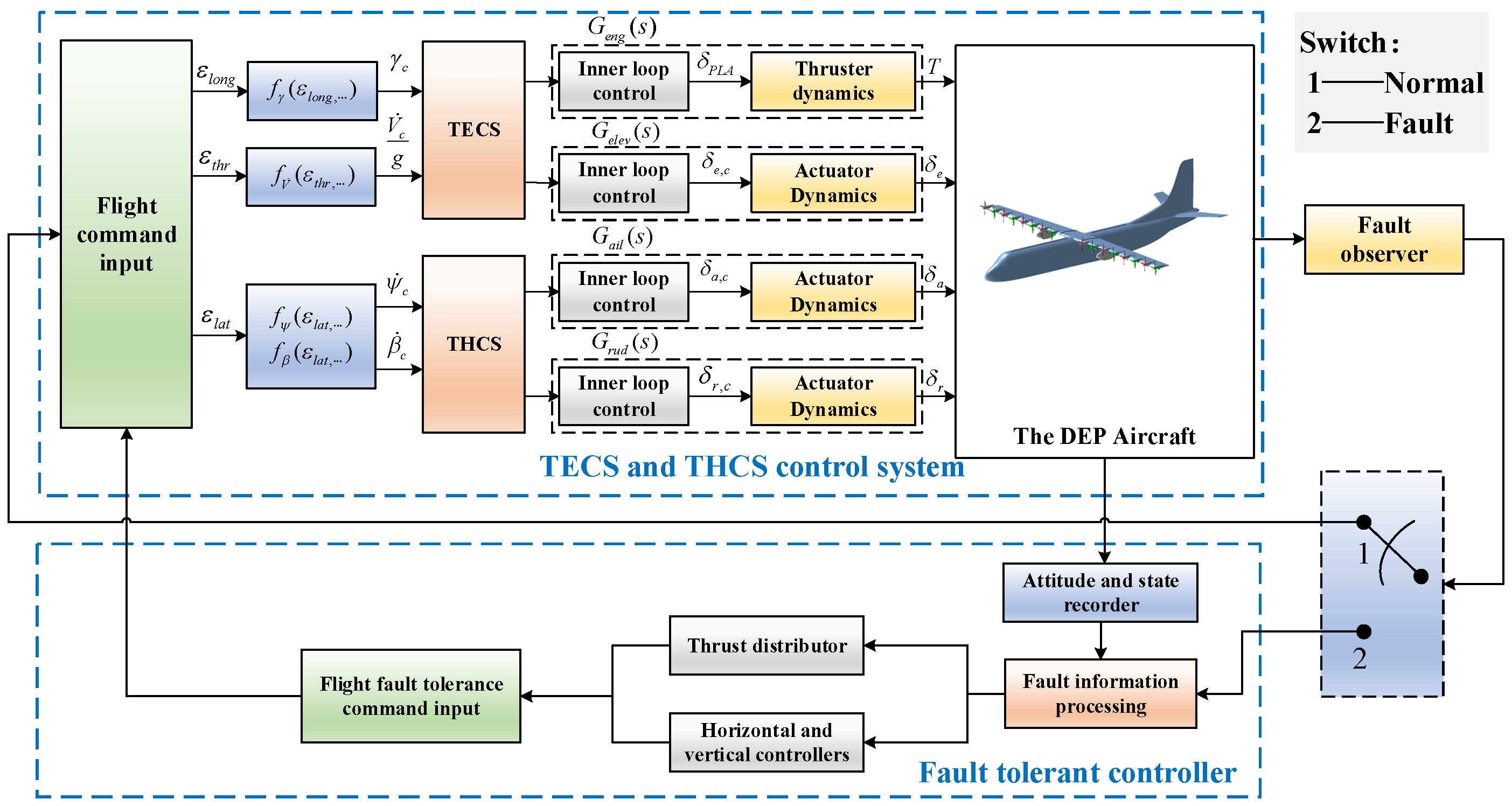
3. Coordinated Thrust Control and Fault-Tolerant Control of the DEP Aircraft

3.1. Coordinated Thrust Control of the DEP Aircraft

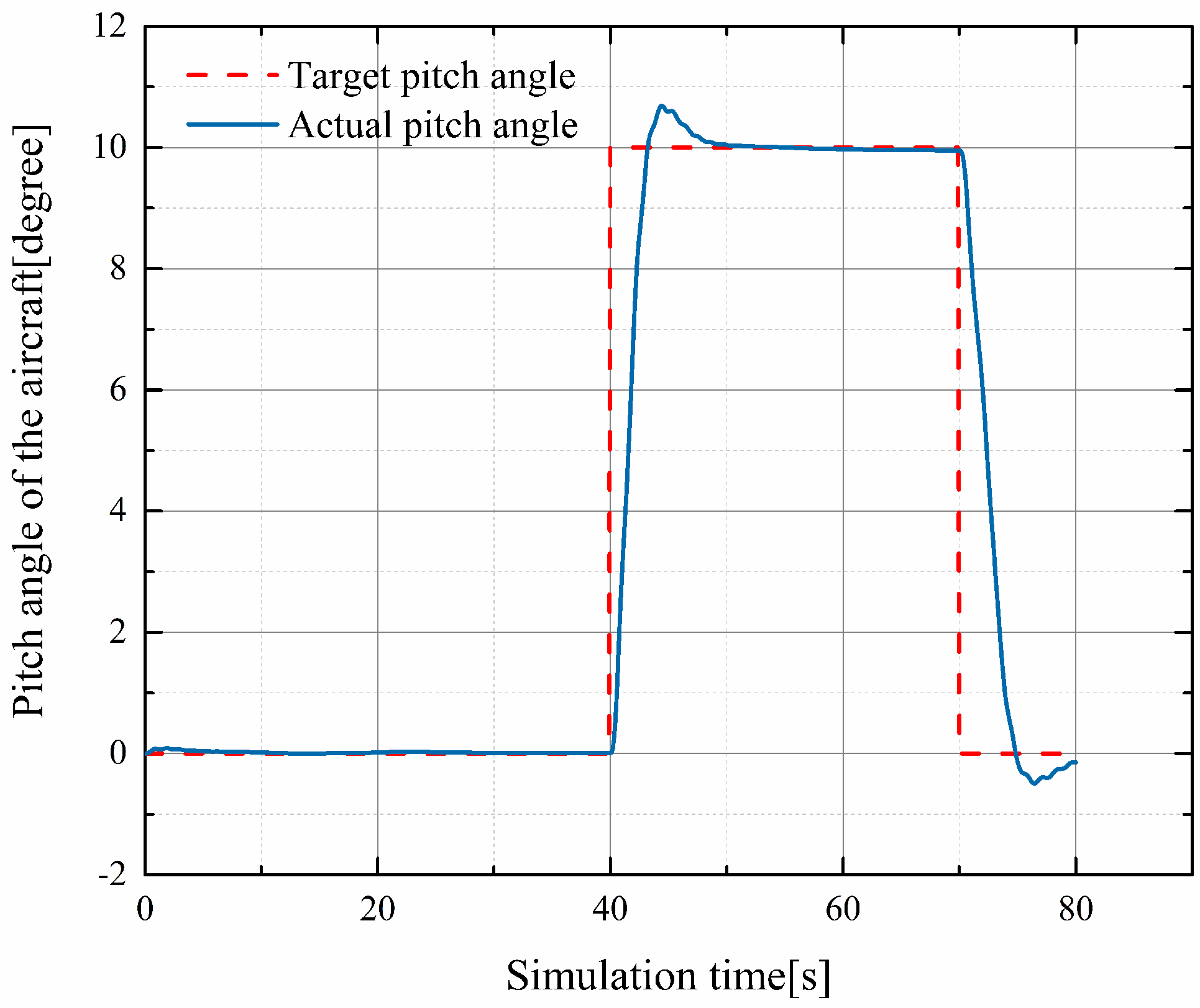
3.1.1. Longitudinal Control Loop

In this study, a total energy control system (TECS) was designed for the longitudinal control of DEP aircrafts, which controls the entire flight of climb, cruise and descent with the best goal of minimizing the aircraft’s energy consumption [24]. The system solves the coupling problems concerning the power lever angle and the elevator. Based on the total aircraft energy, the throttle directly corresponds to the increase or decrease in the overall aircraft energy, the rise and fall directly correspond to the distribution of the aircraft’s kinetic and potential energy, and the altitude and airspeed are the results produced by the joint action of the power lever angle and the elevator. TECS was derived as follows:

$$E_{tot}=E_{kin}+E_{pot}=\frac{1}{2}m{V}_a{}^2+mgH$$

(35)

$$\frac{{\dot{E}}_{tot}}{mg}=\frac{m{V}_a{\dot{V}}_a}{mg}+\frac{\dot{H}mg}{mg}=\frac{V_a{\dot{V}}_a}{g}+\dot{H}$$

(36)

$${\dot{E}}_{spec}=\frac{{\dot{E}}_{tot}}{mg{V}_a}=\frac{{\dot{V}}_a}{g}+\frac{\dot{H}}{V_a}=\frac{{\dot{V}}_a}{g}+\sin \gamma \approx \frac{{\dot{V}}_a}{g}+\gamma$$

(37)

$${\dot{E}}_{dist}=\gamma -\frac{{\dot{V}}_a}{g}$$

(38)

In the equations, $E_{tot}$ is the total energy of the aircraft, $E_{kin}$ is the kinetic energy of the aircraft, $E_{pot}$ is the potential energy of the aircraft, $m$ is the aircraft mass, $H$ is the altitude, $g$ is the gravitational acceleration, $V_a$ is the airspeed, $\gamma$ is the track angle, and ${\dot{E}}_{dist}$ is the specific energy distribution rate. In addition, the incremental thrust $\Delta T_c$ is associated with the specific energy gradient ${\dot{E}}_{spec}$.

The TECS approach connects the change in commanded thrust to the change in specific energy rate as follows:

$$\Delta T_c=\left(K_{TP}+\frac{K_{TI}}{s}\right){\dot{E}}_{spec}$$

(39)

In the above equation in $s$ domain, $K_{TP}$ is the proportional gain of the thrust control loop, while $K_{TI}$ is the integral gain of the thrust control loop that drives the steady-state error to zero. It was assumed that the elevator control is under energy conservation and the elevator can convert kinetic energy to potential energy, so the specific energy distribution rate is presented as follows:

$${\dot{E}}_{dist}=\gamma -\frac{{\dot{V}}_a}{g}$$

(40)

Based on that, changes in pitch angle command $\Delta {\theta }_c$ are related to changes in ${\dot{E}}_{dist}$:

$$\Delta {\theta }_c=\left(K_{EP}+\frac{K_{EI}}{s}\right){\dot{E}}_{dist}$$

(41)

where $K_{EP}$ is the proportional gain of the pitch angle control loop, and $K_{EI}$ is the integral gain of the pitch angle control loop.

The aircraft’s thrust is associated with the thrust command, and the change of elevator deflection angle $\Delta {\delta }_e$ is related to the pitch command:

$$\Delta T=G_{eng}\left(s\right)\Delta T_c,\Delta {\delta }_e=G_{elev}\left(s\right)\Delta {\theta }_c$$

(42)

where $G_{thr}(s)$ denotes the combined thrust control function, and $G_{elev}(s)$ is the combined pitch control and elevator actuator dynamics function. Based on the above derivation, the functional block diagram of TECS can be represented as in Figure 6.

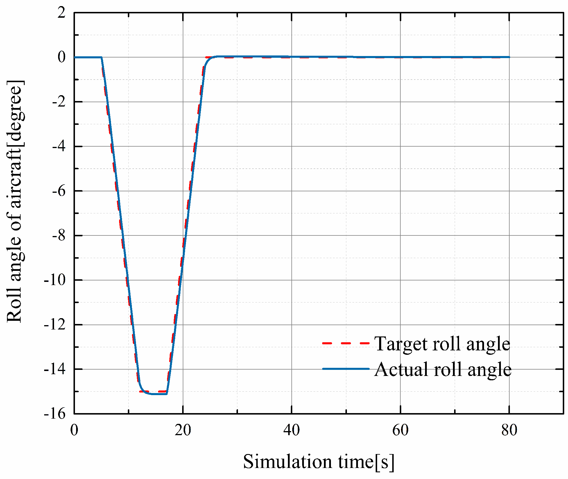
3.1.2. Lateral Control Loop

The total heading control system (THCS) is leveraged for the lateral control of DEP aircrafts [24]. The error signals between the commanded and actual rate of change of heading (${\dot{\psi }}_c$ and $\dot{\psi }$) and between the commanded and actual rate of change of sideslip (${\dot{\beta }}_c$ and $\dot{\beta }$) are computed as follows:

$$\Delta \dot{\psi }={\dot{\psi }}_c-\dot{\psi }$$

(43)

$$\Delta \dot{\beta }={\dot{\beta }}_c-\dot{\beta }$$

(44)

The commanded roll angle changes $\Delta {\varphi }_c$ and the yaw rate changes $\Delta r_c$ based on these errors are calculated as follows:

$$\Delta {\varphi }_c=\frac{V_a}{g}\left(K_{RP}+\frac{K_{RI}}{s}\right)\left(\Delta \dot{\psi }+\Delta \dot{\beta }\right)$$

(45)

$$\Delta r_c=\frac{V_a}{g}\left(K_{YP}+\frac{K_{YI}}{s}\right)\left(\Delta \dot{\psi }-\Delta \dot{\beta }\right)$$

(46)

where $K_{RP},K_{RI}$ is the proportional gain and integral gain of the roll angle control loop, and $K_{YP},K_{YI}$ is the proportional gain and integral gain of the yaw rate control loop.

In terms of aircraft-related components, deflection changes in ailerons $\Delta {\delta }_a$ and the deflection changes in rudder $\Delta {\delta }_r$ are calculated in response to roll angle commands and roll angle speed variations, respectively.

$$\Delta {\delta }_a=G_{ail}\left(s\right)\Delta {\varphi }_c,\Delta {\delta }_r=G_{rud}\left(s\right)\Delta r_c$$

(47)

where $G_{ail}(s)$ and $G_{rud}(s)$ are ailerons and the rudder controller and the actuator dynamics function, respectively.

3.2. Fault Response Strategy and Fault-Tolerant Control of DEP Aircrafts

This study focused on stuck and failed thrusters. Causes of thruster fault include decreased gain of a brushless motor due to aging of the motor stator coils, excessive friction of the motor rotor’s shaft, and degradation of the motor’s magnet performance, leading to the output deviating from the normal one. Macroscopically, when the output of a brushless motor is weak during the actual flight, changes in attitude angle of the motor is reduced with the same control amount, and the entire aircraft becomes “sluggish”. In this study, 16 electric thrusters were adopted for the model object, with a symmetric distribution of eight thrusters on the left and eight on the right. The thruster near the center was numbered 1, and the outermost thruster was numbered 8. The state matrices of the thrusters on the left and the right were expressed by $X_L$ and $X_R$. In the preliminary design, the total thrust of the system is given by Equation (50), assuming that the thrust of all thrusters on the same side is equal [25].

$$T_{R\_i}=T_{R\_j},\forall i\in [1,8],j\in [1,8]$$

(48)

$$T_{L\_i}=T_{L\_j},\forall i\in [1,8],j\in [1,8]$$

(49)

$$T_{total}=T_L\underset{i=1}{\overset{8}{\mathsf{\Sigma }}}{X}_L(i)+T_R\underset{i=1}{\overset{8}{\mathsf{\Sigma }}}{X}_R(i)$$

(50)

Through this thruster counting method, the total yaw moment provided by this propulsion system is given by Equation (51), where the diameter of each thruster is $D$:

$$M_{tot}=T_L\frac{D}{2}\underset{i=1}{\overset{8}{\mathsf{\Sigma }}}(2i-1)X_L(i)-T_R\frac{D}{2}\underset{i=1}{\overset{8}{\mathsf{\Sigma }}}(2i-1)X_R(i)$$

(51)

Solving $T_R$ in (50) and (51), $T_{Left}$ and $T_{Right}$ can be obtained as shown in Equations (53) and (54) below:

$$M_{tot}=T_L\frac{D}{2}\underset{i=1}{\overset{8}{\mathsf{\Sigma }}}(2i-1)X_L(i)-(\frac{T_{tot}}{\underset{i=1}{\overset{8}{\mathsf{\Sigma }}}{X}_R(i)}-\frac{\underset{i=1}{\overset{8}{\mathsf{\Sigma }}}{X}_L(i)}{\underset{i=1}{\overset{8}{\mathsf{\Sigma }}}{X}_R(i)})\frac{D}{2}\underset{i=1}{\overset{8}{\mathsf{\Sigma }}}(2i-1)X_R(i)$$

(52)

$$T_{Left}=\frac{\frac{2}{D}{M}_{tot}+\frac{T_{tot}}{\underset{i=1}{\overset{8}{\mathsf{\Sigma }}}{X}_R(i)}\underset{i=1}{\overset{8}{\mathsf{\Sigma }}}(2i-1)X_R(i)}{\underset{i=1}{\overset{8}{\mathsf{\Sigma }}}(2i-1)[X_L(i)]+\frac{\underset{i=1}{\overset{8}{\mathsf{\Sigma }}}{X}_L(i)}{\underset{i=1}{\overset{8}{\mathsf{\Sigma }}}{X}_R(i)}\underset{i=1}{\overset{8}{\mathsf{\Sigma }}}(2i-1)[X_R(i)]}$$

(53)

$$T_{Right}=\frac{T_{tot}}{\underset{i=1}{\overset{8}{\mathsf{\Sigma }}}{X}_R(i)}-\frac{\frac{2}{D}{M}_{tot}+\frac{T_{tot}}{\underset{i=1}{\overset{8}{\mathsf{\Sigma }}}{X}_R(i)}\underset{i=1}{\overset{8}{\mathsf{\Sigma }}}(2i-1)X_R(i)}{\frac{\underset{i=1}{\overset{8}{\mathsf{\Sigma }}}{X}_R(i)}{\underset{i=1}{\overset{8}{\mathsf{\Sigma }}}{X}_L(i)}\underset{i=1}{\overset{8}{\mathsf{\Sigma }}}(2i-1)[X_L(i)]+\underset{i=1}{\overset{8}{\mathsf{\Sigma }}}(2i-1)[X_R(i)]}$$

(54)

$T_{Left}$ and $T_{Right}$ of the above equations were input as thrust commands to the electric thrusters on both sides, where the state matrices of the thrusters were considered for monitoring the minimum thrust demand, turbine engine state, generator state, power bus state, and electric thruster state. If any of the components fail, the corresponding variable in the state matrices degrades to 0. In addition to enabling coordinated control of the electric thrusters on both sides, the thrust can be redistributed to maintain stability and maneuverability of the aircraft in case of a component fault. The fault-tolerant controller of the DEP system designed in this study features a fault injection module. The function developed so far allows the remaining thrusters to make corresponding changes to recover the aircraft’s thrust to the prefault level when a single thruster on the left/right fails and the torque and the rotational speed fail to reach the normal operational level.

When the $i$th thruster fails, the mathematical form of the rotational speed of the thruster can be expressed as follows:

$${\omega }_i^f={\sigma }_i{\omega }_i$$

(55)

where $0\le {\sigma }_i<1$ denotes the fault rate of the $i$th thruster under a fault. When the motor is completely jammed, then ${\sigma }_i=0$.

When a simulation test of thruster fault-tolerant control is conducted in this simulation platform, a random fault thruster ID number, that is $n_{Fault}$, will be randomly generated in the $\tau$th second in order to simulate a thruster fault more realistically.

When a thruster numbered $n_{Fault}$ fails in the $\tau$th second, the torque of the thruster corresponding to the failed thruster should be first controlled to the torque value of the failed one, i.e., $T_i\ast {\sigma }_i$, at which point the difference between the thrust in a steady-state flight and that of a failed aircraft is deemed as the control error ${\psi }_{err}$. In this case, the thruster control torque needed to recover the prefault thrust can be calculated by PID control, which will be fed back to the aircraft control input, in order to achieve the fault-tolerant control of thrusters in the DEP system. The functional block diagram of the designed fault-tolerant control methods for DEP aircrafts in this study is shown in Figure 7.

4. Simulation Results and Discussion

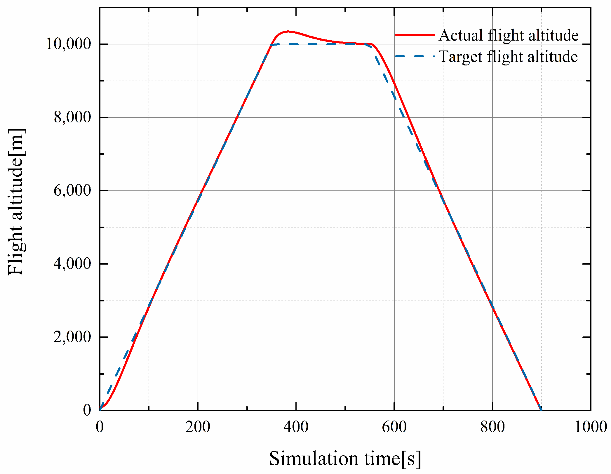
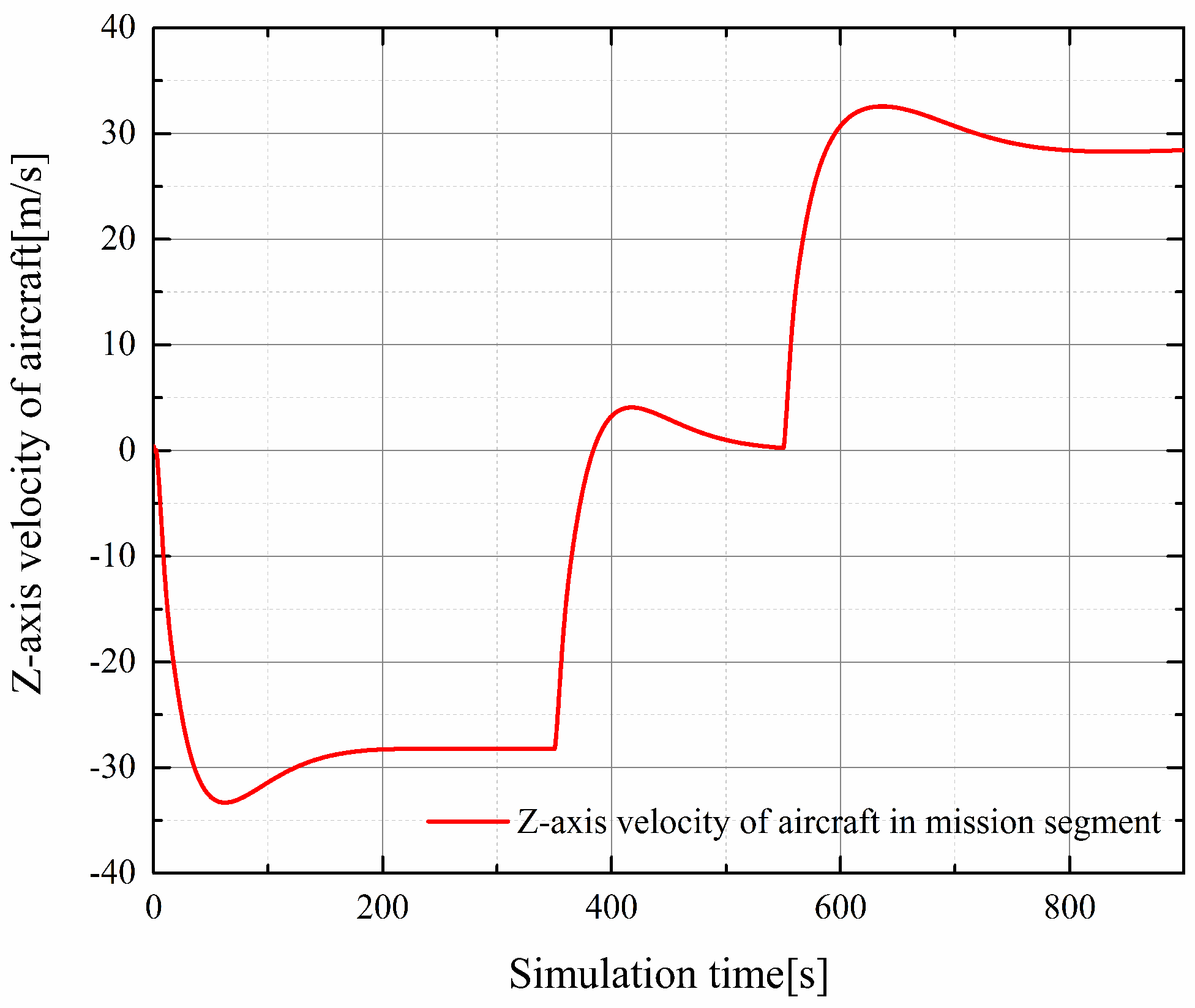
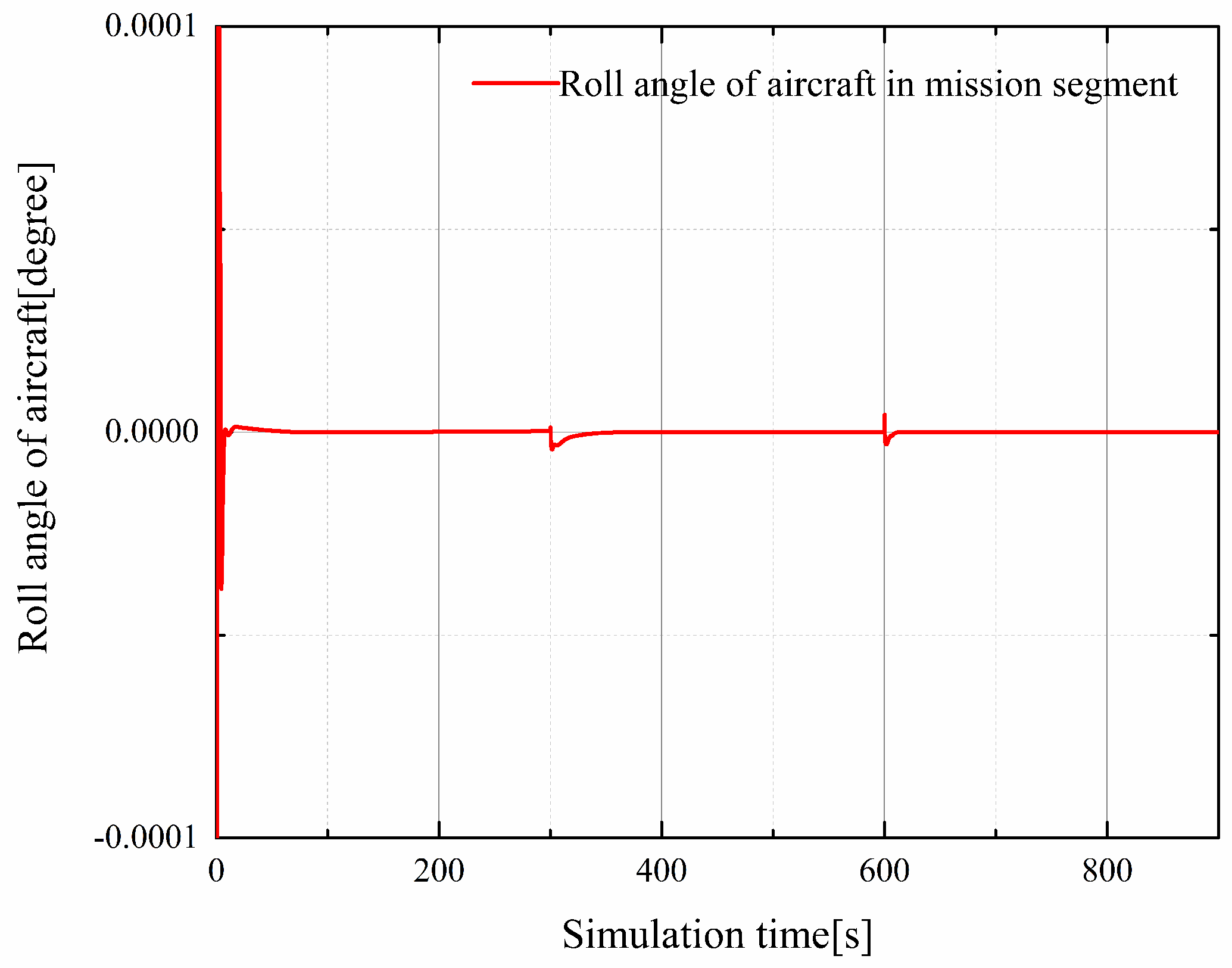
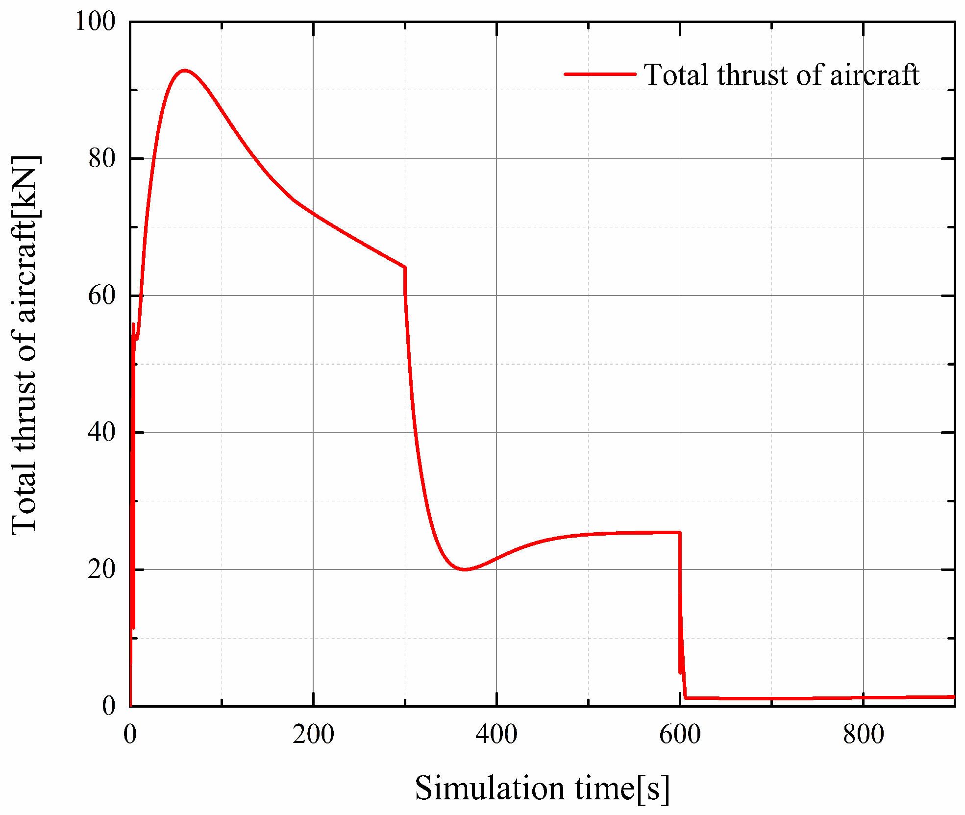
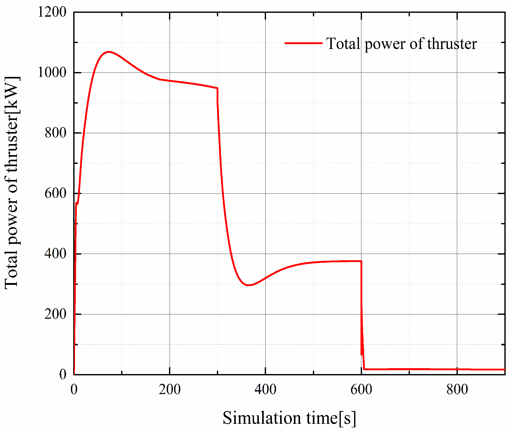
4.1. Simulation Tests Carried out within Mission Segments

Simulation tests of the DEP aircraft on the coordinated and comprehensive control of thrust were conducted during the entire process in the mission profile, namely takeoff, cruise, and descent. The set flight conditions are shown in

Table 1. Parameter setting in mission segments of takeoff/cruise/descent.

Flight Phase	Starting Height (m)	Final Height (m)	Mach Number
Climb	0	10,000	0.49
Cruise	10,000	10,000	0.79
Descent	10,000	0	0.18

.

The flight simulation test results of the control system within the full mission segments are presented in Figure 8, with the response curve of the flight altitude showing good tracking effects.

For the altitude control within the flight mission segment, the quantitative description of the control effect is shown in

Table 2. The performance index of DEP aircraft’s altitude control.

Performance Index	Value	Unit
Rise time	349.75	seconds
Peak time	375.97	seconds
Settling time	493.61	seconds
Overshoot	3.46	percent

, including rise time, peak time, settling time, and overshoot.

Figure 9 is the acceleration response curve of the z-axis. As can be seen, there is a change of acceleration when the aircraft’s flight state changes. The curve then converges to zero. Figure 10 is the velocity response curve of the z-axis. When the aircraft enters cruise from climb, changes in acceleration results in the aircraft’s velocity in the z-axis reaching almost zero in order to maintain a flight state with constant height and uniform speed.

Variation trend of the pitch angle of the aircraft in the corresponding mission segments is shown in Figure 11. During the cruise phase, the pitch angle of the aircraft returns to zero degrees.

Figure 12 and Figure 13 show the variation trend of the roll angle and yaw angle of an aircraft in the corresponding mission segments. The roll angle and the yaw angle will witness some small changes at the moment the flight state switches due to changes in the thrust and the attitude of thrusters in the DEP system. They will then return to a flight state without roll and deviation. The test results verifies the stability of the control system designed in this study.

The thrust controller solves the control input torque of a corresponding single thruster to produce thrust in different stages. The curve of the total thrust variations generated by all thrusters in different mission segments is displayed in Figure 14. When the aircraft enters cruise in 300 s, the thrust required by the aircraft decreases, and the thrust is further reduced after it descends. The total power generated by the thruster module in the entire mission segments is demonstrated in Figure 15.

4.2. DEP System Thruster Fault-Tolerant Control Simulation Test

Propellers of thrusters on the left and right wings of an aircraft are designed to be right-handed and left-handed, and the torque direction is also symmetrical. When a thruster fails when $n_{Fault}=2$ and ${\sigma }_i=0.2$ is randomly generated at the 200th second, the torque of the failed thruster instantly drops to the moment value of $T_i\ast {\sigma }_i$, as shown by the red curve in Figure 16. Therefore, the torque of the symmetrical thruster No. 15 should change symmetrically in order to first ensure the balance of moment, as shown by the blue curve in Figure 16.

In order to recover a stable flight state, all thrusters, except the thrusters symmetrical to the failed ones, should increase their thrust, so the torque input of the rest thrusters should be up. As the remaining thrusters change in the same way, the response value of the thruster torque can be observed with thruster No. 1 as an example, and the input control torque of thruster No. 1 gradually increases after the fault occurs in the 200th second. The generated thrust also grows at the 200th second, as shown in Figure 17.

The variation curve of the total thrust of the DEP aircraft after the fault is shown in Figure 18. As can be seen, the total thrust decreases after the thruster fault occurs in the 200th second, and the thrust of each thruster on the left and right is then altered by coordinate control to recover the thrust to a level that can maintain a stable flight of the aircraft.

The controller can better control the thrust to the prefault level without overshoot after the total thrust changes in the 200th second, taking 0.3 s for adjustment. In other words, thrust generated by the thrusters on the left and right wing of the aircraft is evenly distributed by coordinated control after the fault.

5. Conclusions

First, a mathematical model of the DEP aircraft’s propulsion system, including the engine module, the generator and energy storage system module, and the thruster module, was established. Then, a mathematical model of the six-degree-of-freedom DEP aircraft was built based on the principles of aerodynamics and flight dynamics, which laid a theoretical foundation for subsequent simulation experiment.

Research on control methods to coordinate thrust from multiple thrusters were carried out based on the mathematical model of DEP aircrafts. The lateral and longitudinal control loops of DEP aircrafts were set up based on the principles of total energy and total heading control, and a simulation experiment was carried out in the mission segment of the DEP aircraft. The effects of aircraft attitude control and altitude control verified the stability and accuracy of the mathematical model of the aircraft.

Furthermore, a fault-tolerant control method was developed for the case where a thruster of a DEP aircraft has failed. Experiments simulating flight tests and fault-tolerant control within the mission segment were conducted, and the experimental results verified the effectiveness of the designed coordinated thrust control system and the fault-tolerant control method. The controller could control the thrust to the prefault level.

The correctness and effectiveness of the designed coordinated thrust control method and fault-tolerant control method for DEP aircrafts were theoretically verified, providing a theoretical basis for future engineering application and development of the control system for DEP aircrafts.

References

1. Serrano, J.R.; García-Cuevas, L.M.; Bares, P.; Varela, P. Propeller Position Effects over the Pressure and Friction Coefficients over the Wing of an UAV with Distributed Electric Propulsion: A Proper Orthogonal Decomposition Analysis. Drones 2022, 6, 38. [Google Scholar] [CrossRef]
2. Amoozgar, M.; Friswell, M.; Fazelzadeh, S.; Khodaparast, H.H.; Mazidi, A.; Cooper, J. Aeroelastic Stability Analysis of Electric Aircraft Wings with Distributed Electric Propulsors. Aerospace 2021, 8, 100. [Google Scholar] [CrossRef]
3. Serrano, J.; Tiseira, A.; García-Cuevas, L.; Varela, P. Computational Study of the Propeller Position Effects in Wing-Mounted, Distributed Electric Propulsion with Boundary Layer Ingestion in a 25 kg Remotely Piloted Aircraft. Drones 2021, 5, 56. [Google Scholar] [CrossRef]
4. Kirner, R.; Raffaelli, L.; Rolt, A.; Laskaridis, P.; Doulgeris, G.; Singh, R. An assessment of distributed propulsion: Part B – Advanced propulsion system architectures for blended wing body aircraft configurations. Aerosp. Sci. Technol. 2016, 50, 212–219. [Google Scholar] [CrossRef]
5. Gohardani, A.S.; Doulgeris, G.; Singh, R. Challenges of future aircraft propulsion: A review of distributed propulsion technology and its potential application for the all electric commercial aircraft. Prog. Aerosp. Sci. 2011, 47, 369–391. [Google Scholar] [CrossRef]
6. Nickol, C.L.; Haller, W.J. Assessment of the Performance Potential of Advanced Subsonic Transport Concepts for NASA’s Environmentally Responsible Aviation Project. In Proceedings of the 54th AIAA Aerospace Sciences Meeting, San Diego, CA, USA, 4–8 January 2016; p. 1030. [Google Scholar]
7. Connolly, J.W.; Chapman, J.W.; Stalcup, E.J.; Chicatelli, A.; Hunker, K.R. Modeling and Control Design for a Turboelectric Single Aisle Aircraft Propulsion System. In Proceedings of the 2018 AIAA/IEEE Electric Aircraft Technologies Symposium (EATS), Cincinnati, OH, USA, 12–14 July 2018; pp. 1–19. [Google Scholar]
8. Nguyen, N.T.; Reynolds, K.; Ting, E.; Nguyen, N. Distributed Propulsion Aircraft with Aeroelastic Wing Shaping Control for Improved Aerodynamic Efficiency. J. Aircr. 2018, 55, 1122–1140. [Google Scholar] [CrossRef]
9. Zhang, J.; Kang, W.; Li, A.; Yang, L. Integrated flight/propulsion optimal control for DPC aircraft based on the GA-RPS algorithm. Proc. Inst. Mech. Eng. Part G J. Aerosp. Eng. 2015, 230, 157–171. [Google Scholar] [CrossRef]
10. Lei, T.; Kong, D.; Wang, R.; Li, W.; Zhang, X. Evaluation and optimization method for power systems of distributed electric propulsion aircraft. Acta Aeronaut. Et Astronaut. Sin. 2021, 42, 624047. (In Chinese) [Google Scholar] [CrossRef]
11. Da, X.; Fan, Z.; Xiong, N.; Wu, J.; Zhao, Z. Modeling and analysis of distributed boundary layer ingesting propulsion system. Acta Aeronaut. Et Astronaut. Sin. 2018, 39, 122048. (In Chinese) [Google Scholar] [CrossRef]
12. Liu, C.; Si, X.; Teng, J.; Ihiabe, D. Method to Explore the Design Space of a Turbo-Electric Distributed Propulsion System. J. Aerosp. Eng. 2016, 29, 04016027. [Google Scholar] [CrossRef]
13. Choi, B.; Brown, G.V.; Morrison, C.; Dever, T. Propulsion Electric Grid Simulator (PEGS) for Future Turboelectric Distributed Propulsion Aircraft. In Proceedings of the 12th International Energy Conversion Engineering Conference, Cleveland, OH, USA, 28–30 July 2014; p. 3644. [Google Scholar]
14. Rothhaar, P.M.; Murphy, P.C.; Bacon, B.J.; Gregory, I.M.; Grauer, J.A.; Busan, R.C.; Croom, M.A. NASA Langley Distributed Propulsion VTOL TiltWing Aircraft Testing, Modeling, Simulation, Control, and Flight Test Development. In Proceedings of the 14th AIAA Aviation Technology, Integration, and Operations Conference, Atlanta, GA, USA, 16–20 June 2014; p. 2999. [Google Scholar] [CrossRef] [Green Version]
15. Freeman, J.L.; Klunk, G.T. Dynamic Flight Simulation of Spanwise Distributed Electric Propulsion for Directional Control Authority. In Proceedings of the 2018 AIAA/IEEE Electric Aircraft Technologies Symposium, Cincinnati, OH, USA, 9–11 July 2018; Volume 2018, pp. 1–15. [Google Scholar] [CrossRef]
16. Kratz, J.L.; Thomas, G.L. Dynamic Analysis of the STARC-ABL Propulsion System. In Proceedings of the AIAA Propulsion and Energy 2019 Forum, Indianapolis, IN, USA, 19–22 August 2019. [Google Scholar]
17. Van, E.N.; Alazard, D.; Döll, C.; Pastor, P. Co-design of aircraft vertical tail and control laws using distributed electric propulsion. IFAC-Pap. 2019, 52, 514–519. [Google Scholar] [CrossRef]
18. Van, E.N.; Alazard, D.; Döll, C.; Pastor, P. Co-design of aircraft vertical tail and control laws with distributed electric propulsion and flight envelop constraints. CEAS Aeronaut. J. 2021, 12, 101–113. [Google Scholar] [CrossRef]
19. Garrett, M.; Avanesian, D.; Granger, M.; Kowalewski, S.; Maroli, J.; Miller, W.A.; Jansen, R.; Kascak, P.E. Development of an 11 kW lightweight, high efficiency motor controller for NASA X-57 Distributed Electric Propulsion using SiC MOSFET Switches. In Proceedings of the AIAA (American Institute of Aeronautics and Astronautics) Propulsion and Energy 2019 Forum, Indianapolis, IN, USA, 19–22 August 2019; pp. 1–8. [Google Scholar]
20. Klunk, G.T.; Freeman, J.L. Vertical Tail Area Reduction for Aircraft with Spanwise Distributed Electric Propulsion. In Proceedings of the 2018 AIAA/IEEE Electric Aircraft Technologies Symposium, Cincinnati, OH, USA, 9–11 July 2018; p. 5022. [Google Scholar] [CrossRef]
21. Suzuki, Y.; Dunham, W.; Kolmanovsky, I.; Girard, A. Failure Detection and Control of Distributed Electric Propulsion Aircraft Engines. In Proceedings of the AIAA Scitech 2019 Forum, San Diego, CA, USA, 7–11 January 2019; p. 0109. [Google Scholar]
22. Shah, R.; Sands, T. Comparing Methods of DC Motor Control for UUVs. Appl. Sci. 2021, 11, 4972. [Google Scholar] [CrossRef]
23. Koo, S.M.; Travis, H.D.; Sands, T. Evaluation of Adaptive and Learning in Unmanned Systems. Preprints 2022. [Google Scholar] [CrossRef]
24. Chakraborty, I.; Ahuja, V.; Comer, A.; Mulekar, O. Development of a Modeling, Flight Simulation, and Control Analysis Capability for Novel Vehicle Configurations. In Proceedings of the AIAA Aviation 2019 Forum, Dallas, TX, USA, 17–21 June 2019; p. 3112. [Google Scholar]
25. Armstrong, M.; Ross, C.; Phillips, D.; Blackwelder, M. Stability, Transient Response, Control, and Safety of a High-Power Electric Grid for Tur-Boelectric Propulsion of Aircraft; NASA/CR 2013-217865; National Aeronautics and Space Administration: Cleveland, OH, USA, 2013.
Figure 1. The DEP aircraft studied in this paper.
Drones 06 00078 g001
Figure 2. Definition of ports of the electric power generation and energy storage system.
Drones 06 00078 g002
Figure 3. The pitch angle response of the DEP aircraft.
Drones 06 00078 g003
Figure 4. The roll angle response of the DEP aircraft.
Drones 06 00078 g004
Figure 5. The sideslip angle response of the DEP aircraft.
Drones 06 00078 g005
Figure 6. Functional block diagram of TECS.
Drones 06 00078 g006
Figure 7. Functional block diagram of the fault-tolerant control of the DEP aircraft.
Drones 06 00078 g007
Figure 8. Response curve of the flight altitude.
Drones 06 00078 g008
Figure 9. Acceleration response curve of the z-axis.
Drones 06 00078 g009
Figure 10. Velocity response curve of the z-axis.
Drones 06 00078 g010
Figure 11. Variation trend of the pitch angle in the mission segment.
Drones 06 00078 g011
Figure 12. Variation trend of the roll angle in the mission segment.
Drones 06 00078 g012
Figure 13. Variation trend of the yaw angle in the mission segment.
Drones 06 00078 g013
Figure 14. Curve of the total thrust variations generated by the thruster module.
Drones 06 00078 g014
Figure 15. Curve of the total power variations generated by the thruster module.
Drones 06 00078 g015
Figure 16. Variation curve of torque of the faulty thruster and symmetrical thruster.
Drones 06 00078 g016
Figure 17. Variation curve of the remaining normal thrusters with thruster No. 1 as an example.
Drones 06 00078 g017
Figure 18. Total thrust curve of the DEP aircraft after thruster fault.
Drones 06 00078 g018