
High-Temporal-Resolution Forest Growth Monitoring Based on Segmented 3D Canopy Surface from UAV Aerial Photogrammetry


Abstract
:1. Introduction
2. Materials and Methods
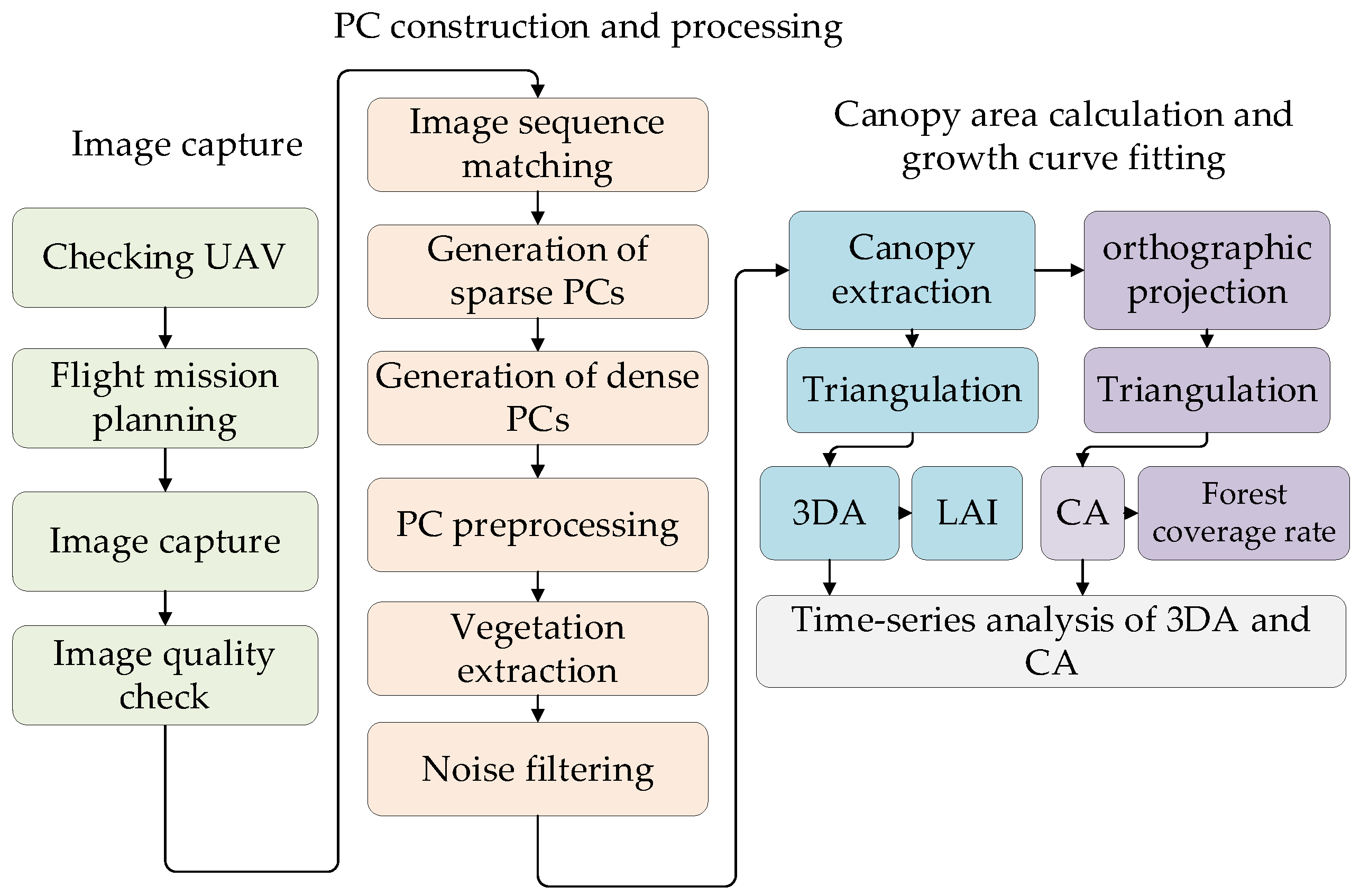
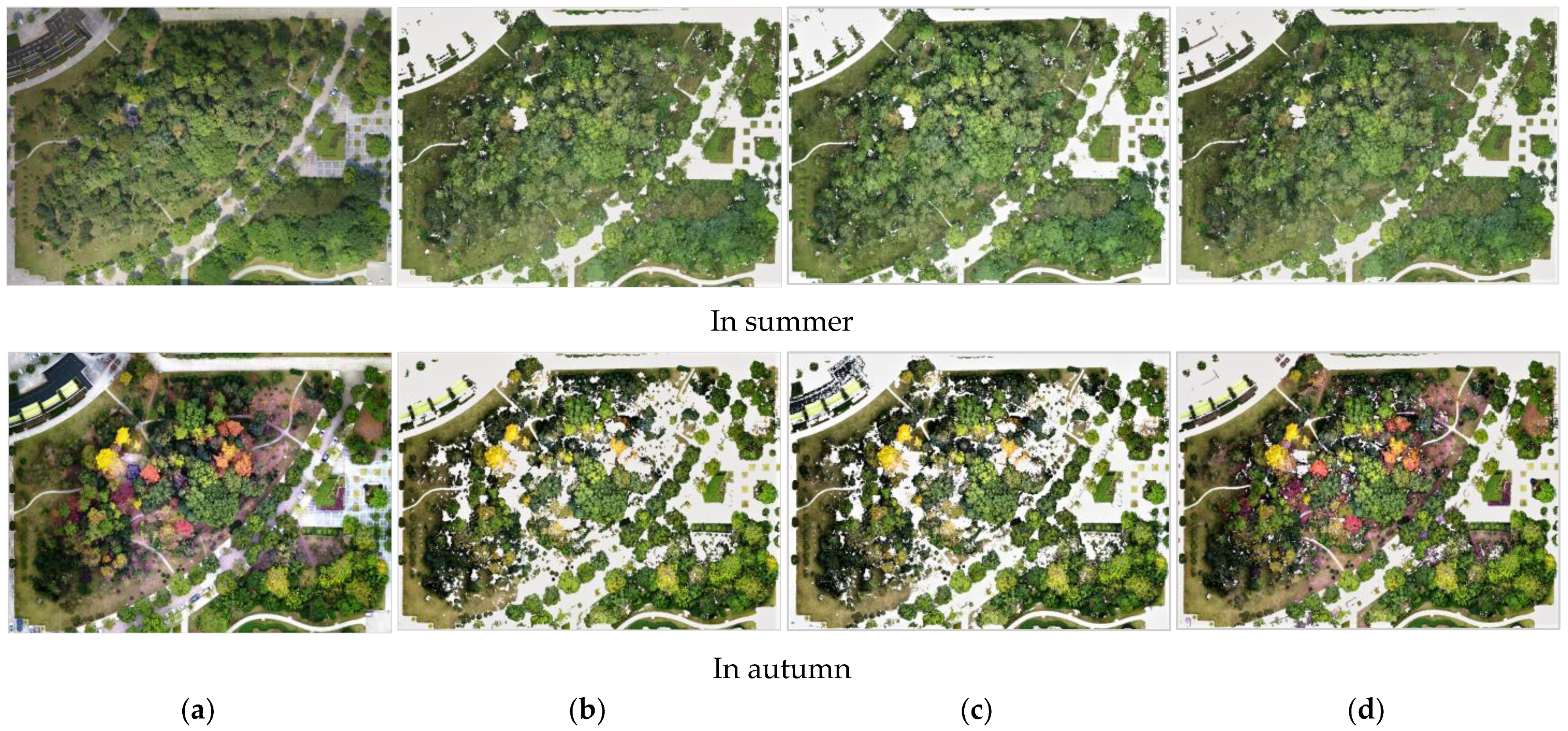
2.1. Remote Sensing Image Capture and 3D PCs Reconstruction
2.1.1. Remote Sensing Image Capturing
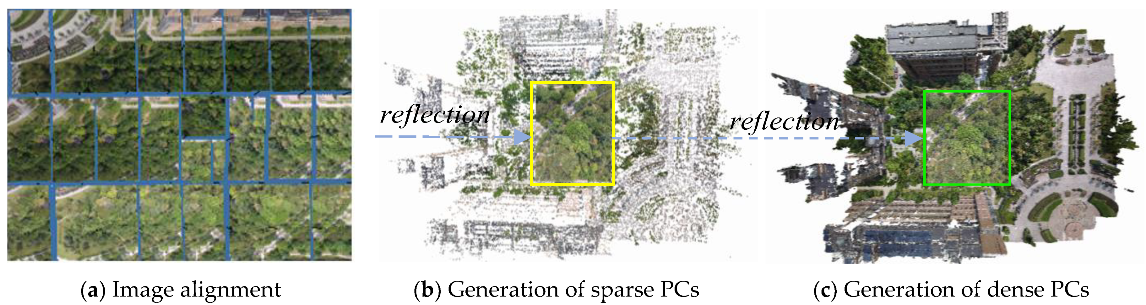
2.1.2. Three-Dimensional PC Construction and Preprocessing
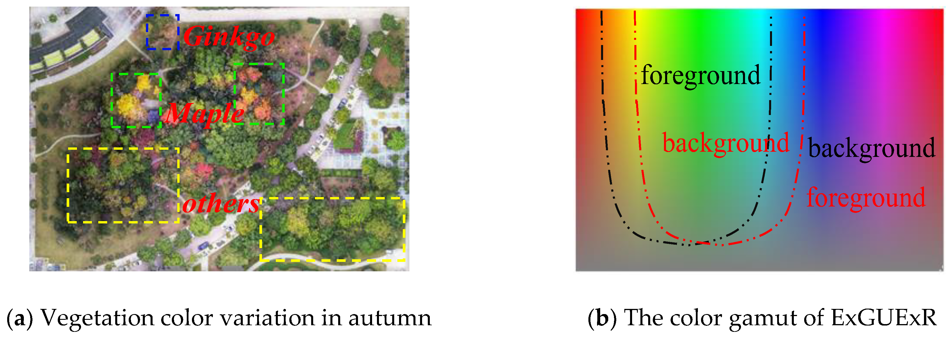
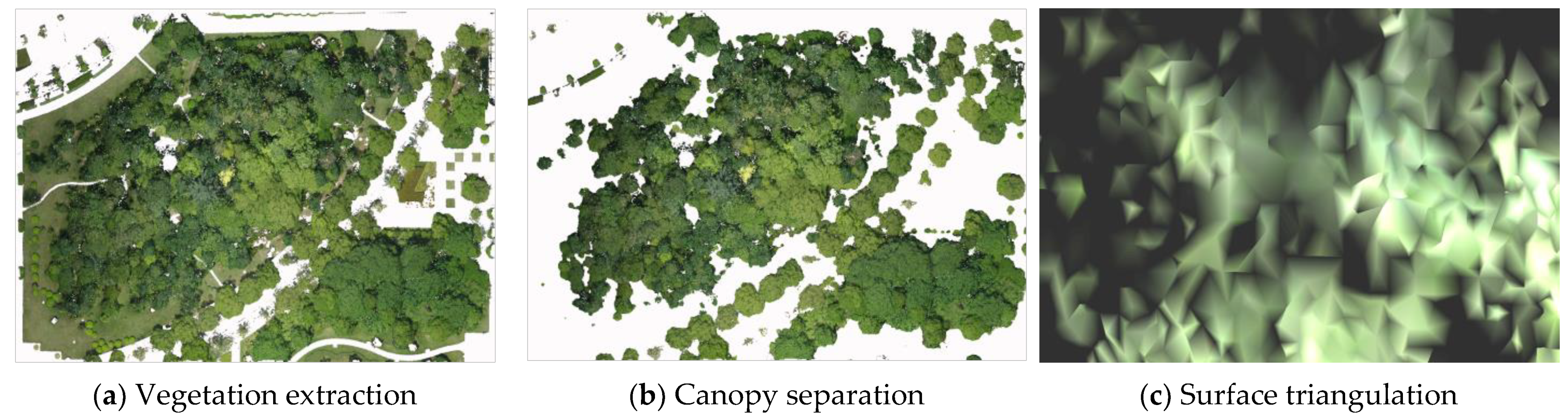
2.2. Vegetation Extraction and Filtering Noise
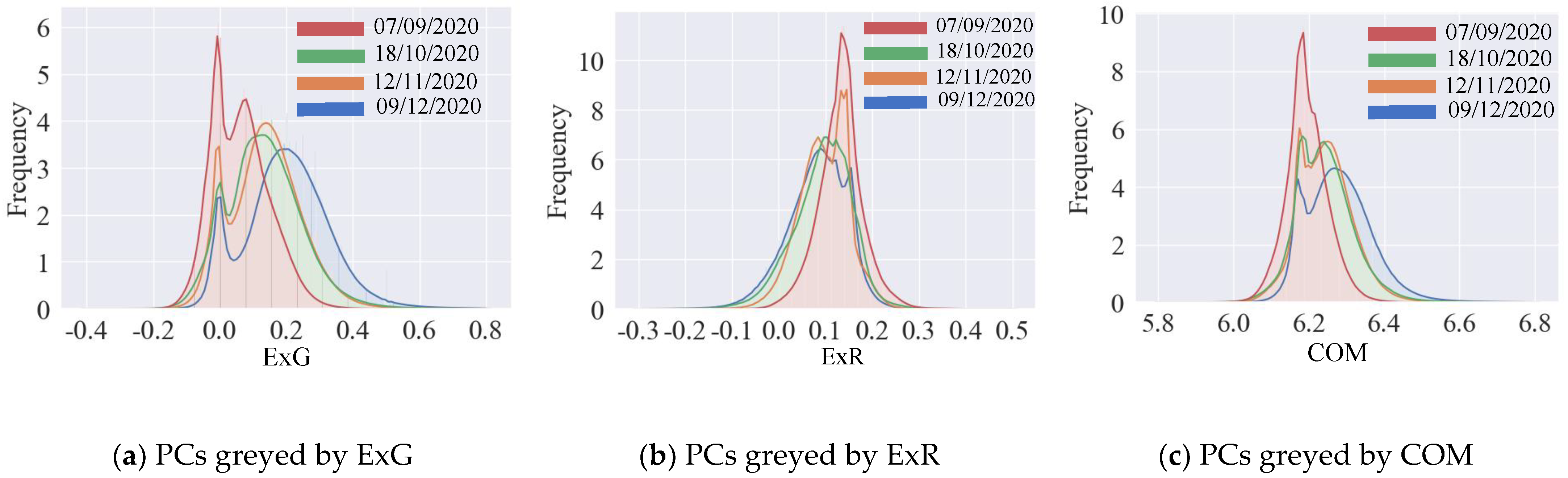
2.2.1. Spectral Vegetation Indices (SVIs)
- Excess green vegetation index (ExG)
- Combination of green indices (COM)
- Excess green union excess red index (ExGUExR)
2.2.2. Threshold Selection of SVIs and Filtered PCs
2.3. Separation Canopy from the Ground
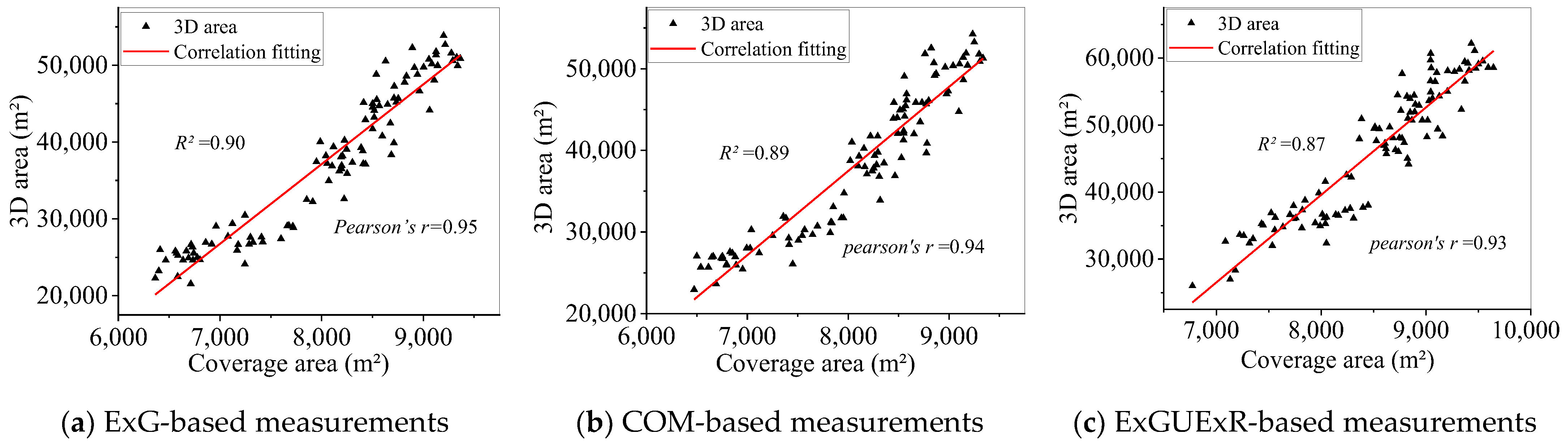
2.4. PCs Triangulation and Canopy 3D Area Measuring
2.5. Forest Canopy Coverage Area and Leaf Area Index (LAI)
2.6. Logistic Regression
3. Results and Analysis
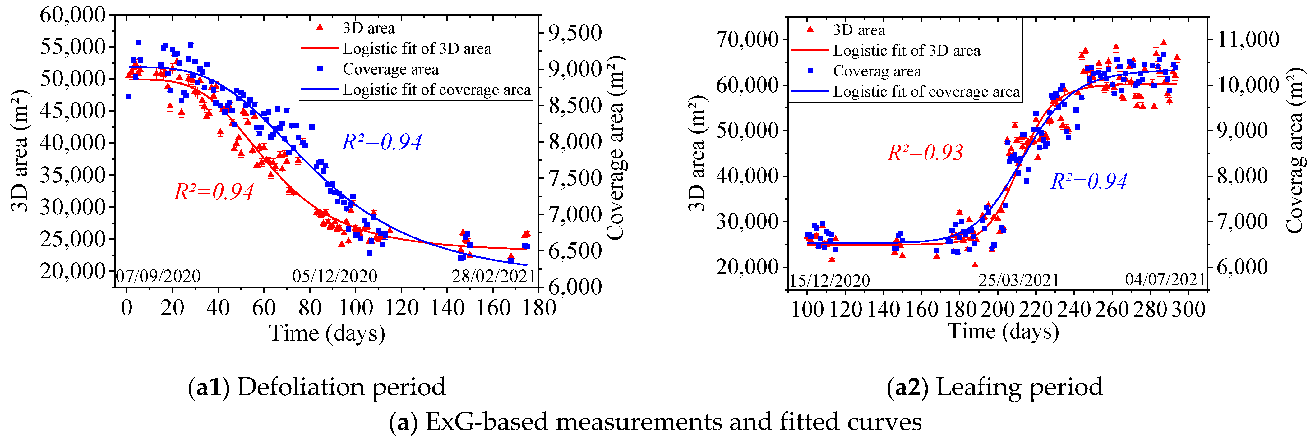
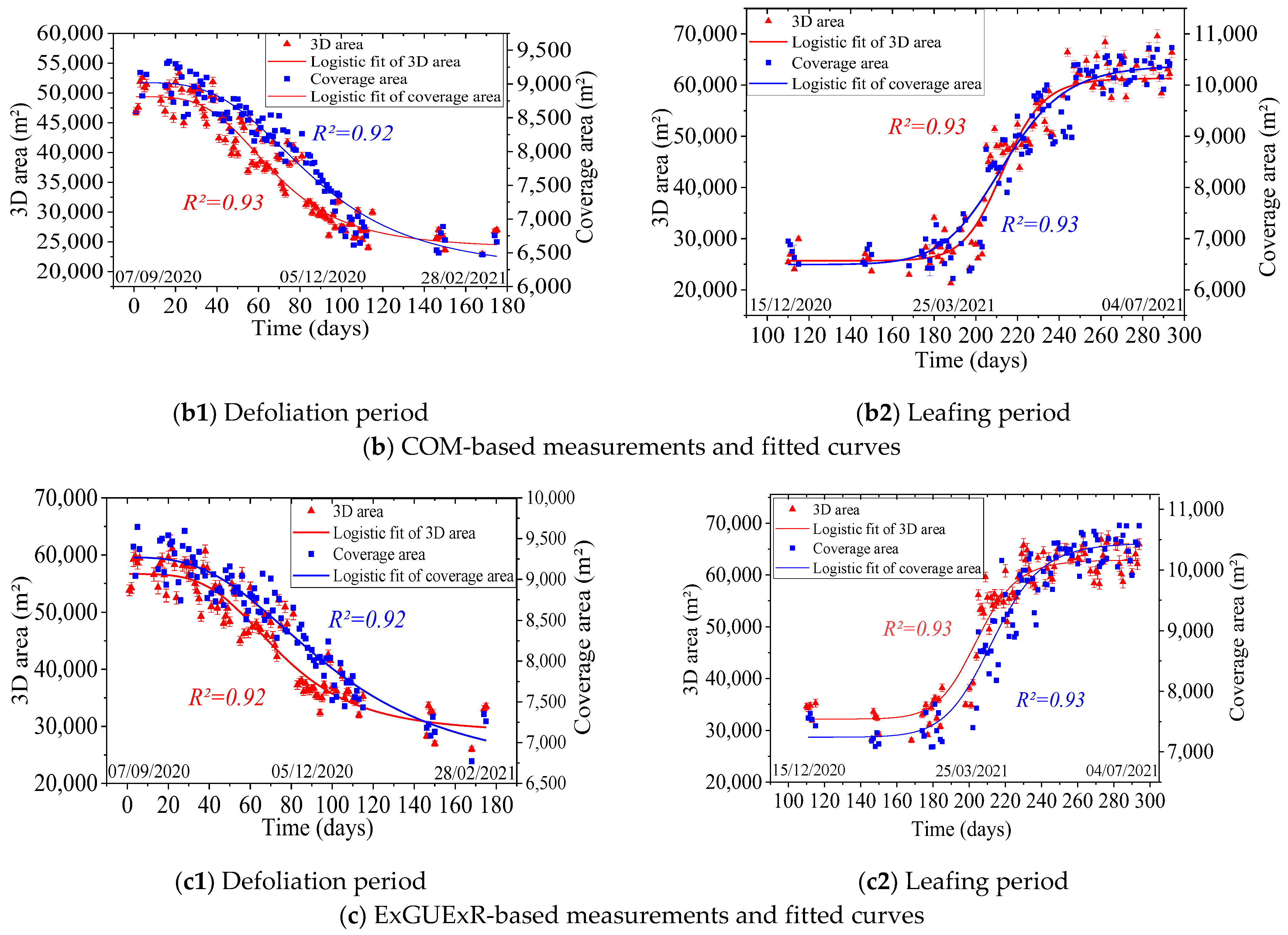
3.1. Canopy Area and Time-Series Analyses
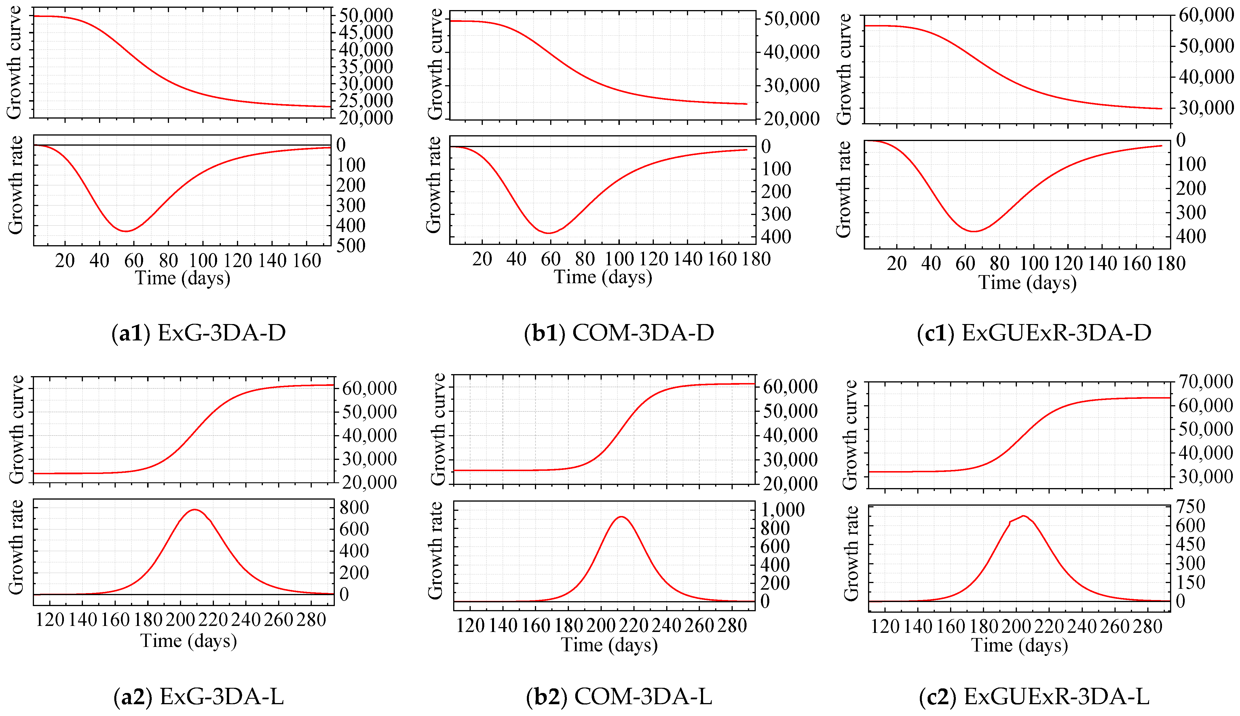
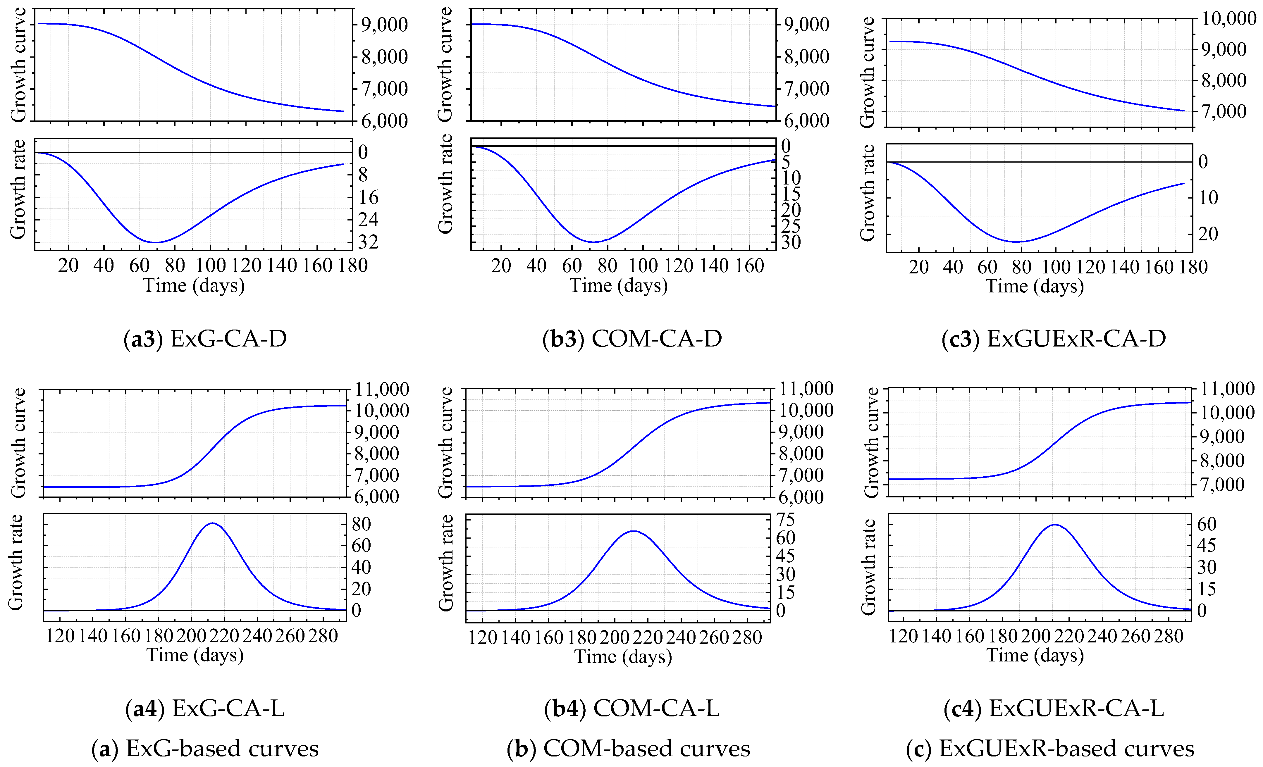
3.2. Canopy Growth Curve and Growth Rate Curve Analysis
3.2.1. General Growth Analysis Based on the Growth Curves and Rate Curves
3.2.2. Comparison of SVI-Extracted Vegetation and Their Curves
3.2.3. Comparison between 3DA and CA Curves
3.2.4. Calculation of Forest Coverage Rate and LAI
4. Discussion
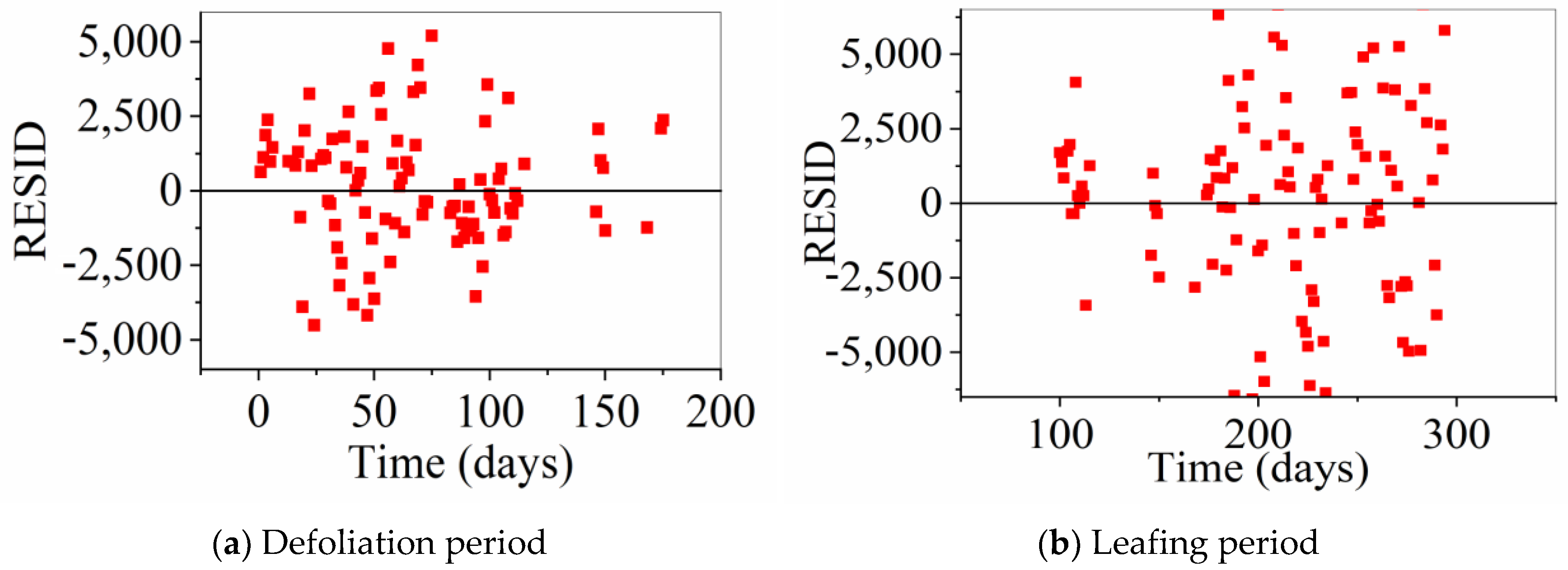
4.1. Error Analysis
4.1.1. Error Source Analysis
4.1.2. Analysis of Random Errors in Measurements
4.2. Comparison with Other Studies
4.3. The Applicability of the Proposed Method in Natural Forests
5. Conclusions
Author Contributions
Funding
Data Availability Statement
Conflicts of Interest
References
- Banskota, A.; Kayastha, N.; Falkowski, M.J.; Wulder, M.A.; Froese, R.E.; White, J.C. Forest monitoring using Landsat time series data: A review. Can. J. Remote Sens. 2014, 40, 362–384. [Google Scholar] [CrossRef]
- Wu, L.; Li, Z.; Liu, X.; Zhu, L.; Tang, Y.; Zhang, B.; Xu, B.; Liu, M.; Meng, Y.; Liu, B. Multi-Type Forest Change Detection Using BFAST and Monthly Landsat Time Series for Monitoring Spatiotemporal Dynamics of Forests in Subtropical Wetland. Remote Sens. 2020, 12, 341. [Google Scholar] [CrossRef] [Green Version]
- Bai, B.; Tan, Y.; Guo, D.; Xu, B. Dynamic Monitoring of Forest Land in Fuling District Based on Multi-Source Time Series Remote Sensing Images. ISPRS Int. J. Geo-Inf. 2019, 8, 36. [Google Scholar] [CrossRef] [Green Version]
- LANDSAT 9. Available online: https://landsat.gsfc.nasa.gov/satellites/landsat-9/ (accessed on 22 March 2022).
- Long, T.; Zhang, Z.; He, G.; Jiao, W.; Tang, C.; Wu, B.; Zhang, X.; Wang, G.; Yin, R. 30 m resolution global annual burned area mapping based on Landsat Images and Google Earth Engine. Remote Sens. 2019, 11, 489. [Google Scholar] [CrossRef] [Green Version]
- Walther, S.; Guanter, L.; Heim, B.; Jung, M.; Duveiller, G.; Wolanin, A.; Sachs, T. Assessing the dynamics of vegetation productivity in circumpolar regions with different satellite indicators of greenness and photosynthesis. Biogeosciences 2018, 15, 6221–6256. [Google Scholar] [CrossRef] [Green Version]
- Ren, H.; Zhao, Y.; Xiao, W.; Hu, Z. A review of UAV monitoring in mining areas: Current status and future perspectives. Int. J. Coal Sci. Technol. 2019, 6, 320–333. [Google Scholar] [CrossRef] [Green Version]
- Tang, L.; Shao, G. Drone remote sensing for forestry research and practices. J. For. Res. 2015, 26, 791–797. [Google Scholar] [CrossRef]
- Perz, R.; Wronowski, K. UAV application for precision agriculture. Aircr. Eng. Aerosp. Technol. 2019, 91, 257–263. [Google Scholar] [CrossRef]
- Torresan, C.; Berton, A.; Carotenuto, F.; Di Gennaro, S.F.; Gioli, B.; Matese, A.; Miglietta, F.; Vagnoli, C.; Zaldei, A.; Wallace, L. Forestry applications of UAVs in Europe: A review. Int. J. Remote Sens. 2017, 38, 2427–2447. [Google Scholar] [CrossRef]
- Whitehead, K.; Hugenholtz, C.H. Remote sensing of the environment with small unmanned aircraft systems (UASs), part 1: A review of progress and challenges. J. Unmanned Veh. Syst. 2014, 2, 69–85. [Google Scholar] [CrossRef]
- Hassan-Esfahani, L.; Torres-Rua, A.; Ticlavilca, A.M.; Jensen, A.; McKee, M. Topsoil moisture estimation for precision agriculture using unmmaned aerial vehicle multispectral imagery. In Proceedings of the 2014 IEEE Geoscience and Remote Sensing Symposium, Quebec City, QC, Canada, 13–18 July 2014; pp. 3263–3266. [Google Scholar]
- Chang, K.-J.; Chan, Y.-C.; Chen, R.-F.; Hsieh, Y.-C. Geomorphological evolution of landslides near an active normal fault in northern Taiwan, as revealed by lidar and unmanned aircraft system data. Nat. Hazards Earth Syst. Sci. 2018, 18, 709–727. [Google Scholar] [CrossRef] [Green Version]
- Karpina, M.; Jarząbek-Rychard, M.; Tymków, P.; Borkowski, A. UAV-based automatic tree growth measurement for biomass estimation. Int. Arch. Photogramm. Remote Sens. Spat. Inf. Sci. 2016, 8, 685–688. [Google Scholar] [CrossRef] [Green Version]
- Dempewolf, J.; Nagol, J.; Hein, S.; Thiel, C.; Zimmermann, R. Measurement of within-season tree height growth in a mixed forest stand using UAV imagery. Forests 2017, 8, 231. [Google Scholar] [CrossRef] [Green Version]
- Yuan, Y.; Hu, X. Random forest and objected-based classification for forest pest extraction from UAV aerial imagery. Int. Arch. Photogramm. Remote Sens. Spat. Inf. Sci. 2016, 41, 1093. [Google Scholar] [CrossRef] [Green Version]
- Zhang, J.; Huang, Y.; Pu, R.; Gonzalez-Moreno, P.; Yuan, L.; Wu, K.; Huang, W. Monitoring plant diseases and pests through remote sensing technology: A review. Comput. Electron. Agric. 2019, 165, 104943. [Google Scholar] [CrossRef]
- Otsu, K.; Pla, M.; Vayreda, J.; Brotons, L. Calibrating the Severity of Forest Defoliation by Pine Processionary Moth with Landsat and UAV Imagery. Sensors 2018, 18, 3278. [Google Scholar] [CrossRef] [Green Version]
- Zhang, X.; Han, L.; Dong, Y.; Shi, Y.; Huang, W.; Han, L.; González-Moreno, P.; Ma, H.; Ye, H.; Sobeih, T. A deep learning-based approach for automated yellow rust disease detection from high-resolution hyperspectral UAV images. Remote Sens. 2019, 11, 1554. [Google Scholar] [CrossRef] [Green Version]
- Shin, J.-I.; Seo, W.-W.; Kim, T.; Park, J.; Woo, C.-S. Using UAV multispectral images for classification of forest burn severity—A case study of the 2019 Gangneung forest fire. Forests 2019, 10, 1025. [Google Scholar] [CrossRef] [Green Version]
- Sherstjuk, V.; Zharikova, M.; Sokol, I. Forest fire-fighting monitoring system based on UAV team and remote sensing. In Proceedings of the 2018 IEEE 38th International Conference on Electronics and Nanotechnology (ELNANO), Kyiv, Ukraine, 24–26 April 2018; pp. 663–668. [Google Scholar]
- Mohan, M.; Richardson, G.; Gopan, G.; Aghai, M.M.; Bajaj, S.; Galgamuwa, G.; Vastaranta, M.; Arachchige, P.S.P.; Amorós, L.; Corte, A.P.D. UAV-supported forest regeneration: Current trends, challenges and implications. Remote Sens. 2021, 13, 2596. [Google Scholar] [CrossRef]
- Hwang, M.-H.; Cha, H.-R.; Jung, S.Y. Practical endurance estimation for minimizing energy consumption of multirotor unmanned aerial vehicles. Energies 2018, 11, 2221. [Google Scholar] [CrossRef] [Green Version]
- Huang, S.; Tang, L.; Hupy, J.P.; Wang, Y.; Shao, G. A commentary review on the use of normalized difference vegetation index (NDVI) in the era of popular remote sensing. J. For. Res. 2021, 32, 1–6. [Google Scholar] [CrossRef]
- Tian, J.; Wang, L.; Li, X.; Gong, H.; Shi, C.; Zhong, R.; Liu, X. Comparison of UAV and WorldView-2 imagery for mapping leaf area index of mangrove forest. Int. J. Appl. Earth Obs. Geoinf. 2017, 61, 22–31. [Google Scholar] [CrossRef]
- Thapa, S. Assessing annual forest phenology: A comparison of Unmanned Aerial Vehicle (UAV) and Phenocamera Datasets. Master’s Thesis, Department of Physical Geography and Ecosystem Science, Lund University, Lund, Sweden, 2020. [Google Scholar]
- Jordan, C.F. Derivation of leaf-area index from quality of light on the forest floor. Ecology 1969, 50, 663–666. [Google Scholar] [CrossRef]
- Elmore, A.J.; Mustard, J.F.; Manning, S.J.; Lobell, D.B. Quantifying vegetation change in semiarid environments: Precision and accuracy of spectral mixture analysis and the normalized difference vegetation index. Remote Sens. Environ. 2000, 73, 87–102. [Google Scholar] [CrossRef]
- Snavely, N.; Seitz, S.M.; Szeliski, R. Modeling the world from internet photo collections. Int. J. Comput. Vis. 2008, 80, 189–210. [Google Scholar] [CrossRef] [Green Version]
- Iglhaut, J.; Cabo, C.; Puliti, S.; Piermattei, L.; O’Connor, J.; Rosette, J. Structure from motion photogrammetry in forestry: A review. Curr. For. Rep. 2019, 5, 155–168. [Google Scholar] [CrossRef] [Green Version]
- Gülci, S. The determination of some stand parameters using SfM-based spatial 3D point cloud in forestry studies: An analysis of data production in pure coniferous young forest stands. Environ. Monit. Assess. 2019, 191, 1–17. [Google Scholar] [CrossRef]
- Bayati, H.; Najafi, A.; Vahidi, J.; Gholamali Jalali, S. 3D reconstruction of uneven-aged forest in single tree scale using digital camera and SfM-MVS technique. Scand. J. For. Res. 2021, 36, 210–220. [Google Scholar] [CrossRef]
- Kameyama, S.; Sugiura, K. Estimating tree height and volume using unmanned aerial vehicle photography and sfm technology, with verification of result accuracy. Drones 2020, 4, 19. [Google Scholar] [CrossRef]
- Dandois, J.P.; Ellis, E.C. High spatial resolution three-dimensional mapping of vegetation spectral dynamics using computer vision. Remote Sens. Environ. 2013, 136, 259–276. [Google Scholar] [CrossRef] [Green Version]
- Derpanis, K.G. Overview of the RANSAC Algorithm. Image Rochester NY 2010, 4, 2–3. [Google Scholar]
- Mao, W.; Wang, Y.; Wang, Y. Real-time detection of between-row weeds using machine vision. In Proceedings of the 2003 ASAE Annual Meeting, Las Vegas, NV, USA, 27–30 July 2003; p. 1. [Google Scholar]
- Guijarro, M.; Pajares, G.; Riomoros, I.; Herrera, P.; Burgos-Artizzu, X.; Ribeiro, A. Automatic segmentation of relevant textures in agricultural images. Comput. Electron. Agric. 2011, 75, 75–83. [Google Scholar] [CrossRef] [Green Version]
- Kataoka, T.; Kaneko, T.; Okamoto, H.; Hata, S. Crop growth estimation system using machine vision. In Proceedings of the 2003 IEEE/ASME International Conference on Advanced Intelligent Mechatronics (AIM 2003), Kobe, Japan, 20–24 July 2003; Volume 1072, pp. b1079–b1083. [Google Scholar]
- Hague, T.; Tillett, N.; Wheeler, H. Automated crop and weed monitoring in widely spaced cereals. Precis. Agric. 2006, 7, 21–32. [Google Scholar] [CrossRef]
- Rusu, R.B. Semantic 3d object maps for everyday manipulation in human living environments. KI-Künstliche Intell. 2010, 24, 345–348. [Google Scholar] [CrossRef] [Green Version]
- Zhang, W.; Qi, J.; Wan, P.; Wang, H.; Xie, D.; Wang, X.; Yan, G. An Easy-to-Use Airborne LiDAR Data Filtering Method Based on Cloth Simulation. Remote Sens. 2016, 8, 501. [Google Scholar] [CrossRef]
- Miner, J.R. Pierre-François Verhulst, the discoverer of the logistic curve. Hum. Biol. 1933, 5, 673. [Google Scholar]
- Yuancai, L. Remarks on Height-Diameter Modeling; US Department of Agriculture, Forest Service, Southern Research Station: Washington, DC, USA, 2001; Volume 10.
- Gavrikov, V.L.; Karlin, I.V. A dynamic model of tree terminal growth. Can. J. For. Res. 1993, 23, 326–329. [Google Scholar] [CrossRef]
- Kramer, K.; Leinonen, I.; Loustau, D. The importance of phenology for the evaluation of impact of climate change on growth of boreal, temperate and Mediterranean forests ecosystems: An overview. Int. J. Biometeorol. 2000, 44, 67–75. [Google Scholar] [CrossRef]
- Corlett, R.T.; Lafrankie, J.V. Potential impacts of climate change on tropical Asian forests through an influence on phenology. Clim. Change. 1998, 39, 439–453. [Google Scholar] [CrossRef]
- Grogan, J.; Schulze, M. The impact of annual and seasonal rainfall patterns on growth and phenology of emergent tree species in Southeastern Amazonia, Brazil. Biotropica 2012, 44, 331–340. [Google Scholar] [CrossRef]
- Wang, X. Chinese Forest Cover 22.96%. Available online: http://www.forestry.gov.cn/main/65/20190620/103419043834596.html (accessed on 22 March 2022).
- Jorgensen, S.E.; Fath, B. Encyclopedia of Ecology; Newnes: London, UK, 2014. [Google Scholar]
- Frey, J.; Kovach, K.; Stemmler, S.; Koch, B. UAV photogrammetry of forests as a vulnerable process. A sensitivity analysis for a structure from motion RGB-image pipeline. Remote Sens. 2018, 10, 912. [Google Scholar] [CrossRef] [Green Version]
- Guimarães, N.; Pádua, L.; Marques, P.; Silva, N.; Peres, E.; Sousa, J.J. Forestry remote sensing from unmanned aerial vehicles: A review focusing on the data, processing and potentialities. Remote Sens. 2020, 12, 1046. [Google Scholar] [CrossRef] [Green Version]
- Sakai, T.; Birhane, E.; Abebe, B.; Gebremeskel, D. Applicability of Structure-from-Motion Photogrammetry on Forest Measurement in the Northern Ethiopian Highlands. Sustainability 2021, 13, 5282. [Google Scholar] [CrossRef]
- Mlambo, R.; Woodhouse, I.H.; Gerard, F.; Anderson, K. Structure from motion (SfM) photogrammetry with drone data: A low cost method for monitoring greenhouse gas emissions from forests in developing countries. Forests 2017, 8, 68. [Google Scholar] [CrossRef] [Green Version]
- Miller, J.; Morgenroth, J.; Gomez, C. 3D modelling of individual trees using a handheld camera: Accuracy of height, diameter and volume estimates. Urban For. Urban Green. 2015, 14, 932–940. [Google Scholar] [CrossRef]
- Zeybek, M.; Şanlıoğlu, İ. Point cloud filtering on UAV based point cloud. Measurement 2019, 133, 99–111. [Google Scholar] [CrossRef]
- Fan, Z.; Huashan, L.; Tao, J. Digital Elevation Model Generation in LiDAR Point Cloud Based on Cloth Simulation Algorithm. Laser Optoelectron. Prog. 2020, 57, 130104. [Google Scholar]
- Serifoglu Yilmaz, C.; Yilmaz, V.; Güngör, O. Investigating the performances of commercial and non-commercial software for ground filtering of UAV-based point clouds. Int. J. Remote Sens. 2018, 39, 5016–5042. [Google Scholar] [CrossRef]
- Liu, Q.; Li, S.; Li, Z.; Fu, L.; Hu, K. Review on the applications of UAV-based LiDAR and photogrammetry in forestry. Sci. Silvae Sin. 2017, 53, 134–148. [Google Scholar]
- Ota, T.; Ogawa, M.; Mizoue, N.; Fukumoto, K.; Yoshida, S. Forest structure estimation from a UAV-based photogrammetric point cloud in managed temperate coniferous forests. Forests 2017, 8, 343. [Google Scholar] [CrossRef]
- Fawcett, D.; Azlan, B.; Hill, T.C.; Kho, L.K.; Bennie, J.; Anderson, K. Unmanned aerial vehicle (UAV) derived structure-from-motion photogrammetry point clouds for oil palm (Elaeis guineensis) canopy segmentation and height estimation. Int. J. Remote Sens. 2019, 40, 7538–7560. [Google Scholar] [CrossRef] [Green Version]


| Curve | A1 | A2 | X0 | P | R-Squared |
|---|---|---|---|---|---|
| 3DA-D | 50,123.9 ± 713.844 | 22,882.5 ± 686.61 | 62.4312 ± 1.59166 | 3.7929 ± 0.33546 | 0.94 |
| CA-D | 8997.99 ± 39.4368 | 6147.66 ± 174.537 | 83.030 ± 3.61838 | 3.52454 ± 0.35416 | 0.94 |
| 3DA-L | 24,421.3 ± 593.151 | 60,853.04 ± 1140.82 | 212.505 ± 1.34808 | 21.3015 ± 2.38037 | 0.93 |
| CA-L | 6414.93 ± 134.02 | 10,386.79 ± 79.5138 | 213.028 ± 1.45161 | 15.7965 ± 1.58301 | 0.94 |
| Curve | A1 | A2 | X0 | P | R-Squared |
|---|---|---|---|---|---|
| 3DA-D | 49,368.4 ± 766.624 | 23,848.54 ± 885.832 | 67.6951 ± 2.10352 | 3.79503 ± 0.41044 | 0.93 |
| CA-D | 9019.31 ± 45.0857 | 6210.25 ± 213.575 | 86.4642 ± 4.66807 | 3.37483 ± 0.40016 | 0.92 |
| 3DA-L | 25,745.8 ± 643.349 | 62,077.17 ± 1193.38 | 213.54 ± 1.39402 | 22.1629 ± 2.63264 | 0.93 |
| CA-L | 6592.14 ± 126.991 | 10,379.16 ± 80.0287 | 212.507 ± 1.41324 | 16.3605 ± 1.72635 | 0.93 |
| Curve | A1 | A2 | X0 | P | R-Squared |
|---|---|---|---|---|---|
| 3DA-D | 56,639.9 ± 841.416 | 28,754.74 ± 1138.9 | 74.9277 ± 2.51035 | 3.79381 ± 0.45909 | 0.92 |
| CA-D | 9268.64 ± 45.1712 | 6602.57 ± 262.303 | 98.6821 ± 7.22509 | 2.90367 ± 0.35385 | 0.92 |
| 3DA-L | 31,373.2 ± 580.940 | 62,344.78 ± 557.329 | 202.221 ± 1.62907 | 24.4656 ± 3.13427 | 0.93 |
| CA-L | 7250.35 ± 104.877 | 10,406.68 ± 88.3461 | 212.867 ± 1.46264 | 16.2736 ± 1.99931 | 0.93 |
| True Value | Measured Value | Average Error | ||||||||||
|---|---|---|---|---|---|---|---|---|---|---|---|---|
| Length (m) | 154.9 | 156 | 156 | 156 | 156 | 157 | 155 | 157 | 156 | 156 | 156 | 1.2 |
| Width (m) | 106.2 | 107 | 107 | 107 | 107 | 106 | 107 | 108 | 107 | 107 | 106 | 0.7 |
| Illumination Grade | Sample Quantity | Average Tie Points | Average Dense PC Points | Average Point Density |
|---|---|---|---|---|
| intense | 55 | 125,992 | 12,789,007 | 137 |
| normal | 56 | 132,434 | 13,441,000 | 143 |
Publisher’s Note: MDPI stays neutral with regard to jurisdictional claims in published maps and institutional affiliations. |
© 2022 by the authors. Licensee MDPI, Basel, Switzerland. This article is an open access article distributed under the terms and conditions of the Creative Commons Attribution (CC BY) license (https://creativecommons.org/licenses/by/4.0/).
Share and Cite
Zhang, W.; Gao, F.; Jiang, N.; Zhang, C.; Zhang, Y. High-Temporal-Resolution Forest Growth Monitoring Based on Segmented 3D Canopy Surface from UAV Aerial Photogrammetry. Drones 2022, 6, 158. https://doi.org/10.3390/drones6070158
Zhang W, Gao F, Jiang N, Zhang C, Zhang Y. High-Temporal-Resolution Forest Growth Monitoring Based on Segmented 3D Canopy Surface from UAV Aerial Photogrammetry. Drones. 2022; 6(7):158. https://doi.org/10.3390/drones6070158
Chicago/Turabian StyleZhang, Wenbo, Feng Gao, Nan Jiang, Chu Zhang, and Yanchao Zhang. 2022. "High-Temporal-Resolution Forest Growth Monitoring Based on Segmented 3D Canopy Surface from UAV Aerial Photogrammetry" Drones 6, no. 7: 158. https://doi.org/10.3390/drones6070158