Abstract
Dealing with the trade-off challenge between computation speed and path quality has been a high-priority research area in the robotic path planning field during the last few years. Obtaining a shorter optimized path requires additional processing since iterative algorithms are adopted to keep enhancing the final optimized path. Therefore, it is a challenging problem to obtain an optimized path in a real-time manner. However, this trade-off problem becomes more challenging when planning a path for an Unmanned Aerial Vehicle (UAV) system since they operate in 3D environments. A 3D map will naturally have more data to be processed compared to a 2D map and thus, processing becomes more expensive and time-consuming. This paper proposes a new 3D path planning technique named the Sobel Potential Field (SPF) technique to deal effectively with the swiftness-quality trade-off. The rationale of the proposed SPF technique is to minimize the processing of potential field methods. Instead of applying the potential field analysis on the whole 3D map which could be a very expensive operation, the proposed SPF technique will tend to focus on obstacle areas. This is done by adopting the Sobel edge detection technique to detect the 3D edges of obstacles. These edges will be the sources of the repulsive forces while the goal point will be emitting an attractive force. Next, a proposed objective function models the strength of the attractive and repulsive forces differently to have various influences on each point on the map. This objective function is then optimized using Particle Swarm Optimization (PSO) to find an obstacle-free path to the destination. Finally, the PSO-based path is optimized further by finding linear shortcuts in the path. Testbed experimental results have proven the effectiveness of the proposed SPF technique and showed superior performance over other meta-heuristic optimization techniques, as well as popular path planning techniques such as A* and PRM.
1. Introduction
The utilization of Unmanned Aerial Vehicles (UAVs) has witnessed a growing interest within the last few years due to the significant advancements in the primary robotic fields including computer science, control theory, and mechanical engineering. Today, UAVs are involved to perform critical tasks in several vivid fields including fire fighting, delivery services, and geographic mapping [1,2,3,4,5]. The criticality of the UAV tasks has triggered the need to achieve these operations with high precision and accuracy levels. Therefore, optimizing the performance of UAV systems has become a top research area in the last few years [6,7,8].
Path planning is a fundamental process required by a UAV system to autonomously achieve the assigned objectives. Path planning is the process of finding a feasible obstacle-free path to the desired destination. This is a more basic process than trajectory planning where more states such as velocity and acceleration are addressed. However, even though the final objective of a path planning scheme is to calculate an obstacle-free path to the goal point, there are some other aspects that determines the efficiency of a path planning scheme: the path length, the execution speed, and the smoothness of the path.
Naturally, there can be several free-obstacle paths between the starting point and the goal point. The shortest path algorithms are the path planning techniques that aim to find the optimum path in terms of the path length. A famous example of a shortest path algorithm is Dijkstra’s algorithm invented by Edsger Dijkstra in 1956. It is a common practice for a shortest path algorithm to follow an iterative behavior in order to obtain the shortest route. For example, for some scenarios when using a meta-heuristic algorithm, the more iterations executed, the shorter and the smoother the obtained path [9]. However, this fact revealed a trade-off problem between the path length and the execution time required to obtain the shortest path.
On the other hand, real-time path planning algorithms focus on the execution time more than the length of the path. Executing a path in a real-time manner regardless of the length of the path can still be a useful process for some scenarios. For example, the execution time aspect is more important for an Unmanned Combat Aerial Vehicle (UCAV) operating in the enemy’s territories [10]. Any obstacle-free path can be followed to immediately escape from a surface-to-air missile. However, the obstacle-free path should be generated in real-time to be able to act and move as soon as possible to prevent colliding with the surface-to-air missile.
For most robotic applications, both aspects, the execution time and the path length are critical aspects, and neglecting to improve the performance of the path planning scheme in any of the two aspects can lead to enormous problems. Shortest path algorithms suffer from the increased complexity which raises the computational time required to find the optimal path [11,12]. Thus, a well-known trade-off challenge between the execution speed and the path quality has arisen. This trade-off problem has been studied recently in several papers proposing novel path planning schemes that can efficiently deal with this trade-off problem [13,14,15,16].
The quality-swiftness trade-off problem becomes more challenging to UAV systems compared to ground mobile robots. Since a UAV operates in a 3D environment rather than the 2D workspace of a ground mobile robot, the additional dimension causes extra processes to be performed in order to find the optimum path. For example, for the sampling-based techniques, the additional dimension will increase the number of samples to be scattered in the configuration space. Similarly, the grid will be extended from the 2D workspace into the 3D workspace, and thus, more points need to be processed. Therefore, 3D path planning algorithms have been a top research topic in the last few years where several recent proposals have aimed to overcome the quality-swiftness trade-off challenge in the 3D environment [17,18].
This paper proposes a new responsive 3D path planning system named the Sobel Potential Field (SPF). The proposed path planning system adopts the idea of attractive and repulsive forces [19]. To speed up the processing, the proposed SPF technique assigns the edges of the 3D obstacles with repulsive forces, while the goal point will be the source of the attractive force affecting each point on the map. The attractive and repulsive forces are modeled differently. The attractive force should be sensed all over the map while the repulsive force emitted by the edges should have various strengths based on the location from the obstacle. Thus, a new objective function is derived to correctly model the strength of each force at any location on the map. The attractive force is modeled using Euclidean distance to have a strength that changes linearly with respect to distance from the goal. However, the repulsive force is modeled using the well-known Coulomb’s law. By using Coulomb’s law, the energy of the repulsive force will be very strong near the obstacle, but it will decay exponentially when moving away from the obstacle. After deriving the objective function, the Particle Swarm Optimization (PSO) technique will be responsible to obtain an obstacle-free path by finding the optimum points in a series of searches starting from the starting point up to the goal point. Finally, the quality of the PSO-based path is enhanced by finding linear shortcuts in the path. The proposed SPF technique is a global offline path planning technique. The phrase “real-time” is referring to the fast execution speed of the algorithm and does not mean that the proposed SPF technique is an online path planning technique. Thus, the proposed SPF technique is concerned with static obstacles and not dynamic obstacles.
2. Related Work
In general, path planning techniques can be classified into four main classes: sampling-based algorithms, grid-based algorithms, artificial potential field algorithms, and machine learning algorithms. The sampling-based algorithms place a number of samples N in random positions in the obstacle-free areas of the map. Any two samples are connected together if the two following conditions are satisfied:
- The line between the two samples does not intersect with an obstacle.
- The distance between the two samples is less than a pre-defined maximum distance D.
It will be clear after connecting the samples that satisfy the above-mentioned conditions that there is a pack of feasible paths to the destination. Finally, the shortest path is selected among all of the feasible paths. The Probabilistic RoadMap algorithm (PRM) [20] and the Rapidly-exploring Random Trees (RRT) [21] are examples of sampling-based path planning techniques [22]. The Number of samples (N), and the maximum Distance (D) are two critical parameters that have a direct influence on the performance of the sampling-based schemes in terms of the swiftness-quality trade-off. For example, increasing the number of samples increases the probability of finding the shortest path to the desired destination. However, there will be more samples to be processed and thus, the execution time is expected to rise.
In [23], a variant of the RRT* scheme named the RRT*N is proposed. The target of the RRT*N scheme was to enhance the computational speed of the RRT scheme. The RRT*N scheme was successfully extended to operate within a 3D environment and showed abilities to work effectively with static and dynamic obstacles. The RRT*N algorithm adopted a distribution function to optimally generate the samples where samples near the goal point have a higher probability. Therefore, a tree is constructed on the line joining the robot to the goal point. Experimental results have proven that the RRT*N algorithm was able to obtain the final path three times faster than the RRT* algorithm.
The second category, the grid-based techniques, places a grid on the configuration space [24,25]. Each point in the grid will be assigned a value calculated using a certain algorithm in order to guide the robot to the destination. The grid resolution is a critical parameter for a grid-based technique that affects the performance in terms of the swiftness-quality trade-off. Increasing the grid resolution increases the probability to obtain the optimum path. However, a high-resolution grid will contain a large number of points to be processed, and therefore the execution speed is expected to increase. A*, D*, and D*-Lite are all examples of grid-based algorithms [26,27,28].
The third class, the artificial potential field path planning algorithms, models the robot as a charge point that is being influenced by an attractive force generated by the goal point and repulsive forces generated from obstacles. The quick convergence is the main advantage of the artificial potential field algorithms as they can obtain the final path using fewer computations compared to the sampling-based algorithms and the grid-based algorithms. However, since potential field algorithms include optimization steps, they suffer from producing local minima causing the robot to get trapped. In [29], an optimized artificial potential field technique for multi-UAV systems is proposed. To operate within a 3D multi-UAV environment, the proposed algorithm adopted a distance factor and jump methodology to overcome common issues such as unreachable targets. When the path planning process is applied to a UAV, other UAVs are treated as dynamic obstacles to developing collaborative planning. Moreover, a dynamic step adjustment technique was utilized to overcome the jitter problem.
Finally, the fourth category is the machine-learning algorithms which can be subdivided into Artificial Neural Networks (ANN) algorithms and meta-heuristic optimization algorithms. Optimization algorithms have become an important tool in several engineering applications to obtain the “best” solution under a collection of preferred criteria or constraints. Simply put, an optimization problem is concerned to obtain the maximum or minimum value of an objective function by choosing input values from within a feasible range. The optimization problem can be solved either by using an analytical method or by a heuristic method when the optimization problem cannot be solved analytically. In [30], a potential path planning system was proposed. The intent was to develop a model that generates repulsive forces from obstacles that have variable non-linear strength based on the distance. Therefore, the proposed system adopted the Gaussian distance to optimally model the repulsive forces generated from obstacles. On the other hand, the goal distance will generate a linear attractive force to guide the robot to the destination from any point on the map.
This paper proposes a 3D path planning technique based on artificial potential field concepts. The objective is to reduce the processing required to obtain an obstacle-free path without affecting the quality of the path. The idea is to represent the obstacles with only their edges and therefore, the repulsive forces will be generated only from the edges detected by the Sobel edge detection algorithm. The modeling of the attractive and repulsive forces is similar to [30]. However, since the UAV environment is 3D, Coulomb’s law is adopted to model the repulsive force instead of the 2D Gaussian distance. After deriving the objective function, the PSO algorithm is utilized to optimize the objective function to find an obstacle-free path to the goal point. Finally, two optimization phases are applied to the PSO-based path to shorten the path by finding possible linear shortcuts from the starting point to the goal point.
3. The Proposed SPF Path Planning Technique
This section explains in detail the proposed SPF path planning technique. The main objective of the proposed SPF technique is to overcome the challenging trade-off problem between swiftness and path quality. Figure 1 shows a general block diagram of the proposed SPF path planning system. First, the 3D map is sliced into 2D frames. Next, the Sobel edge detection technique is utilized on each frame to find the borders of each obstacle. After that, a novel objective function is derived to effectively model the attractive and repulsive forces in the map. Finally, the final obstacle-free path is obtained by performing sequential PSO searches from the starting point to the goal point.
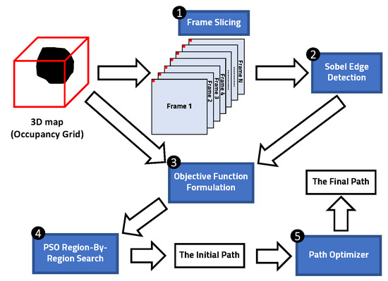
Figure 1.
A general block-diagram illustration of the proposed SPF path planning system.
It is worth noting that the proposed SPF technique is a global offline path planning technique. Therefore, it is not concerned with the process of building the occupancy grid and generating the 3D map of the environment. Similar to other offline path planning techniques including A*, D*, and other techniques, the process of the proposed SPF technique begins after building the map of the environment.
3.1. Frame Slicing
The input data is a 3D map formatted in a 3D occupancy grid. Occupancy grids represent a map of the environment as a set of binary random variables distributed spatially as equal-sized non-overlapping blocks representing the presence of an obstacle at the location in the environment. In a simpler form, an occupancy grid is pixel-oriented 3D data, where 0s’ represent obstacles, while the 1s’ represent the obstacle-free area in the 3D map or vice versa. The variables x, y, and z are the dimensions of the map where x and y denote the width and the height of the map, while z denotes the depth of the map. The first step of the proposed SPF path planning system is to slice the input 3D map into its composing frames , , , , , where: , , where N is the last frame which equals to the maximum value of z. For example, if the input map has a size of , then .
3.2. Sobel Edge Detection
The next step is to apply the Sobel edge detection technique on each frame separately. In digital images, an edge is a high-frequency component of an image since the gray-level intensity values witness a rapid abrupt change across an edge area. For a binary occupancy grid, where obstacle and obstacle-free areas are distinguished by two distinctive colors, an edge represents a critical aspect of the map as it locates the boundary of the obstacles on the map. In an occupancy grid, the edge of an obstacle is reflected in the discontinuity of the black pixels in a certain direction.
Sobel detector is an orthogonal gradient operator. Let be a continuous function, the gradient at is expressed as a vector:
The magnitude and angle of the gradient vector are:
Theoretically, the partial derivatives of Equation (1) should be calculated for every pixel in the image. However, for a discrete digital image, convolution is used instead. The input image is convolved with two small templates that inherit the properties of horizontal and vertical edges. The templates are scanned through the entire image, and when there is a match between the mask and the area under the mask, the convolution output will be maximized. The following are the masks utilized to find edges:
These masks are going to be convolved with the input image to find edge locations:
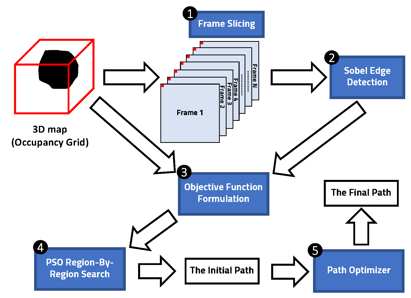
Finally, edge points are found in c by tracing high values. This can be done using a proper threshold value. Figure 2 shows the output of the sobel operator on a slice of a 3D map. More information about Sobel edge detection technique can be found in [31].
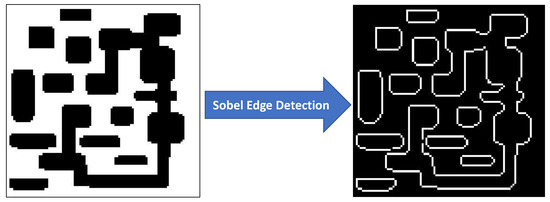
Figure 2.
The sobel edge detection algorithm is applied to a slice of the 3D map.
3.3. Objective Function Formulation
The goal of a path planning system is to obtain an obstacle-free path to the desired destination. The proposed SPF path planning system mimics the physical phenomenon of the electric potential field where some attractive and repulsive forces are present in the environment. The UAV should move away from obstacles and therefore, the proposed SPF technique suggests that obstacles should be the source of the repulsive forces on the map. On the other hand, the UAV should always be heading towards the goal point and therefore, the goal point should emit attractive forces on the map.
The attractive and repulsive forces must be modeled differently. To be able to reach the desired destination from any point on the map, the attractive force emitted from the goal point should be sensed everywhere on the map. Therefore, the attractive force emitted by the goal point will act as the UAV guider to the desired destination from any point on the map. On the other hand, the strength of the emitted repulsive forces from obstacles should be a function of the distance from the obstacle. The UAV should receive a very strong repulsive force from a certain obstacle when being very close to the obstacle, while the strength of the repulsive force should decay while moving away from the obstacle. That is since a far-away obstacle does not pose a threat to the UAV.
To efficiently model the effects of the repulsive and attractive forces in a 3D map, the proposed SPF path planning system develops an objective function over each pixel located at on the map. The objective function is designed so that the goal point will be the global minimum point on the map, while locations containing the edges of the obstacles will have high values. Therefore, by minimizing the objective function of over sequential non-overlapping areas, the UAV will be able to navigate to the desired destination without colliding with an obstacle.
The proposed SPF path planning system adopts the 3D Euclidean distance to model the attractive force emitted by the goal point. The Euclidean distance is chosen since the strength of the attractive force emitted by the goal point should be linearly related to the distance. The election of the Euclidean distance will enable the attractive force to be sensed strongly all over the 3D map. Therefore, the UAV will always have an active guider to the desired destination.
On the other hand, the strength of the repulsive forces generated by obstacles should be very strong around obstacles but should decay after some distance. Therefore, the proposed SPF path planning strategy models the repulsive forces similarly to Coulomb’s law. This is done by treating the UAV as a unit test charge in an electrical potential field caused by obstacles. Based on Coulomb’s law, the strength of the electric field is inversely proportional to the square of the distance from the charge causing the field. This fact makes it suitable to adopt Coulomb’s law to model the repulsive forces produced by obstacles.
The objective function can be generally formulated as:
where is the 3D Euclidean distance between the point and the desired destination, while represents the strength of the repulsive force emitted by the obstacle k at the location , n is the total number of obstacles. Finally, and are tuning parameters.
The 3D Euclidean distance is defined as:
where , , and are the x, y, and z coordinates of the desired destination point.
The repulsive force emitted by the obstacle k is defined as:
where m is the total number of edge points of the obstacle k, r is the 3D Euclidean distance from the point to the obstacle edge. The points , , and are the x, y, and z coordinates of the edge point of the obstacle k.
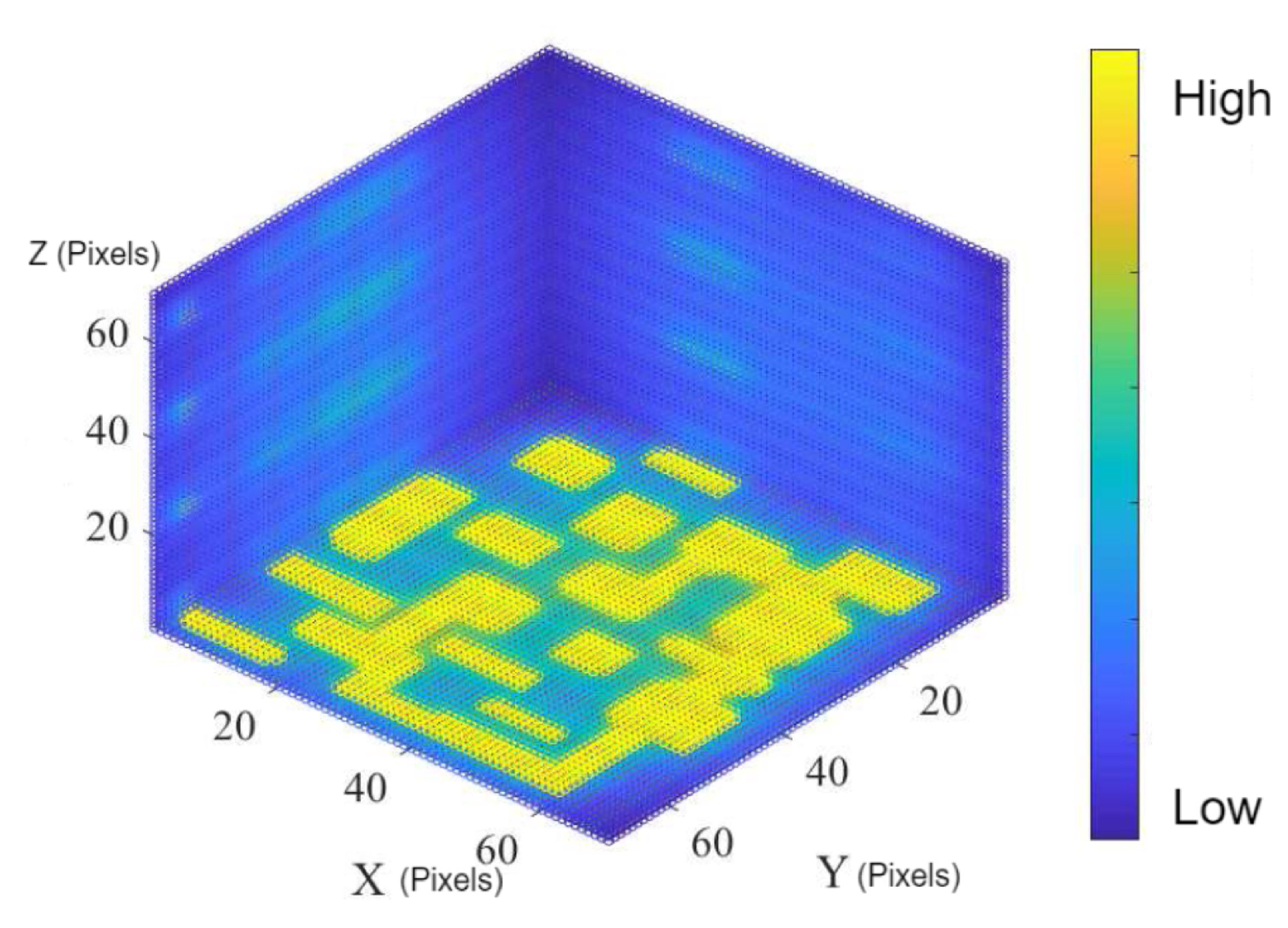
Figure 3 illustrates in a 3D plot, the implementation of the objective function derived in Equation (11).

Figure 3.
A slice of the 3D map shows the implementation of the objective function derived in Equation (11). The shown 3D map is built from the 2D map shown in Figure 2. The objective function was successful in developing strong repulsive forces in the areas containing the obstacles and the areas surrounding the obstacles.
3.4. The Initial Waypoint Generator: The PSO Region-by-Region Search
To obtain the waypoints, the Particle Swarm Optimization technique (PSO) is adopted to minimize the objective function derived in Equation (11). However, optimizing the objective function will return a single global minimum value which is the goal point. A feasible path is a set of sequential points. Therefore, the proposed SPF technique suggests performing several sequential searchers which start at the starting point and end at the goal point.
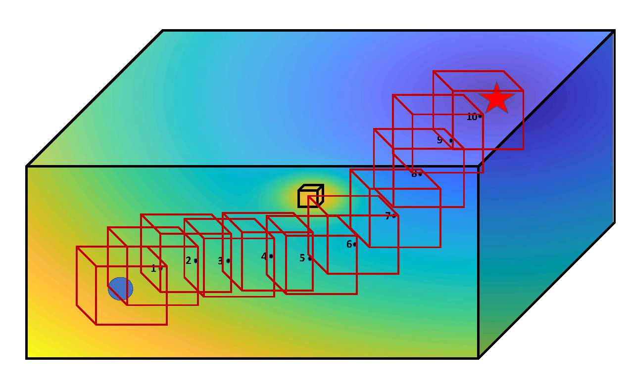
The PSO region-by-region search adopted by the proposed SPF scheme begins by performing a search for the minimum value around the starting point within a 3D area. Next, the new search area will be centralized around the newly founded optimum value. The search area keeps moving until the goal point is found to be located in the updated search area. Figure 4 shows an illustration of the procedure utilized to obtain the initial path.

Figure 4.
Illustrating The 3D region-by-region search algorithm used to generate the initial waypoints. The blue circle is the starting point and the red star is the goal point. The black dots are the optimum solutions founded by the PSO technique in each 3D search region. The black cube represents a 3D obstacle.
3.5. Path Optimizer
The path produced by the PSO sequential searches is not an optimal path. The path is optimized by using a shortening algorithm. The main objective of the shortening algorithm is to look for any possible obstacle-free linear shortcut between any two points in the path. The optimizing process is done in two phases. The first phase tries to find any possible shortcuts on the path obtained by the PSO search. The second phase tries to find the shortcuts on the path produced by the first phase. The output of the second phase is composed of sequential linear paths which can contain sharp turns. Such paths can cause difficulties for controllers. It is not a trivial task to track a path with sharp turns. Therefore, the quality of the path is further enhanced by smoothing the path using cubic interpolation. The path obtained by the second phase consists of discrete points. By interpolating these points using cubic interpolation, the path is guaranteed to be as smooth as enough to be easily tracked by the controller. The smoothed path will be adjacent to the obstacle-free path obtained by the second phase. However, there is a small probability that the smoothed path will pass through an obstacle area. In such a case, the smoothed path will be ignored and the final SPF path will be the output of the second phase.
4. Experimental Results
In this section, the performance of the proposed SPF path planning system will be examined against the swiftness-quality trade-off. Moreover, the trackability of the proposed path will be tested experimentally. Section 4.1 presents the setup used for the experiments. Section 4.2 conducts comprehensive experiments to evaluate the proposed SPF path planning system against the swiftness-quality trade-off. A discussion on the parameters of and and their role in solving potential field problems is presented in Section 4.3. Finally, Section 4.4 shows the experiments conducted to test the smoothness and the trackability degree of the proposed SPF path planning system. Figure 5 and Figure 6 show the Parrot quadcopter system and the experimental setup block diagram, respectively. Figure 7 and Figure 8 show visually the different maps that were used in the experiments. Figure 9 shows the final path generated by the proposed SPF path planning scheme on the different maps. The maps were developed manually by creating an empty 3D occupancy grid and then filling the positions of the obstacles in the grid that reflect the physical environment. The dimensions of the maps are shown in pixels for generalization purposes. In our experiments, each pixel corresponds to 0.01 m.
4.1. Experimental Setup
The experiments were performed in an indoor environment using the parrot mambo system shown in Figure 5. The specifications of the parrot mambo drone including the processing power and the available sensors are shown in Table 1.

Table 1.
The technical specifications of the Parrot Mambo drone.
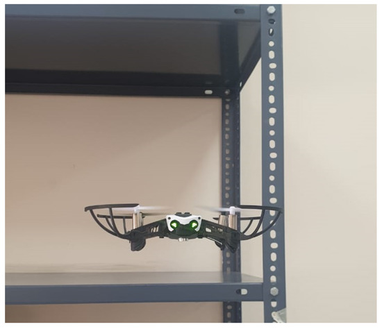
Figure 5.
The UAV system used in the experiment (Parrot Mambo).
Figure 5.
The UAV system used in the experiment (Parrot Mambo).

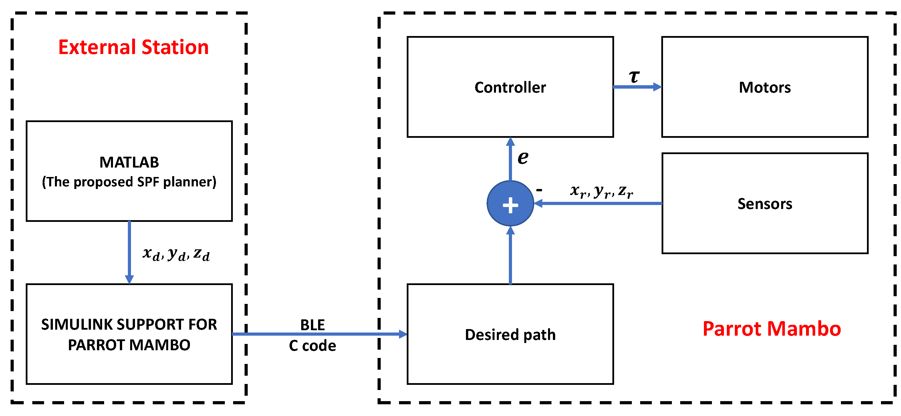
Figure 6 shows a block diagram which explains the setup used for the experiments. Based on Figure 6, the proposed SPF path planning technique is first executed on an external station with an Intel Xeon E3-1545M v5 processor at 2.90 GHz, and a RAM capacity of 32 GB. The external station is equipped with the Simulink Support Package for Mambo drone which contains the necessary tools to debug and deploy the code into the micro-controller of the drone wirelessly using Bluetooth Low Energy (BLE) technology. Figure 6 shows that the control code is based on a feedback control system. The controller receives an error signal e between the desired path calculated by the proposed SPF path planning technique and generates the required torque commands which will be sent to the motors in order to be able to track the desired path.
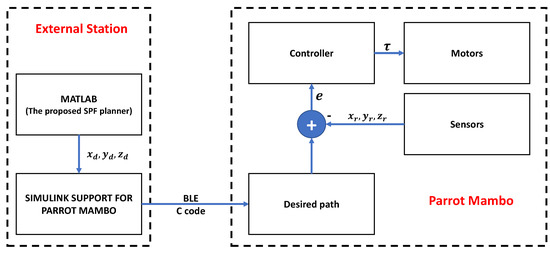
Figure 6.
The experimental setup.
Figure 6.
The experimental setup.
4.2. Swiftness-Quality Trade-Off Analysis
This subsection evaluates the behavior of the proposed SPF path planning technique against the swiftness-quality trade-off problem. Section 4.2.1 compares the proposed SPF technique with well-known path planning techniques such as 3D-A* and 3D-PRM techniques. The proposed SPF technique is compared with other potential field techniques in Section 4.2.2. Section 4.2.3 compares the proposed SPF which uses PRM as an optimization tool with another meta-heuristic optimization technique which is the Genetic Algorithm (GA). Finally, Section 4.2.4 examines the effect of the population parameter on the performance of the proposed SPF path planning technique.
4.2.1. Comparison against 3D-A* and 3D-PRM
Table 2 shows comparative results on the performance of the proposed SPF path planning technique against two well-known and widely used path planning techniques, the A* and the PRM techniques. The comparison examines the performance of the three techniques in terms of the path length and the execution time.
Table 2.
Comparing the performance of the proposed technique against two well-known path planning algorithms the 3D-A* [26] and 3D-PRM [20]. The block size column shows a percentage of the dimension of the search block with reference to the dimension of the map.
Table 2 clearly shows the superior performance of the proposed SPF path planning technique over well-known path planning algorithms such as A* and PRM in terms of the time required to obtain the obstacle-free path. It is clear from Table 2 that the large improvement in the swiftness attribute did not significantly affect the path length, which proves the ability of the proposed SPF technique to overcome the traditional trade-off between swiftness and path length. The proposed SPF has achieved high improvement percentages reaching up to 445.33% which corresponds to a record of “5.45×” faster execution. This record has been achieved when applying the proposed SPF technique in map 1 when having a search block dimension length of 15% of the dimension of the map. The interesting fact about this 445.33% improvement is that it was able to achieve equivalent path lengths to A* and PRM. According to Table 2, the proposed SPF path planning technique is executed in 0.75 s producing a path length of 1.73 m, while A* and PRM have executed in 2.87 s and 4.09 s producing paths of 1.71 m and 1.69 m respectively. The increase in the path length is less than 0.025% which is not comparable to the improvement in the processing time (445.33%).
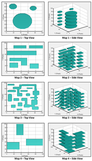
Figure 7.
Showing Map 1, Map 2, Map 3, and Map 4.
Figure 7.
Showing Map 1, Map 2, Map 3, and Map 4.
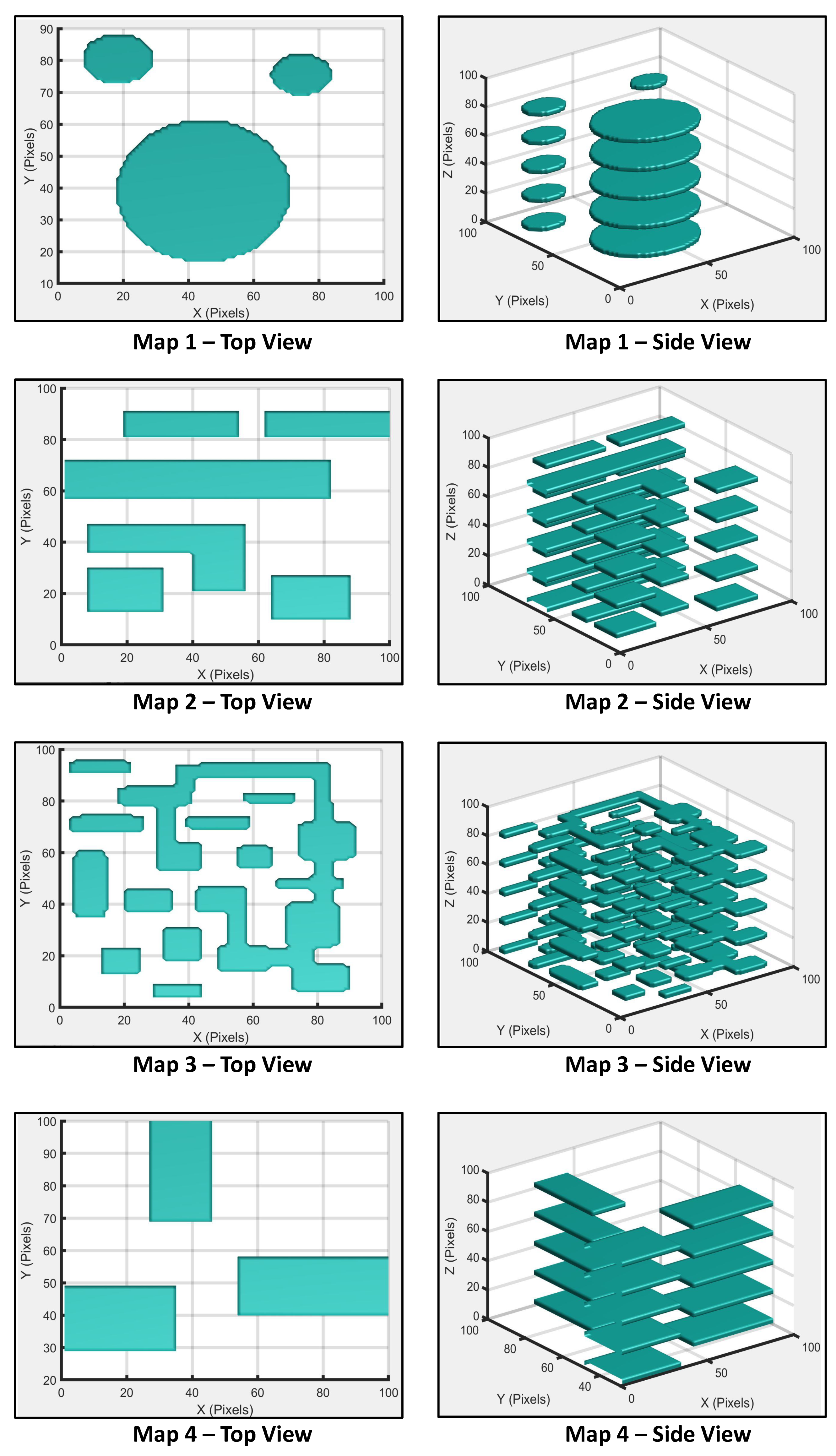

Figure 8.
Showing Map 5, Map 6, and Map 7.
Figure 8.
Showing Map 5, Map 6, and Map 7.
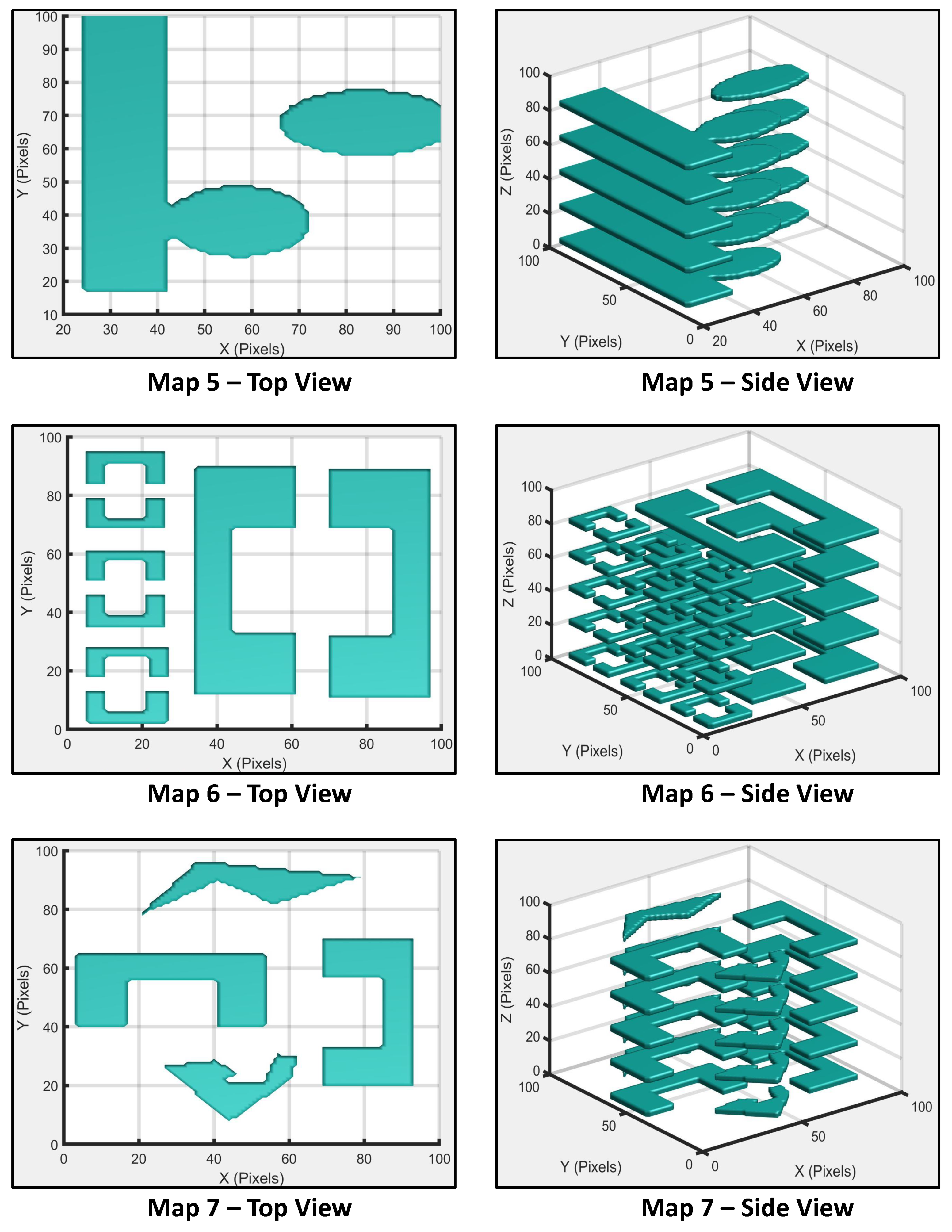
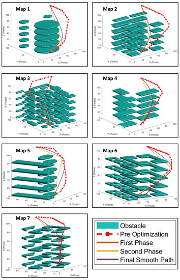
Figure 9.
The final path produced by the proposed SPF scheme on different 3D maps.
Figure 9.
The final path produced by the proposed SPF scheme on different 3D maps.
Another noticeable fact from Table 2 is that the proposed SPF technique was always able to achieve faster execution than A* and PRM for all maps. The interesting unexpected result is that even though the proposed SPF technique has outperformed the A* and PRM techniques in terms of the execution speed, the proposed SPF technique has also achieved shorter paths than the competitive techniques in some scenarios. For example, when testing with map 4, the proposed SPF technique has achieved a path length of 1.52 m compared to 1.60 m for A*. These results were achieved while having an improvement percentage in the processing time reached a rate of 5.40×.
The superior performance of the proposed SPF technique in terms of the computational speed can be attributed to the potential field idea and the PSO optimization technique. The processing required by a potential field algorithm is lower compared to the search process required by a graph-base technique such as the A*, or a sampling-based technique such as PRM. Simply put, the potential field algorithm only requires an objective function to be optimized on the map. Moreover, it is widely known that the PSO optimization technique is a fast-converging technique as will be proven in Section 4.2.3. Therefore, optimizing a fast-execution objective function using a fast optimization function will produce an overall fast path planning system as in the proposed SPF technique. On the other hand, the advancement in the quality of the path produced by the proposed SPF technique can be attributed to the optimization phases. The optimization phases find linear shortcuts in the path obtained by the PSO and thus, it is expected that the length of the final path of the proposed SPF technique will be acceptable.
The search block size is a critical parameter that affects the performance of the proposed SPF technique. From Table 2, the size of the search block has affected both, the computational time and the path lengths. Based on Table 2, decreasing the block size increases the computational time. The reason is that by using smaller block sizes, more searches are needed until the search block reaches the goal point. However, choosing a small block size can in some cases enhance the final path. The reason is that searching within smaller blocks is more accurate and the path can be obtained more precisely than larger blocks.
The experiments shown in Table 2 and Figure 9 have fixed starting point and goal point. These experiments have used extreme cases where the starting point is at one edge of the map, and the goal point is at the opposing edge. This means that the path will pass through the whole map which ensures the credibility of the results. However, it is also valuable to check the performance of the proposed SPF technique when using different starting points and goal points. Table 3 shows a comparative analysis between the proposed SPF technique and the techniques of 3D-A* and 3D-PRM using various starting points and goal points. Similar to the results obtained in Table 2, the results shown in Table 3 support the claims of the superior performance of the proposed SPF technique in terms of the execution speed. Even though the main concern of the proposed SPF technique is to obtain fast-executable pats, the results shown in Table 3 have even shown that the proposed SPF technique can obtain reduced path lengths compared to 3D-A* and 3d-PRM techniques.
Table 3.
Comparing the performance of the proposed technique against 3D-A* [26] and 3D-PRM [20] techniques when changing the start and goal points. Length is in meters while the execution time is computed in seconds.
4.2.2. Comparison with Potential Field Techniques
This section compares the performance of the proposed SPF technique against 1st-order and 2nd-order potential field techniques. Table 4 shows a comparison between the proposed SPF technique and the potential field methods. Although the proposed SPF technique can be considered as a potential field technique, the results in Table 4 have shown improved results over the 1st-order and 2nd-order potential field techniques. The general reason for these advanced results is that the proposed SPF technique is also equipped with other techniques that enhance the overall performance of the technique. For example, it is clear from Table 4 that the proposed SPF technique was able to achieve shorter path lengths compared to 1st-order and 2nd-order potential field techniques for all maps. The reduced path length produced by the proposed SPF technique compared to potential field methods is attributed to the path optimizer phase described in Section 3.5. For example, the proposed SPF technique was able to achieve a path length of 1.74 m compared to 2.75 m and 2.92 m achieved by the 1st-order and 2nd-order potential field techniques when using map 3.
Table 4.
Comparing the performance of the proposed SPF technique against 1st-order and 2nd-order potential field. The block size column shows a percentage of the dimension of the search block with reference to the dimension of the map.
Potential field techniques are known for their fast execution. Therefore, based on Table 4, the 1st-order and 2nd-order potential field techniques were able to generate the obstacle-free path in a short time. However, the proposed SPF technique was still able to execute in a shorter time compared to 1st-order and 2nd-order potential field techniques. For all maps, the path produced when planning with a block size of 15% is always computed faster than the 1st-order and the 2nd-order potential field techniques. For example, the proposed SPF technique was able to execute within 1.61 s compared to 3.96 s and 3.72 s for 1st-order and 2nd-order potential field techniques which makes the proposed SPF faster by rates of 2.46× and 2.31× respectively. The reason for the superior execution speed of the proposed SPF technique is attributed to two factors: adopting the PSO technique which is known for its fast execution. The second factor is attributed to the process of confining the emitting of the repulsive forces to be only from the edges of the obstacles. Therefore, the execution processes will be reduced compared to potential field techniques which result in faster execution speeds.
4.2.3. Comparison with GA
This subsection compares the proposed SPF path planning technique against the Genetic Algorithm optimization technique. The proposed SPF path planning technique adopts the PSO optimization strategy. The goal of this section is to prove the superior performance of the PSO technique over other meta-heuristic optimization techniques such as GA. Table 5 shows comparative results on the performance of the proposed SPF technique adopting PSO against adopting the GA algorithm in terms of the path length and the execution time.
Table 5.
Comparing the performance of the proposed SPF technique against the meta-heuristic technique the Genetic Algorithm. The block size column shows a percentage of the dimension of the search block with reference to the dimension of the map.
It is clear from Table 5 that the PSO algorithm can converge quicker and obtain the optimum obstacle-free path in a shorter time than GA. All cases have shown superior performance of the proposed PSO-based SPF technique compared to the GA technique. It is widely known in the literature that the PSO optimization algorithm has the ability to converge quicker than other heuristic optimization methods [30]. The reason is that the PSO algorithm has no crossover and mutation operations such as the GA method and thus, the convergence can occur by the particle speed. Only the best particle can exchange the information with other particles, which increases the convergence speed [30].
The path lengths of both the proposed SPF and the GA algorithms are almost identical based on the results of Table 5. However, in some cases, even though the proposed technique (PSO) was able to execute within a shorter period of time, the proposed PSO has achieved a shorter path than GA. This fact can conclude that the proposed PSO-based SPF algorithm was able to surpass another meta-heuristic optimization algorithm which is the GA algorithm and can successfully challenge the trade-off problem between path length and the swiftness attributes.
4.2.4. The Effect of the PSO Population
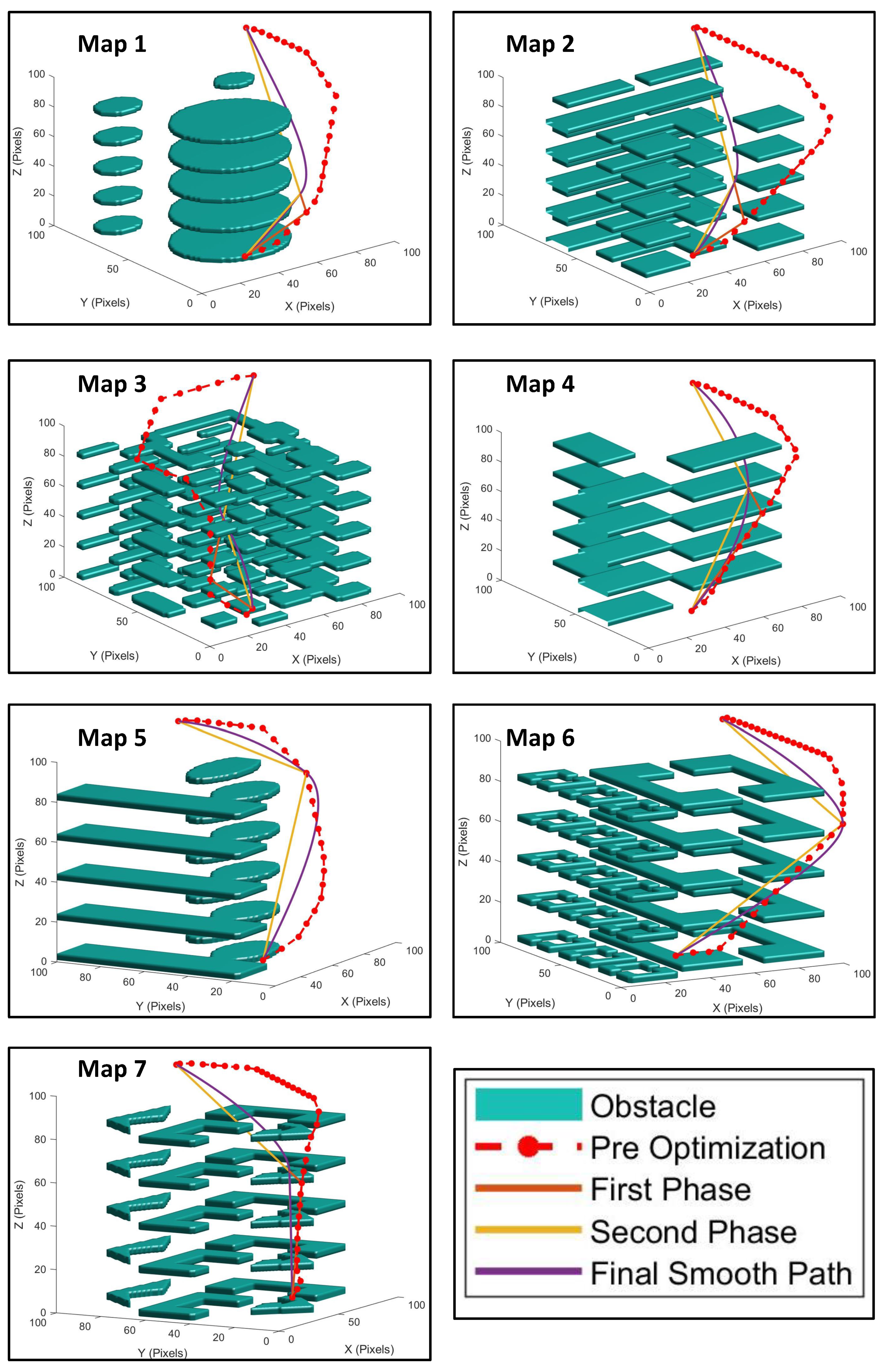
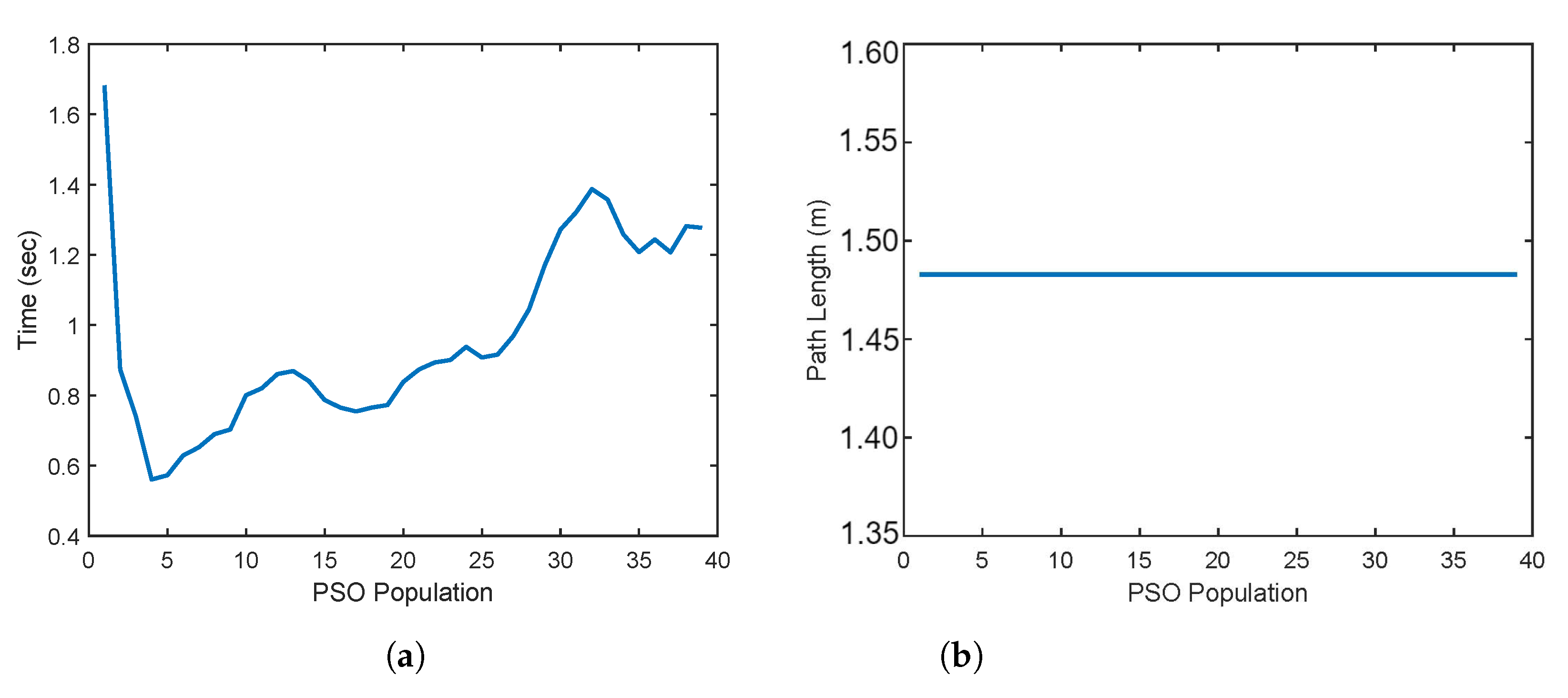
In this section, the effect of tuning the PSO population parameter on the computation speed and on the path length is investigated. Figure 10 presents a graph that represents the different results obtained when tuning the PSO population parameter. Figure 10a shows the effect on the computation speed, while Figure 10b shows the effect on the path length. Based on Figure 10a, a population size of around 5 gave the best result. Decreasing the population size to a value below 5 increases the computational time required to calculate the obstacle-free path. That is because searching for the optimum value with an insufficient number of particles (population) will naturally take more time than searching with a sufficient number of particles. However, increasing the population to higher than 15 gives an inverse effect, as the computational time increases. The reason for the time increase when choosing a high population value is that each extra particle requires additional processing and therefore, the computational time increases with the increase of the number of particles.
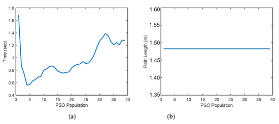
Figure 10.
The effect of tuning the PSO population parameter on the (a) processing speed, (b) path length.
On the other hand, Figure 10b clearly shows that tuning the PSO population parameter does not affect the path length. Based on Figure 10b, tuning the population parameter in the range [1–40] did not change the path length obtained by the proposed SPF technique. The reason is that regardless of the number of the particles, there is a strong probability that these particles will converge to the same optimum value, especially since the search area is not large (15% block size is the maximum). Within such a small area, having a small number of particles will affect the time needed to find the optimum value, not the optimal value itself.
4.3. Solving Potential Field Problems Using and Parameters
The purpose of the tuning parameters of and presented in Equation (8) is to control the strength of the attractive force and the repulsive forces. These parameters were added to the objective function for generalization purposes. By default, and are not used ( and ). However, the parameter can be thought of as a safety parameter. By increasing the value of , the repulsive force becomes stronger. Therefore, the robot will keep a safety distance from obstacles. However, increasing parameter to a very high value will make the repulsive force too stiff even that the robot will not be able to move due to the strong repulsive forces from all directions. Since the repulsive force is a function of distance from an obstacle, the acceptable range of depends on the size of the map. For the maps used in this paper, a value higher than 3 is not recommended and can cause the proposed SPF technique to fail.
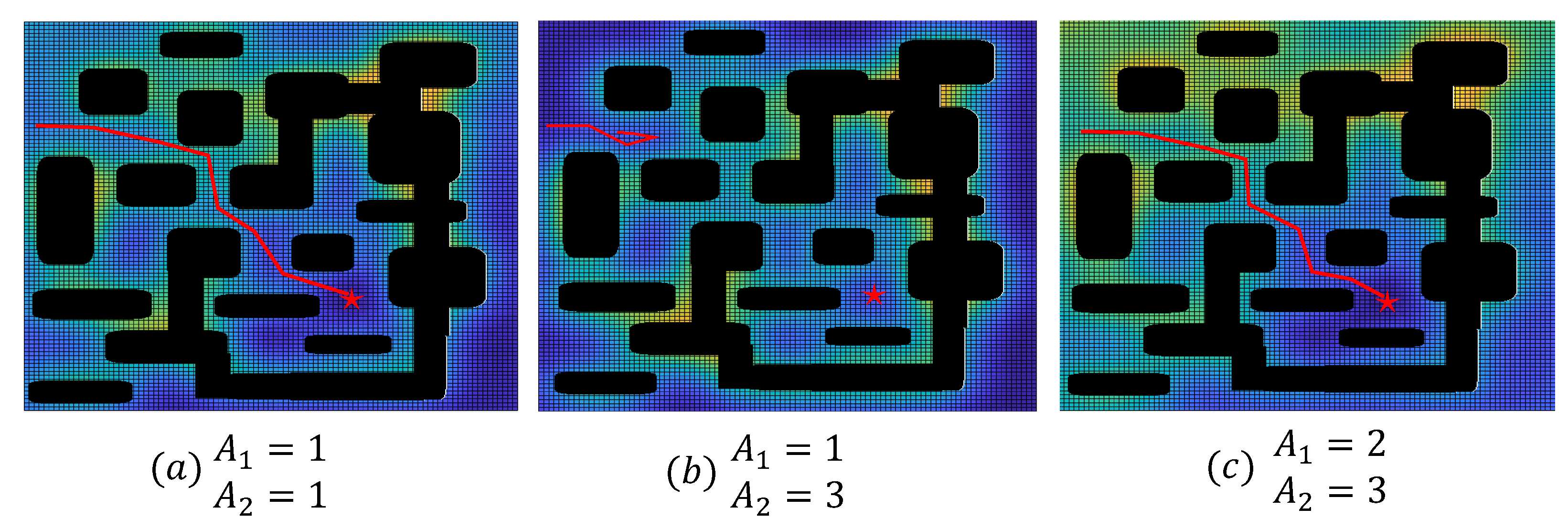
Figure 11 illustrates the effect of tuning the and parameters on the performance of the proposed SPF technique. For illustration purposes, the proposed SPF technique is implemented on a 2D map. It is clear from Figure 11a that even though the map contains areas that have the potential to cause a trap, the proposed planner is able to find a path to the goal point. The reason is attributed to the force modeling technique adopted by the proposed SPF technique. The repulsive forces are modeled using Coulomb’s law. Thus, the energy of the repulsive force will be very strong near the obstacle, but it will decay exponentially when moving away from the obstacle. This strong decay in the repulsive force will reduce the probability of causing a local trap even in a semi-closed area. Another well-known problem of a potential field path planning technique is the narrow passage problem. A potential field planner cannot plan a path through a narrow passage caused by two parallel obstacles due to the repulsive forces from the adjacent obstacles. However, based on Figure 11a, the proposed SPF planner is able to find the obstacle-free path even with several narrow passages. The reason for success here is attributed to the Euclidean force emitted by the goal point. Even if the goal point is located inside a semi-closed area where a narrow passage problem can occur, the attractive force from the goal will pull the robot through the narrow passage.
Figure 11.
The effect of tuning the and parameters. The star denotes the goal point.
However, the path generated in Figure 11a does not have a safety margin. The path passes nearby an obstacle. As explained earlier, a higher value of parameter can give a safety margin. However, the attempt to increase the parameter has failed as shown in Figure 11b. Increasing the parameter has caused a difference in the potential field values within the open areas compared to the narrow passage area. The narrow passage area now has a higher potential field value than the open area. Thus, the UAV will not be able to enter the narrow passage area. A solution to this problem is presented in Figure 11c. To force the planner to enter the narrow passage area, the Euclidean force (attractive force) from the goal point should be strengthened. This can be achieved by increasing the parameter as can be concluded from Equation (8). The Euclidean force is simply the distance from the goal point. By strengthening the Euclidean force, the areas that are far away from the goal point will have high potential field values. Based on Figure 11c, the open area next to the starting point has now a higher potential field value compared to the narrow passage area. Thus, the planner is “pushed” to enter the narrow passage area, and therefore, the proposed planner is able to obtain the path through the narrow passage area.
4.4. The Tracking Performance: Smoothness Test
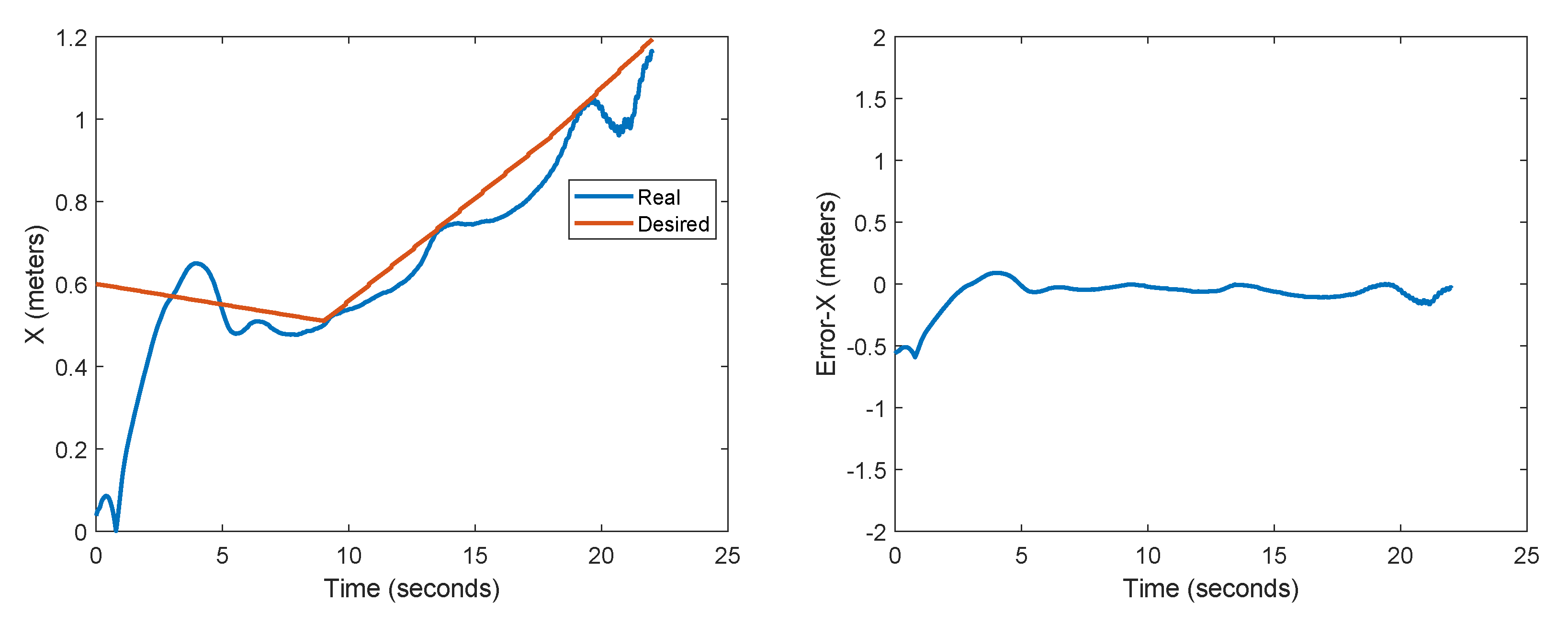
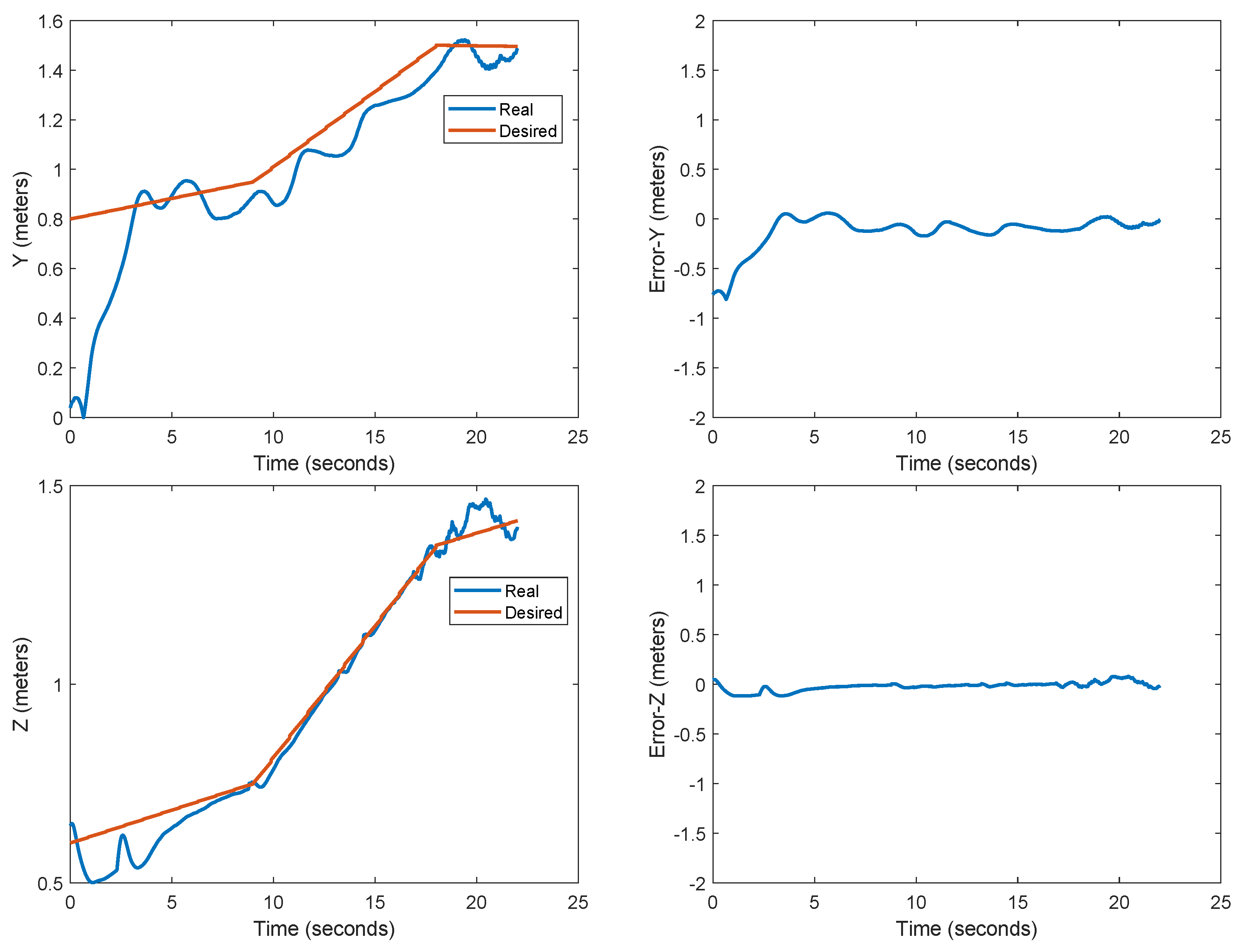
Finally, the trackability of the paths generated by the proposed SPF path planning algorithm is tested using a basic Proportional-Integral-Derivative (PID) controller. The goal of this experiment is to prove that the proposed SPF technique can produce paths which are smooth enough to be traced with good accuracy even when using simple PID controller.
Figure 12 illustrates the tracking performance of the proposed SPF path planning technique. It is clear from Figure 12 that the path produced by the proposed scheme is traceable with good tracking performance. The tracking errors in the x, y, and z planes approach zero. The reason for the smoothness of the paths produced by the proposed SPF technique is attributed to the optimization phases. The output of the second optimization phase is simply a path consisting of a few sequential linear paths, which can be controlled easily by any basic controller.
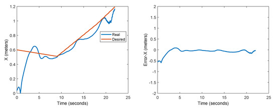
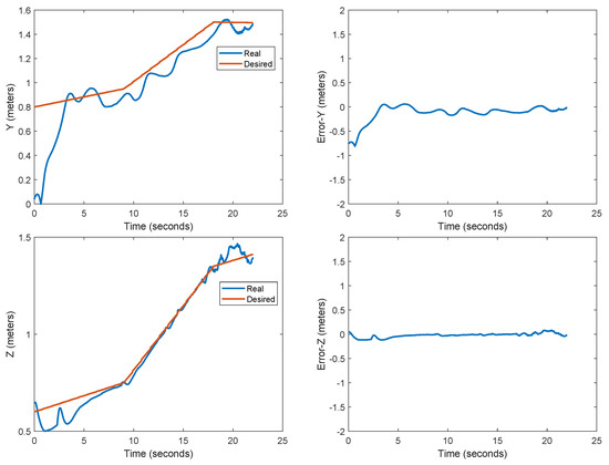
Figure 12.
The tracking performance of the proposed path planning scheme.
5. Conclusions
A new responsive path planning technique named Sobel Potential Field (SPF) was proposed for UAV systems. The objective of the proposed SPF technique was to effectively deal with the swiftness-quality trade-off problem of path planning algorithms. The main idea was to reduce the processing required by potential field techniques by focusing on obstacle areas instead of the whole 3D map. This is done by developing a 3D potential field caused by the edges of the obstacles detected by the Sobel edge detection algorithm. The attractive force will be generated by the goal point affecting each point on the map, while the edges of obstacles will be the source of repulsive forces affecting areas around obstacles. This has led to derive an objective function composed of a Euclidean distance and Coulomb’s law. The objective function is then optimized using PSO and a proposed optimization algorithm to find the best obstacle-free path to the destination. Experimental results concluded that the proposed SPF path planning algorithm can obtain the obstacle-free path quicker than other meta-heuristic optimization methods such as the GA algorithm, and even over popular path planning techniques such as A* and PRM, while producing a path with an equivalent or shorter length. Future work will focus on adapting the proposed SPF technique to operate with robotic manipulators and to deal effectively with the effects of the kinematics coupling of manipulators.
Author Contributions
Conceptualization, R.F.; Methodology, R.F. and M.B. (Mohammed Baziyad); Software, M.B. (Mohammed Baziyad); Validation, M.B. (Mohammed Baziyad) and R.F.; Formal Analysis, R.F. and T.R.; Investigation, M.B. (Mohammed Baziyad); Resources, M.B. (Mohammed Baziyad) and T.R.; Writing—Original Draft Preparation, R.F. and M.B. (Mohammed Baziyad); Writing—Review & Editing, M.B. (Mohammed Baziyad), R.F., T.R., I.K. and M.B. (Maamar Bettayeb); Visualization, M.B. (Mohammed Baziyad); Supervision, T.R., I.K. and M.B. (Maamar Bettayeb). All authors have read and agreed to the published version of the manuscript.
Funding
This research received no external funding.
Institutional Review Board Statement
Not applicable.
Informed Consent Statement
Not applicable.
Conflicts of Interest
The authors declare no conflict of interest.
References
- Chatziparaschis, D.; Lagoudakis, M.G.; Partsinevelos, P. Aerial and ground robot collaboration for autonomous mapping in search and rescue missions. Drones 2020, 4, 79. [Google Scholar] [CrossRef]
- Wahab, I.; Hall, O.; Jirström, M. Remote sensing of yields: Application of uav imagery-derived ndvi for estimating maize vigor and yields in complex farming systems in sub-saharan africa. Drones 2018, 2, 28. [Google Scholar] [CrossRef] [Green Version]
- Arroyo-Mora, J.P.; Kalacska, M.; Inamdar, D.; Soffer, R.; Lucanus, O.; Gorman, J.; Naprstek, T.; Schaaf, E.S.; Ifimov, G.; Elmer, K.; et al. Implementation of a UAV–hyperspectral pushbroom imager for ecological monitoring. Drones 2019, 3, 12. [Google Scholar] [CrossRef] [Green Version]
- Zefri, Y.; ElKettani, A.; Sebari, I.; Ait Lamallam, S. Thermal infrared and visual inspection of photovoltaic installations by UAV photogrammetry—Application case: Morocco. Drones 2018, 2, 41. [Google Scholar] [CrossRef] [Green Version]
- Larrinaga, A.R.; Brotons, L. Greenness indices from a low-cost UAV imagery as tools for monitoring post-fire forest recovery. Drones 2019, 3, 6. [Google Scholar] [CrossRef] [Green Version]
- Li, X.; Tan, J.; Liu, A.; Vijayakumar, P.; Kumar, N.; Alazab, M. A novel UAV-enabled data collection scheme for intelligent transportation system through UAV speed control. IEEE Trans. Intell. Transp. Syst. 2020, 22, 2100–2110. [Google Scholar] [CrossRef]
- Chen, D.; Qi, Q.; Zhuang, Z.; Wang, J.; Liao, J.; Han, Z. Mean field deep reinforcement learning for fair and efficient UAV control. IEEE Internet Things J. 2020, 8, 813–828. [Google Scholar] [CrossRef]
- Yang, K.; Yang, G.Y.; Fu, S.I.H. Research of control system for plant protection UAV based on Pixhawk. Procedia Comput. Sci. 2020, 166, 371–375. [Google Scholar] [CrossRef]
- Hulett, D.T. Schedule risk analysis simplified. PM Netw. 1996, 10, 23–30. [Google Scholar]
- Zhang, Y.; Chen, J.; Shen, L. Real-time trajectory planning for UCAV air-to-surface attack using inverse dynamics optimization method and receding horizon control. Chin. J. Aeronaut. 2013, 26, 1038–1056. [Google Scholar] [CrossRef] [Green Version]
- Madkour, A.; Aref, W.G.; Rehman, F.U.; Rahman, M.A.; Basalamah, S. A survey of shortest-path algorithms. arXiv 2017, arXiv:1705.02044. [Google Scholar]
- Polychronopoulos, G.H.; Tsitsiklis, J.N. Stochastic shortest path problems with recourse. Netw. Int. J. 1996, 27, 133–143. [Google Scholar] [CrossRef]
- Baziyad, M.; Nassif, A.B.; Rabie, T.; Fareh, R. Comparative Study on the Performance of Heuristic Optimization Techniques in Robotic Path Planning. In Proceedings of the 2019 3rd International Conference on Advances in Artificial Intelligence, Istanbul, Turkey, 26–28 October 2019; pp. 157–161. [Google Scholar]
- Fareh, R.; Rabie, T.; Grami, S.; Baziyad, M. A vision-based kinematic tracking control system using enhanced-prm for differential wheeled mobile robot. Int. J. Robot. Autom. 2019, 34, 206–221. [Google Scholar] [CrossRef]
- Fareh, R.; Baziyad, M.; Rahman, M.H.; Rabie, T.; Bettayeb, M. Investigating reduced path planning strategy for differential wheeled mobile robot. Robotica 2020, 38, 235–255. [Google Scholar] [CrossRef]
- Fareh, R.; Baziyad, M.; Rabie, T.; Bettayeb, M. Enhancing path quality of real-time path planning algorithms for mobile robots: A sequential linear paths approach. IEEE Access 2020, 8, 167090–167104. [Google Scholar] [CrossRef]
- Sun, Y.; Ran, X.; Zhang, G.; Xu, H.; Wang, X. AUV 3D path planning based on the improved hierarchical deep Q network. J. Mar. Sci. Eng. 2020, 8, 145. [Google Scholar] [CrossRef] [Green Version]
- Huang, Y.; Chen, J.; Wang, H.; Su, G. A method of 3D path planning for solar-powered UAV with fixed target and solar tracking. Aerosp. Sci. Technol. 2019, 92, 831–838. [Google Scholar] [CrossRef]
- Hwang, Y.K.; Ahuja, N. A potential field approach to path planning. IEEE Trans. Robot. Autom. 1992, 8, 23–32. [Google Scholar] [CrossRef] [Green Version]
- Kavraki, L.E.; Svestka, P.; Latombe, J.C.; Overmars, M.H. Probabilistic roadmaps for path planning in high-dimensional configuration spaces. IEEE Trans. Robot. Autom. 1996, 12, 566–580. [Google Scholar] [CrossRef] [Green Version]
- LaValle, S.M. Rapidly-Exploring Random Trees: A New Tool for Path Planning. 1998. Available online: http://msl.cs.illinois.edu/~lavalle/papers/Lav98c.pdf (accessed on 24 June 2022).
- Yang, L.; Qi, J.; Song, D.; Xiao, J.; Han, J.; Xia, Y. Survey of robot 3D path planning algorithms. J. Control Sci. Eng. 2016, 2016, 7426913. [Google Scholar] [CrossRef] [Green Version]
- Mohammed, H.; Romdhane, L.; Jaradat, M.A. RRT* N: An efficient approach to path planning in 3D for Static and Dynamic Environments. Adv. Robot. 2021, 35, 168–180. [Google Scholar] [CrossRef]
- Bailey, J.P.; Nash, A.; Tovey, C.A.; Koenig, S. Path-length analysis for grid-based path planning. Artif. Intell. 2021, 301, 103560. [Google Scholar] [CrossRef]
- Panov, A.I.; Yakovlev, K.S.; Suvorov, R. Grid path planning with deep reinforcement learning: Preliminary results. Procedia Comput. Sci. 2018, 123, 347–353. [Google Scholar] [CrossRef]
- Hart, P.E.; Nilsson, N.J.; Raphael, B. A formal basis for the heuristic determination of minimum cost paths. IEEE Trans. Syst. Sci. Cybern. 1968, 4, 100–107. [Google Scholar] [CrossRef]
- Stentz, A. Optimal and efficient path planning for partially known environments. In Intelligent Unmanned Ground Vehicles; Springer: Berlin/Heidelberg, Germany, 1997; pp. 203–220. [Google Scholar]
- Przybylski, M.; Putz, B. D* Extra Lite: A Dynamic A* with search-tree cutting and frontier-gap repairing. Int. J. Appl. Math. Comput. Sci. 2017, 27, 273–290. [Google Scholar] [CrossRef] [Green Version]
- Kovács, B.; Szayer, G.; Tajti, F.; Burdelis, M.; Korondi, P. A novel potential field method for path planning of mobile robots by adapting animal motion attributes. Robot. Auton. Syst. 2016, 82, 24–34. [Google Scholar] [CrossRef]
- Baziyad, M.; Saad, M.; Fareh, R.; Rabie, T.; Kamel, I. Addressing Real-Time Demands for Robotic Path Planning Systems: A Routing Protocol Approach. IEEE Access 2021, 9, 38132–38143. [Google Scholar] [CrossRef]
- Nausheen, N.; Seal, A.; Khanna, P.; Halder, S. A FPGA based implementation of Sobel edge detection. Microprocess. Microsyst. 2018, 56, 84–91. [Google Scholar] [CrossRef]
Publisher’s Note: MDPI stays neutral with regard to jurisdictional claims in published maps and institutional affiliations. |
© 2022 by the authors. Licensee MDPI, Basel, Switzerland. This article is an open access article distributed under the terms and conditions of the Creative Commons Attribution (CC BY) license (https://creativecommons.org/licenses/by/4.0/).