Active Disturbance Rejection Control for the Robust Flight of a Passively Tilted Hexarotor

Abstract

This paper presents a robust control strategy for controlling the flight of an unmanned aerial vehicle (UAV) with a passively (fixed) tilted hexarotor. The proposed controller is based on a robust extended-state observer to estimate and reject internal dynamics and external disturbances at runtime. Both the stability and convergence of the observer are proved using Lyapunov-based perturbation theory and an ultimate bound approach. Such a controller is implemented within a highly realistic simulation environment that includes physics motors, showing an almost identical behavior to that of a real UAV. The controller was tested for flying under normal conditions and in the presence of different types of disturbances, showing successful results. Furthermore, the proposed control system was compared with another robust control approach, and it presented a better performance regarding the attenuation of the error signals.

1. Introduction

The increasing use of multirotor unmanned aerial vehicles (UAV) in a broad set of applications demands, in some cases, the use of six-degree-of-freedom (DOF) motions. In other words, simultaneous translational and rotational motions are required. For the case of quadrotors, six-DOF actuation is not possible, since they have only four actuators placed in a flat (co-planar) configuration. Increasing the number of rotors in such a flat configuration does not change the situation, even though they can cope with some actuation faults. Adding a tilting angle to the rotors produces forces so that the drone becomes a fully actuated device within the six-DOF Cartesian space. Such a tilting angle can be either fixed (passive) or actuated by an auxiliary motor (active).

In addition to external disturbances, such as vortexes, wind gusts, or payloads that might affect a UAV, another significant drawback often present when controlling real devices is the uncertainty about the parameters of the system’s dynamic model. Thus, a control problem for passively tilted hexarotors is that of flying to the target pose or trajectory with respect to the world reference frame and remaining steadily within some desired tolerances about them despite the external disturbances and inaccuracy of the dynamic model. In this context, control researchers and engineers have developed robust techniques in order to deal with dynamic systems’ disturbances and uncertainties, and the UAVs’ case is not an exception.

Several robust controllers for both tilted and non-tilted hexarotors can be found in the literature. In addition to PID-type controllers for non-tilted hexacopters [1,2], another common control technique for flat hexarotors is the active disturbance rejection control (ADRC)-type approach. The advantage of using these last controllers is that they can deal with external disturbances and do not depend on an accurate dynamic model. There are plenty of recently reported and successful regulation and tracking simulations using this control approach—or variations thereof—which is applied to both non-tilted and actively tilted hexarotors [3,4,5,6,7]; nevertheless, the closed-loop stability was only proved in [3,4], and the observer’s convergence proof was only present in [3]. It is worth remarking that in [3,4], the ADRC stability proof relied on the a priori. assumption that the total disturbance was bounded, which is not applicable to fully actuated multirotor UAVs, as is later explained in the text.

On the other hand, an extensive literature with successful simulations is also available for the robust control of passively tilted hexarotors. The robust integral of the sign of the error (RISE) [8], integral sliding-mode control (SMC) [9], adaptive SMC [10], and super twisting observer SMC [11] techniques have also been reported. It is worth mentioning that these control schemes are enhanced versions of the SMC to reduce its intrinsic chattering effect. Furthermore, an adaptive control scheme was also presented in a simulation [12]. Although this last technique is robust to parametric uncertainties, it is still susceptible to external disturbances. To the best of the authors’ knowledge, the only robust controllers reported in the literature that were implemented in actual passively tilted hexacopters are port-Hamiltonian-based approaches [13,14]; these passivity-based techniques suffer from time-varying parametric uncertainties and non-smooth disturbances.

In the context of the disturbance compensation of multirotor UAVs, the following problems have been found so far. (i) The use of a tilting angle for the rotors helps to produce six-DOF Cartesian motion; however, a significant drawback of actively tilting the rotors, despite the hardware implications, is that the actuator dynamics delay the instantaneous disturbance rejection [15]. (ii) ADRC-type techniques are robust estimation and compensation tools for external disturbances. Their main drawback is that the theory assumes that there exist bounds for the total disturbances, which are compounded by external wrenches and internal terms of the plant that are different from a representation of a cascade of integrators [16]. Such an assumption does not hold for the case of fully actuated multirotors, since state-dependent disturbances present in the model cannot be assumed to be bounded. In the literature, some other control approaches that rely neither on model accuracy nor on disturbance boundaries can be found, such as the artificial delay-based or adaptive sliding-mode approaches [17,18]. Even though such controllers are potentially applicable to tilted hexarotors, since they have already been tested on flat quadrotors, it has been found that ADRC has fewer tuning parameters than artificial delay-based control, and, at least for this application, ADRC does not suffer from the chattering effect.

This work addresses the robust flight problem of a passively tilted hexarotor. In order to deal with external disturbances and uncertainties, a robust control approach is implemented. Such a proposal falls within the ADRC category, since it rejects the disturbances by estimating and compensating for them using the proposed sliding-mode extended-state observer (SMESO). In addition, the observer’s stability and convergence are proved using Lyapunov-based perturbation theory and an ultimate bound approach. The developed controller is implemented on a custom hexarotor model (this model is available in the following repository: https://github.com/jocacace/Firmware (accessed on 4 August 2022)), which has been adequately adapted to have tilted rotors and to run within Gazebo (http://gazebosim.org (accessed on 4 August 2022)), a 3D simulator with physics motors that is almost identical to the real version of such a UAV. Both the controller and the robust ESO were executed as nodes of the Robotics Operating System (ROS) middleware (http://www.ros.org (accessed on 4 August 2022)), which allows the simultaneous execution of such algorithms. The experiments for testing the developed controller consisted of (i) performing a given trajectory, (ii) feeding target poses to the UAV such that it would fly under wind conditions and a payload provided by the simulator, and (iii) carrying out a comparison against an SMC for pose regulation. The contributions of this work are listed below.

• To the best of the authors’ knowledge, the application of the ADRC to a passively tilted hexarotor has not been reported. The closest related works use actively tilted or fixed hexarotors, which are disadvantaged in their actuation and disturbance rejection capabilities with respect to passively tilted hexarotors. Furthermore, our version of the ADRC technique is enhanced with a sliding-mode observer, whose advantages are mentioned later in the text.
• Both controller and observer stability analyses are presented. The implementation of an SMESO-based ADRC algorithm in a passively tilted hexarotor is novel in the literature to the best of the authors’ knowledge; furthermore, the stability proof of the presented ADRC does not depend on a priori assumptions of the boundaries of the total disturbance as the traditional ADRC scheme requests, but only on its differentiation properties.
• Our controller is implemented in a highly realistic simulation environment, which is completely different from a traditional numerical simulation. This is a step towards successful implementation on a real device, since our simulation scheme is almost identical with the real version of the platform. Additionally, our results are shown in a video.
• The comparison with another robust control and observation strategy favors the controller developed in this work. The proposed design is indeed a competitive alternative for the control of UAVs with passively tilted hexarotors, and it is not limited to the specific problem that is presented. The proposed controller applies to other passively tilted multirotors by selecting the appropriate allocation matrix, tuning both the controller and observer gains, and adjusting the integration steps.

The rest of this paper is organized as follows. Section 2 addresses the theory of ADRC, sliding-mode observers, and finding bounds for state-dependent disturbances; the dynamics of the hexarotor UAV are also presented in that section. Section 3 details the controller design and stability. Section 4 describes how the controller is implemented. Case studies are presented in Section 5, and finally, Section 6 concludes the paper.

2. Theoretical Background

ADRC is a control technique in which success relies on estimating and rejecting an unknown total disturbance using an ESO. In this case, a nonlinear control problem is reduced to a problem of a cascade of integrators. Therefore, this control technique can deal with a vast range of uncertainties and disturbances [16]. Below, an overview of the mentioned control approach and a robust observation scheme can be found. As stated before, the theory of ADRC relies on a priori assumptions of the existence of boundaries for the disturbances affecting the controlled system. For the case of external disturbances, such assumptions are reasonable; however, state-dependent disturbances cannot be assumed to be bounded. Hence, some useful theorems that were retrieved from the literature and are beneficial for the derivation of the stability proofs are also addressed in this section.

2.1. Active Disturbance Rejection Control

Consider the following multiple-input–multiple-output (MIMO) uncertain nonlinear system subjected to external disturbances [19], which is expressed in the canonical form of a chain of integrators (if the system is not represented in the canonical form of a chain of integrators, the corresponding transformations must be performed to lead the system to such a form).

$$\left\{\begin{array}{c}{\dot{x}}_{i,1}(t)=x_{i,2}(t)\hfill \\ {\dot{x}}_{i,2}(t)=x_{i,3}(t)\hfill \\ ⋮\hfill \\ {\dot{x}}_{i,n_i}(t)={\mathsf{\varsigma }}_i(\mathbf{x}(t))+{\mathsf{\xi }}_i(\mathbf{x}(t))\mathbf{u}(t)+{\mathsf{\zeta }}_i(t)\hfill \\ y_i(t)=h_i(\mathbf{x}(t))\hfill \end{array}\right.$$

(1)

with $i=1,\dots ,m$, and where $x_{i,j}(t)\in \mathbb{R}$ is a component of the vector state $\mathbf{x}(t)={\left[\begin{array}{ccccccc}{x}_{1,1}(t)& \cdots & x_{1,n_1}(t)& \cdots & x_{m,1}(t)& \cdots & x_{m,n_m}(t)\end{array}\right]}^T\in {\mathbb{R}}^{(n_1+\cdots +n_m)}$, with $j=1,\dots ,n_i$ and $n_i>0$; $y_i(t)\in \mathbb{R}$ is the $i-$th output component; $\mathbf{u}(t)=\left[\begin{array}{ccc}{u}_1(t)& \cdots & u_m(t)\end{array}\right]\in {\mathbb{R}}^m$ is the control input vector; $\mathsf{\varsigma }(\mathbf{x}(t))={\left[\begin{array}{ccc}{\varsigma }_1(\mathbf{x}(t))& \cdots & {\varsigma }_m(\mathbf{x}(t))\end{array}\right]}^T\in {\mathbb{R}}^m$ is the dynamic function with uncertain parameters; ${\mathsf{\xi }}_i(\mathbf{x}(t))\in {\mathbb{R}}^{1\times m}$ is the row of a non-singular uncertain matrix $\Xi \in {\mathbb{R}}^{m\times m}$ depending on the system’s state; $h_i(\mathbf{x}(t))\in \mathbb{R}$ is a function of the states; and $\mathsf{\zeta }(t)={\left[\begin{array}{ccc}{\zeta }_1(t)& \cdots & {\zeta }_m(t)\end{array}\right]}^T\in {\mathbb{R}}^m$ is the external disturbance vector, which is usually unknown but bounded. In order to reduce (1) to a regulation problem of a chain of integrators, the all of the uncertain dynamics and the external disturbances can be embedded into the following total disturbance [16]:

$$\mathsf{\varsigma }(\mathbf{x}(t))+{\Delta }_{\Xi }(\mathbf{x}(t))\mathbf{u}(t)+\mathsf{\zeta }(t)\triangleq \mathbf{x}{(t)}_{n+1},$$

(2)

where ${\Delta }_{\Xi }(\mathbf{x}(t))=\Xi (\mathbf{x}(t))-\tilde{\Xi }(\mathbf{x}(t))$ and $\tilde{\Xi }(\mathbf{x}(t))\in {\mathbb{R}}^{m\times m}$ is an approximation (in the context of this paper, the UAV’s approximated total mass and geometry can be useful in determining the numerical values of $\tilde{\Xi }(\mathbf{x}(t))$) of $\Xi (\mathbf{x}(t))$. The vector $\mathbf{x}{(t)}_{n+1}=\left[\begin{array}{c}{x}_{1,n_1+1}\cdots x_{m,n_m+1}\end{array}\right]\in {\mathbb{R}}^m$ is a virtual augmented state whose estimate $\widehat{\mathbf{x}}{(t)}_{n+1}\in {\mathbb{R}}^m$ contains all of the total disturbances, and it can be retrieved through the following ESO [19]:

$$\left\{\begin{array}{c}{\dot{\widehat{x}}}_{i,1}={\widehat{x}}_{i,2}+{\epsilon }^{n_i-1}{\varphi }_{i,1}\left({\displaystyle \frac{x_{i,1}-{\widehat{x}}_{i,1}}{{\epsilon }^{n_i}}}\right)\hfill \\ {\dot{\widehat{x}}}_{i,2}={\widehat{x}}_{i,3}+{\epsilon }^{n_i-2}{\varphi }_{i,2}\left({\displaystyle \frac{x_{i,1}-{\widehat{x}}_{i,1}}{{\epsilon }^{n_i}}}\right)\hfill \\ ⋮\hfill \\ {\dot{\widehat{x}}}_{i,n_i}={\widehat{x}}_{i,n_i+1}+{\varphi }_{i,n_i}\left({\displaystyle \frac{x_{i,1}-{\widehat{x}}_{i,1}}{{\epsilon }^{n_i}}}\right)+\tilde{\Xi }(\mathbf{x}(t))\mathbf{u}(t)\hfill \\ {\dot{\widehat{x}}}_{i,n_i+1}={\displaystyle \frac{1}{\epsilon }}{\Phi }_{i,n_i+1}\left({\displaystyle \frac{x_{i,1}-{\widehat{x}}_{i,1}}{{\epsilon }^{n_i}}}\right)\hfill \end{array}\right.$$

(3)

where ${\widehat{x}}_{i,j}(t)\in \mathbb{R}$ is a component of the vector state estimate

$$\widehat{\mathbf{x}}(t)={\left[\begin{array}{ccccccc}{\widehat{x}}_{1,1}(t)& \cdots & {\widehat{x}}_{1,n_1}(t)& \cdots & {\widehat{x}}_{m,1}(t)& \cdots & {\widehat{x}}_{m,n_m+1}(t)\end{array}\right]}^T\in {\mathbb{R}}^{(n_1+\cdots +(n_m+1))},$$

with $j=1,\dots ,n_i$ and $i=1,\dots ,m$; $\epsilon >0$ is a tuning constant, and ${\varphi }_{i,j}(·)\in \mathbb{R}$, with $j=1,\dots ,n_i+1$, is a function that guarantees $x_{i,1}-{\widehat{x}}_{i,1}\to 0$ as $t\to t_0,$ where $0<t_0<\infty$ is a determined finite time. Notice that the dynamics of (3) must be significantly quicker than those of (1). Once the total disturbance is estimated, it can be used as feedback in the following controller for the system (1):

$$\mathbf{u}(t)=\tilde{\Xi }{(\mathbf{x}(t))}^{-1}{\mathbf{u}}_0(\mathbf{x}(t))-\widehat{\mathbf{x}}{(t)}_{n+1},$$

(4)

where ${\mathbf{u}}_0(\mathbf{x}(t))\in {\mathbb{R}}^m$ can be any linear control technique that regulates $\dot{\mathbf{x}}(t)$. Since (4) cancels out both internal uncertainties and external disturbances, it leads to the following control problem:

$$\dot{\mathbf{x}}(t)\simeq {\mathbf{u}}_0(\mathbf{x}(t)).$$

(5)

2.2. Sliding-Mode Observers

As mentioned before, the success of the controller (4) relies on the accurate estimation of the total disturbance (2) via the ESO. Hence, the key functionality of the ADRC is the observer. A common technique for developing an ESO is the use of a Luenberger observer. However, to enhance the ESO’s performance, some robust techniques, such as a generalized proportional integral (GPI) observer and high-gain observers, were implemented in the literature [20,21]. Variable-structure systems, including sliding-mode approaches, are well known as very robust techniques. Sliding-mode observers (SMOs) have the same advantages of robustness to uncertainty and disturbances as those of the SMC, but with the advantage that the so-called chattering effect is not physically present in the observed system [22]. The central idea of the SMO is that, given an uncertain nonlinear system of the form [23]

$$\begin{array}{cc}\hfill {\dot{x}}_1(t)& =x_2(t)\hfill \\ \hfill {\dot{x}}_2(t)& =x_3(t)\hfill \\ \hfill & ⋮\hfill \\ \hfill {\dot{x}}_n(t)& =f(\mathbf{x}(t),u(t)),\hfill \end{array}$$

with $\mathbf{x}(t)={\left[\begin{array}{ccc}{x}_1(t)& \cdots & x_n(t)\end{array}\right]}^T\in {\mathbb{R}}^n$, $u(t)\in \mathbb{R}$, and $f(·,·)\in \mathbb{R}$, it is possible to estimate its states using the single measurement available $x_1(t)$ by means of the following set of discontinuous functions:

$$\begin{array}{c}{\dot{\widehat{x}}}_1(t)={\lambda }_1{e}_1(t)+{\widehat{x}}_2(t)+k_1\mathrm{sign}(e_1(t))\hfill \\ {\dot{\widehat{x}}}_2(t)={\lambda }_2{e}_1(t)+{\widehat{x}}_3(t)+k_2\mathrm{sign}(e_1(t))\hfill \\ ⋮\hfill \\ {\dot{\widehat{x}}}_n(t)={\lambda }_n{e}_1(t)+\widehat{f}(\mathbf{x}(t))+u(t)+k_n\mathrm{sign}(e_1(t))\hfill \end{array}$$

(6)

where $\widehat{\mathbf{x}}(t)={\left[\begin{array}{ccc}{\widehat{x}}_1(t)& \cdots & {\widehat{x}}_n(t)\end{array}\right]}^T\in {\mathbb{R}}^n$ is the estimation state vector, $e_1(t)=x_1(t)-{\widehat{x}}_1(t)\in \mathbb{R}$ is the observation error, $k_1,k_2,\cdots ,k_n\in \mathbb{R}$ are tunable gains, and $\widehat{f}(·)\in \mathbb{R}$ is an average estimation of $f(·,·)$ produced by the high-frequency sliding mode [23]. The constants ${\lambda }_i\in \mathbb{R}$, with $i=1,\dots ,n$, determine the performance of the observer before the sliding mode occurs at $e_1=0$ [24]. The estimation $\widehat{f}$ could be recovered and used within an ADRC scheme through an appropriate low-pass filtering stage. Nevertheless, such a stage would introduce phase lag, and the number of tuning parameters for the overall control–observer system would increase. Thus, the use of a sliding-mode extended-state observer (SMESO) is proposed in this work to robustly estimate the total disturbance (2) [22], thus exploiting the advantages of the SMO and the ESO, but avoiding the drawbacks of low-pass filtering and linear observation.

2.3. Stability and Ultimate Boundness Conditions for Perturbed Systems

This subsection addresses the problem of determining the stability and ultimate bounds for exponentially stable nonlinear systems affected by vanishing and/or non vanishing perturbations. This is useful when a part of the system dynamics is uncertain or is treated as a disturbance—for instance, when additive terms arise from a linearization [25,26]. Consider a nonlinear system with disturbances

$$\dot{\mathbf{x}}=\mathbf{f}(t,\mathbf{x})+\mathbf{d}(t,\mathbf{x})$$

(7)

where $\mathbf{x}\in \mathcal{D}$ is the state vector, $\mathcal{D}=\left\{\mathbf{x}\in {\mathbb{R}}^n,\parallel \mathbf{x}\parallel <\rho \right\},\rho >0$, $\mathbf{f}(t,\mathbf{x}):[0,\infty )\times \mathcal{D}\to {\mathbb{R}}^n$ is the system dynamics, and $\mathbf{d}(t,\mathbf{x}):[0,\infty )\times \mathcal{D}\to {\mathbb{R}}^n$ contains the disturbances; both are locally Lipschitz in $\mathbf{x}$ and piecewise continuous in t. Such a representation is always possible for uncertainties that do not change the system’s order [26]. Assuming that (7) has an asymptotically stable equilibrium in $\mathbf{x}={\mathbf{0}}_n$, with ${\mathbf{0}}_n\in {\mathbb{R}}^n$, the zero vector of proper dimension, when $\mathbf{d}(t,\mathbf{x})={\mathbf{0}}_n$, the goal is to study whether the stability of (7) is affected when $\mathbf{d}(t,\mathbf{x})\ne {\mathbf{0}}_n$. In this context, two cases may arise: $\mathbf{d}(t,\mathbf{x})$ is vanishing or non-vanishing. In the former case, $\mathbf{d}(t,{\mathbf{0}}_n)={\mathbf{0}}_n$, the equilibrium is still the origin; however, in the latter case, $\mathbf{d}(t,{\mathbf{0}}_n)\ne {\mathbf{0}}_n$, the equilibrium is not the origin anymore, but an ultimate bounded solution can be found [26]. The following result from the literature is useful for studying the aforementioned stability problems.

Lemma 1

([26], (Chap. 5)). Let the origin be an exponentially stable equilibrium of the system (7) with $\mathbf{d}(t,\mathbf{x})={\mathbf{0}}_n$. Let $V(t,\mathbf{x})$ be a Lyapunov function satisfying

$$c_1{\parallel \mathbf{x}\parallel }^2\le V(t,\mathbf{x})\le c_2{\parallel \mathbf{x}\parallel }^2,$$

(8)

$${\displaystyle \frac{\partial V}{\partial \mathbf{t}}}+{\displaystyle \frac{\partial V}{\partial \mathbf{x}}}\mathbf{f}(t,\mathbf{x})\le -c_3{\parallel \mathbf{x}\parallel }^2,$$

(9)

$$\left|\left|{\displaystyle \frac{\partial V}{\partial \mathbf{x}}}\right|\right|\le c_4\parallel \mathbf{x}\parallel .$$

(10)

Suppose now that $\mathbf{d}(t,\mathbf{x})\ne {\mathbf{0}}_n$ and that there exist scalar constants $c_6>0$ and $0<c_7<1$ such that

$$\parallel \mathbf{d}(t,\mathbf{x})\parallel \le c_6<{\displaystyle \frac{c_3}{c_4}}\sqrt{{\displaystyle \frac{c_1}{c_2}}}{c}_7\rho ,\forall t\ge 0,\forall \mathbf{x}\in \mathcal{D}.$$

(11)

Then, the solution $\mathbf{x}(t)$ of (7) satisfies

$$\parallel \mathbf{x}(t)\parallel \le \sqrt{{\displaystyle \frac{c_2}{c_1}}}exp\left[-{\displaystyle \frac{(1-c_7)c_3}{2c_2}}(t-t_0)\right]\parallel \mathbf{x}(0)\parallel ,\forall t_0\le t<t_1$$

(12)

and

$$\parallel \mathbf{x}(t)\parallel \le {\displaystyle \frac{c_4{c}_6}{c_3{c}_7}}\sqrt{{\displaystyle \frac{c_2}{c_1}}},\forall t\ge t_1.$$

(13)

In other words, the solution $\mathbf{x}(t)$ is uniformly ultimately bounded.

Proof of Lemma 1. 

See Lemma 5.2 in [26]. □

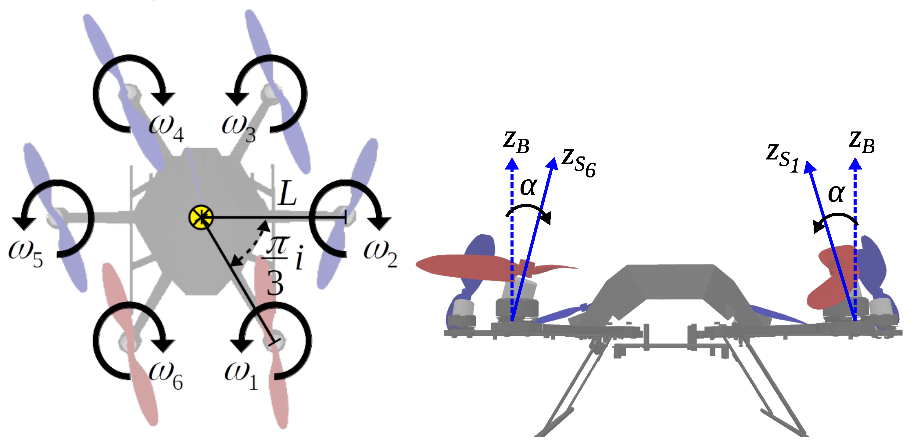
2.4. Dynamics of Omnidirectional Multirotor UAVs

Consider a fixed world frame ${\mathcal{F}}_W={\mathbf{O}}_W,\left\{{\mathbf{x}}_W,{\mathbf{y}}_W,{\mathbf{z}}_W\right\}$ and the body frame of the hexarotor ${\mathcal{F}}_b={\mathbf{O}}_b,\left\{{\mathbf{x}}_b,{\mathbf{y}}_b,{\mathbf{z}}_b\right\}$, which is attached to its center of mass (CoM), as well as six coordinate frames ${\mathcal{F}}_{S_i}={\mathbf{O}}_{S_i},\left\{{\mathbf{x}}_{S_i},{\mathbf{y}}_{S_i},{\mathbf{z}}_{S_i}\right\},i=1,\cdots ,6$, which are attached to each propeller of the hexarotor [27]. All of these frames are illustrated in Figure 1. The pose of the airframe with respect to ${\mathcal{F}}_W$ is represented by

$$\begin{array}{c}\hfill {\mathbf{p}}_b={\left[\begin{array}{ccc}x& y& z\end{array}\right]}^T\in {\mathbb{R}}^3,\end{array}$$

(14)

$$\begin{array}{c}\hfill {\mathsf{\eta }}_b={\left[\begin{array}{ccc}\varphi & \theta & \psi \end{array}\right]}^T\in {\mathbb{R}}^3,\end{array}$$

(15)

where $x,y,z\in \mathbb{R}$ are the Cartesian coordinates of translational motion representing the position of ${\mathcal{F}}_b$ in ${\mathcal{F}}_W$, and $\varphi ,\theta ,\psi \in \mathbb{R}$ are the Euler orientation angles about ${\mathbf{x}}_b$, ${\mathbf{y}}_b$, and ${\mathbf{z}}_b$, respectively. The orientation of ${\mathcal{F}}_b$ with respect to ${\mathcal{F}}_W$ is given by the rotation matrix ${\mathbf{R}}_b\in \mathrm{SO}(3)$, whose expression is given below:

$$\begin{array}{c}\hfill {\mathbf{R}}_b({\mathsf{\eta }}_b)=\left[\begin{array}{ccc}{c}_{\psi }{c}_{\theta }& c_{\psi }{s}_{\theta }{s}_{\varphi }-s_{\psi }{c}_{\varphi }& c_{\psi }{s}_{\theta }{c}_{\varphi }+s_{\psi }{s}_{\varphi }\\ s_{\psi }{c}_{\theta }& s_{\psi }{s}_{\theta }{s}_{\varphi }+c_{\psi }{c}_{\varphi }& s_{\psi }{s}_{\theta }{c}_{\varphi }-c_{\psi }{s}_{\varphi }\\ -s_{\theta }& c_{\theta }{s}_{\varphi }& c_{\theta }{c}_{\varphi }\end{array}\right],\end{array}$$

(16)

where $c_{(·)}\triangleq cos(·)$ and $s_{(·)}\triangleq sin(·)$. Let ${\dot{\mathbf{p}}}_b\in {\mathbb{R}}^3$ denote the absolute translational velocity of the UAV expressed in ${\mathcal{F}}_W$, while ${\dot{\mathsf{\eta }}}_b\in {\mathbb{R}}^3$ is the time derivative of ${\mathsf{\eta }}_b$. Then, the dynamics of an omnidirectional multirotor UAV can be written as [28]:

$$m{\ddot{\mathbf{p}}}_b=mg{\mathbf{e}}_3+{\mathbf{R}}_b({\mathsf{\eta }}_b){\mathbf{u}}_f+{\mathbf{f}}_u(·),$$

(17)

$$\mathbf{M}({\mathsf{\eta }}_b){\ddot{\mathsf{\eta }}}_b=-\mathbf{C}({\mathsf{\eta }}_b,{\dot{\mathsf{\eta }}}_b){\dot{\mathsf{\eta }}}_b+\Omega {({\mathsf{\eta }}_b)}^T{\mathbf{u}}_{\tau }+{\mathsf{\tau }}_u(·),$$

(18)

where $m>0$ is a scalar denoting the total mass of the UAV, g is a scalar representing the gravity acceleration, ${\mathbf{e}}_3={\left[001\right]}^T$, ${\mathbf{u}}_f,{\mathbf{u}}_{\tau }\in {\mathbb{R}}^3$ are the control forces and torque vectors, respectively, ${\mathbf{f}}_u(·),{\mathsf{\tau }}_u(·)\in {\mathbb{R}}^3$ represent the external forces and torques, respectively,

$$\Omega ({\mathsf{\eta }}_b)=\left[\begin{array}{ccc}1& 0& -s_{\theta }\\ 0& c_{\varphi }& c_{\theta }{s}_{\varphi }\\ 0& -s_{\varphi }& c_{\theta }{c}_{\varphi }\end{array}\right],$$

$\mathbf{M}({\mathsf{\eta }}_b)\in {\mathbb{R}}^{3\times 3}=\Omega {({\mathsf{\eta }}_b)}^T{\mathit{I}}_b\Omega ({\mathsf{\eta }}_b)$ with ${\mathit{I}}_b\in {\mathbb{R}}^{3\times 3}$ representing the inertia tensor of the UAV, and

$$\begin{array}{c}\hfill \mathbf{C}({\mathsf{\eta }}_b,{\dot{\mathsf{\eta }}}_b)\in {\mathbb{R}}^{3\times 3}=\Omega {({\mathsf{\eta }}_b)}^T{\left[\Omega ({\mathsf{\eta }}_b){\dot{\mathsf{\eta }}}_b\right]}_{\times }{\mathit{I}}_b\Omega ({\mathsf{\eta }}_b)+\Omega {({\mathsf{\eta }}_b)}^T{\mathit{I}}_b\dot{\Omega }({\mathsf{\eta }}_b),\end{array}$$

with ${[·]}_{\times }$ denoting the skew symmetric matrix. Considering the state $\overline{\mathbf{x}}={[\underset{{\mathbf{x}}_1}{\underbrace{{\mathbf{p}}_b^T{\mathsf{\eta }}_b^T}}\underset{{\mathbf{x}}_2}{\underbrace{{\dot{\mathbf{p}}}_b^T{\dot{\mathsf{\eta }}}_b^T}}]}^T$, the dynamics (17)–(18) can be rewritten as:

$$\dot{\overline{\mathbf{x}}}=\mathbf{A}\overline{\mathbf{x}}+\mathbf{B}({\mathsf{\eta }}_b)\mathbf{u}+\left[\begin{array}{c}{\mathbf{0}}_6\\ {\mathsf{\delta }}_1({\mathsf{\eta }}_b,{\dot{\mathsf{\eta }}}_b,g)+{\mathsf{\delta }}_2(·)\end{array}\right],$$

(19)

where

$$\mathbf{A}\in {\mathbb{R}}^{12\times 12}\triangleq \left[\begin{array}{cc}{\mathbf{O}}_{6\times 6}& {\mathbf{I}}_{6\times 6}\\ {\mathbf{O}}_{6\times 6}& {\mathbf{O}}_{6\times 6}\end{array}\right],$$

$$\mathbf{B}({\mathsf{\eta }}_b)\in {\mathbb{R}}^{12\times 6}\triangleq \left[\begin{array}{c}\underset{{\mathbf{B}}_1}{\underbrace{{\mathit{O}}_{6\times 6}}}\\ \underset{{\mathbf{B}}_2}{\underbrace{{\left[\begin{array}{cc}m{\mathbf{I}}_{3\times 3}& {\mathit{O}}_{3\times 3}\\ {\mathit{O}}_{3\times 3}& \mathbf{M}({\mathsf{\eta }}_b)\end{array}\right]}^{-1}\left[\begin{array}{cc}{\mathbf{R}}_b({\mathsf{\eta }}_b)& {\mathit{O}}_{3\times 3}\\ {\mathit{O}}_{3\times 3}& \Omega ({\mathsf{\eta }}_b)\end{array}\right]}}\end{array}\right].$$

$\mathbf{B}({\mathsf{\eta }}_b)$ is hereafter denoted as $\mathbf{B}$ for brevity; besides, ${\mathit{O}}_{n\times m}\in {\mathbb{R}}^{n\times m}$ is the zero matrix of proper dimensions, ${\mathit{I}}_{n\times m}\in {\mathbb{R}}^{n\times m}$ is the identity matrix of proper dimensions, $\mathbf{u}={[{\mathbf{u}}_f^T{\mathbf{u}}_{\tau }^T]}^T$ is a six-dimensional control vector,

$${\mathsf{\delta }}_1({\mathsf{\eta }}_b,{\dot{\mathsf{\eta }}}_b,g)\in {\mathbb{R}}^6\triangleq {\mathbf{B}}_2^{-1}{\left[\begin{array}{cc}-g{\mathbf{e}}_3^T& {(-\mathbf{C}({\mathsf{\eta }}_b,{\dot{\mathsf{\eta }}}_b){\dot{\mathsf{\eta }}}_b)}^T\end{array}\right]}^T$$

(20)

is the vector containing the gravity and Coriolis effects (which are considered as disturbance terms), and ${\mathsf{\delta }}_2(·)\in {\mathbb{R}}^6\triangleq {\left[{\mathbf{f}}_u{(·)}^T{\tau }_u{(·)}^T\right]}^T$ is the lumped vector of disturbances, including both external effects and the net term caused by parametric uncertainty. The term ${\mathsf{\delta }}_2(·)$ is typically unknown but bounded, $\parallel {\mathsf{\delta }}_2(·)\parallel \le {\gamma }_{{\mathsf{\delta }}_2}<+\infty$, and it is differentiable or at least has a removable discontinuity such that its time derivative is also bounded, $\parallel {\dot{\mathsf{\delta }}}_2(·)\parallel \le {\gamma }_{{\dot{\delta }}_2}<+\infty$. The following assumptions can also be made about (19):

A1.

The aerial vehicle does not pass through singularities [28]. In addition, it moves using the thrust incoming from the tilted propellers rather than changing its orientation to generate a thrust to move horizontally. In addition, it takes off with zero roll and pitch, and it is desired to maintain such values. Thus, the matrix ${\mathbf{B}}_2$ can be considered invertible.

A2.

Since ${\mathbf{B}}_2$ is invertible within some range and its norm is bounded (such a matrix is composed of the mass matrix, which is bounded for mechanical systems, a rotation matrix, and $\Omega (·)$, whose norms are bounded because they are composed of sine and cosine terms), $\mathbf{C}(\mathsf{\eta },\dot{\mathsf{\eta }})$ is Lipschitz continuous, and it does not grow faster than its arguments [29]. Hence, the following bounds hold:

$$\begin{array}{cc}\hfill & \parallel {\mathsf{\delta }}_1({\mathsf{\eta }}_b,{\dot{\mathsf{\eta }}}_b,g)\parallel \le {\gamma }_{{\delta }_1}\hfill \end{array}$$

(21)

$$\begin{array}{cc}\hfill & \parallel {\dot{\mathsf{\delta }}}_1({\mathsf{\eta }}_b,{\dot{\mathsf{\eta }}}_b,g)\parallel \le {\gamma }_{{\dot{\delta }}_1},\hfill \end{array}$$

(22)

with ${\gamma }_{{\delta }_1},{\gamma }_{{\dot{\delta }}_1}>0$.

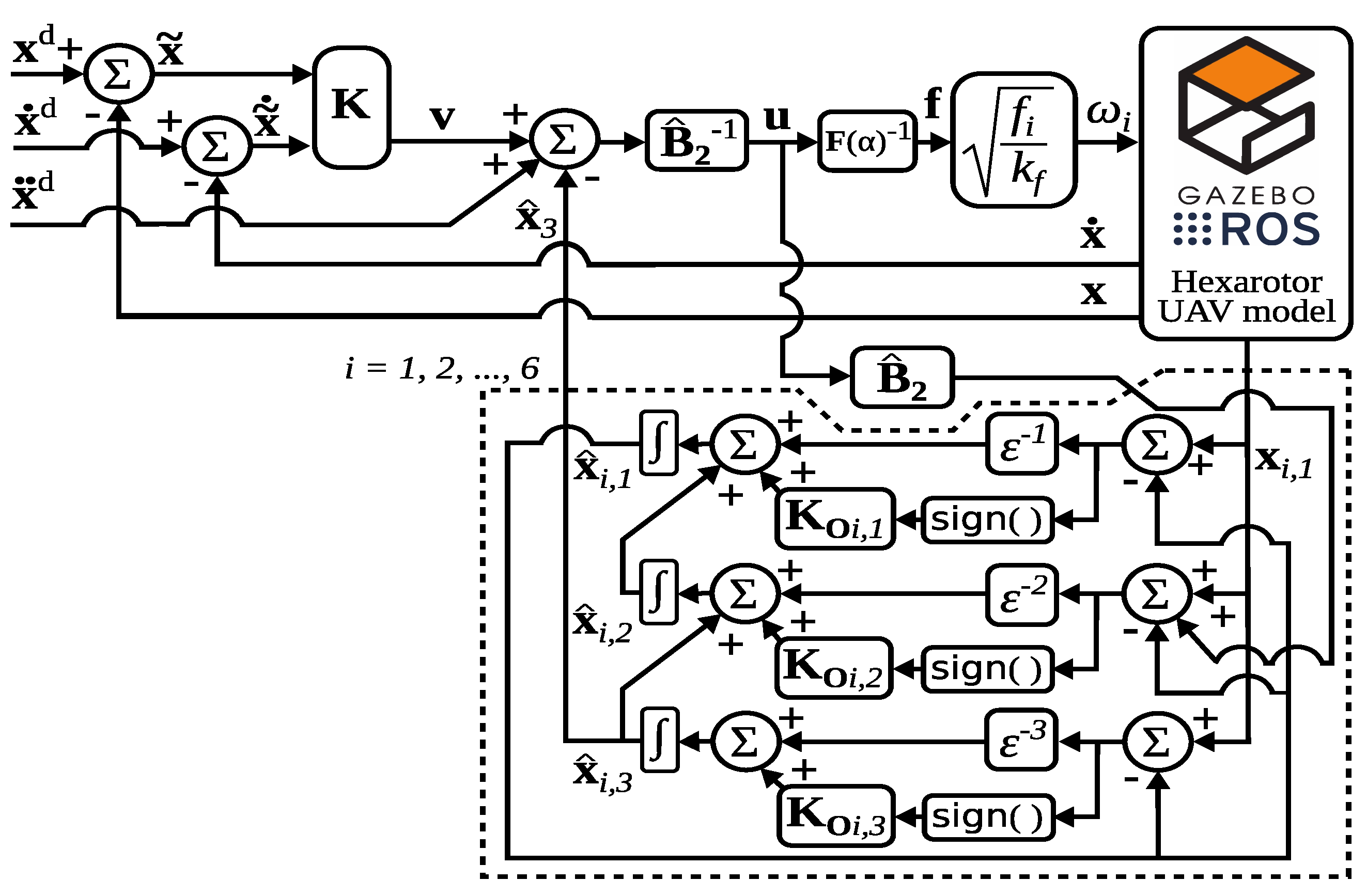
3. Controller Design

3.1. Control Problem

Consider the passively tilted hexarotor dynamics (19). The control problem is to lead ${\left[{\mathbf{x}}_1^T{\mathbf{x}}_2^T\right]}^T\in {\mathbb{R}}^{12}$ to the desired set point or trajectory ${[{{\mathbf{x}}_1^d}^T{{\mathbf{x}}_2^d}^T]}^T\in {\mathbb{R}}^{12}$ despite the disturbances affecting it. An appropriate solution is

$$\mathbf{u}={\mathbf{B}}_2^{-1}\left[\mathbf{v}-{\mathsf{\delta }}_1({\mathsf{\eta }}_b,{\dot{\mathsf{\eta }}}_b,g)-{\mathsf{\delta }}_2(·)\right],$$

(23)

where $\mathbf{v}\in {\mathbb{R}}^6$ is a virtual linear control input that can be shaped through any pole placement technique—for instance,

$$\mathbf{v}=\mathbf{K}\left[\begin{array}{c}{\tilde{\mathbf{x}}}_1\\ {\tilde{\mathbf{x}}}_2\end{array}\right],$$

(24)

where

$$\left[\begin{array}{c}{\tilde{\mathbf{x}}}_1\\ {\tilde{\mathbf{x}}}_2\end{array}\right]\in {\mathbb{R}}^{12}=\left[\begin{array}{c}{\mathbf{x}}_1^d\\ {\mathbf{x}}_2^d\end{array}\right]-\left[\begin{array}{c}{\mathbf{x}}_1\\ {\mathbf{x}}_2\end{array}\right]$$

is the error signal and $\mathbf{K}\in {\mathbb{R}}^{6\times 12}$ is a constant gain matrix. For the ideal case when the dynamics of the UAV are completely known, all of the states are measurable, and the external disturbances are absent (i.e., ${\dot{\mathsf{\delta }}}_2(·)={\mathbf{0}}_6$), the controller (23) is enough to solve the control problem, since ${\mathsf{\delta }}_1({\mathsf{\eta }}_b,{\dot{\mathsf{\eta }}}_b,g)$ is also known. On the other hand, external disturbances ${\mathsf{\delta }}_2(·)$ are usually unknown but bounded. Hence, when the UAV is affected by them, a control action to compensate for their effect is required. Below, the rejection of disturbances affecting (19) is explained—the technique consists of estimating and compensating online the total disturbance using a robust extended-state observer. The following two cases are presented: The former considers the external disturbance rejection via an extended-state observer and perfect cancellation of ${\mathsf{\delta }}_1(·)$; in the latter, such a vector is estimated as well.

3.2. External Disturbance Rejection via the Extended-State Observer and Perfect Cancellation of System Nonlinearities

Usually, the ADRC theory requests the knowledge of some boundaries for the total disturbance lumped within an additional state from the original system. In such a case, several types of extended-state observers have been implemented, including, recently, sliding-mode approaches. For the case of passively tilted hexarotors, this theory has not been applied. The closest works are about the application of ADRC to coplanar (non-tilted) hexarotors [3,4], but the convergence of the observers is missing. Below, the convergence of the sliding-mode extended-state observer and the ADRC based on such an observation technique is presented. For the control design, the fully actuated multirotor UAV subjected to the external disturbances in (19) can be rewritten in the following extended-state form:

$$\left\{\begin{array}{c}{\dot{\mathbf{x}}}_1={\mathbf{x}}_2,\hfill \\ {\dot{\mathbf{x}}}_2={\mathbf{B}}_2\mathbf{u}+{\mathsf{\delta }}_1({\mathsf{\eta }}_b,{\dot{\mathsf{\eta }}}_b,g)+{\mathbf{x}}_3,\hfill \\ {\dot{\mathbf{x}}}_3={\dot{\mathsf{\delta }}}_2(·).\hfill \end{array}\right.$$

(25)

Assuming an accurate knowledge of the parameters of the UAV dynamics (25) and an accurate measure of ${\mathbf{x}}_1$ and ${\mathbf{x}}_2$ (the vector ${\mathbf{x}}_2$ could be, in principle, estimated), a controller that satisfies set-point regulation and tracking is the following ADRC:

$$\mathbf{u}={\mathbf{B}}_2^{-1}\left[\mathbf{v}-{\mathsf{\delta }}_1({\mathsf{\eta }}_b,{\dot{\mathsf{\eta }}}_b,g)-{\widehat{\mathbf{x}}}_3+{\dot{\mathbf{x}}}_2^d\right],$$

(26)

from which ${\widehat{\mathbf{x}}}_3$ can be retrieved through the following robust SMESO:

$$\left\{\begin{array}{cc}\hfill {\dot{\widehat{\mathbf{x}}}}_1=& {\widehat{\mathbf{x}}}_2+{\epsilon }^{-1}({\mathbf{x}}_1-{\widehat{\mathbf{x}}}_1)+k_1\mathrm{sign}({\mathbf{x}}_1-{\widehat{\mathbf{x}}}_1)\hfill \\ \hfill {\dot{\widehat{\mathbf{x}}}}_2=& {\widehat{\mathbf{x}}}_3+{\epsilon }^{-2}({\mathbf{x}}_1-{\widehat{\mathbf{x}}}_1)+k_2\mathrm{sign}({\mathbf{x}}_1-{\widehat{\mathbf{x}}}_1)+{\mathbf{B}}_2\mathbf{u}+{\mathsf{\delta }}_1({\mathsf{\eta }}_b,{\dot{\mathsf{\eta }}}_b,g)\hfill \\ \hfill {\dot{\widehat{\mathbf{x}}}}_3=& {\epsilon }^{-3}({\mathbf{x}}_1-{\widehat{\mathbf{x}}}_1)+k_3\mathrm{sign}({\mathbf{x}}_1-{\widehat{\mathbf{x}}}_1),\hfill \end{array}\right.$$

(27)

where ${\widehat{\mathbf{x}}}_i\in {\mathbb{R}}^6$ contains the estimation of ${\mathbf{x}}_i$, $0<\epsilon \ll 1$ is a scalar such that the polynomial $s^3+{\epsilon }^{-1}{s}^2+{\epsilon }^{-2}s+{\epsilon }^{-3}$ is Hurwitz, and $k_1,k_2,k_3$ are positive scalars satisfying ${\epsilon }^{-1}>k_3>k_2>k_1>{\gamma }_{{\dot{\delta }}_2}$.

The boundedness of the estimation and the tracking errors are now shown in the following theorems.

Theorem 1.

The external disturbances ${\mathsf{\delta }}_2(·)$ are accurately reconstructed by the extended robust SMESO (27), i.e., the observation error $\widehat{\tilde{\mathbf{x}}}=\mathbf{x}-\widehat{\mathbf{x}}\in {\mathbb{R}}^{18}$ is uniformly ultimately bounded.

Proof of Theorem 1. 

Considering (25), the dynamics of the SMESO (27) are

$$\begin{array}{cc}\hfill \dot{\widehat{\tilde{\mathbf{x}}}}\triangleq \left[\begin{array}{c}{\dot{\widehat{\tilde{\mathbf{x}}}}}_1\\ {\dot{\widehat{\tilde{\mathbf{x}}}}}_2\\ {\dot{\widehat{\tilde{\mathbf{x}}}}}_3\end{array}\right]& =\underset{\tilde{\mathbf{A}}}{\underbrace{\left[\begin{array}{ccc}-{\epsilon }^{-1}{\mathbf{I}}_{6\times 6}& {\mathbf{I}}_{6\times 6}& {\mathbf{0}}_{6\times 6}\\ -{\epsilon }^{-2}{\mathbf{I}}_{6\times 6}& {\mathit{O}}_{6\times 6}& {\mathbf{I}}_{6\times 6}\\ -{\epsilon }^{-3}{\mathbf{I}}_{6\times 6}& {\mathit{O}}_{6\times 6}& {\mathit{O}}_{6\times 6}\end{array}\right]}}\underset{\widehat{\tilde{\mathbf{x}}}}{\underbrace{\left[\begin{array}{c}{\widehat{\tilde{\mathbf{x}}}}_1\\ {\widehat{\tilde{\mathbf{x}}}}_2\\ {\widehat{\tilde{\mathbf{x}}}}_3\end{array}\right]}}-\underset{{\mathbf{K}}_{\mathbf{O}}}{\underbrace{\left[\begin{array}{ccc}{k}_1{\mathbf{I}}_{6\times 6}& {\mathit{O}}_{6\times 6}& {\mathit{O}}_{6\times 6}\\ {\mathit{O}}_{6\times 6}& k_2{\mathbf{I}}_{6\times 6}& {\mathit{O}}_{6\times 6}\\ {\mathit{O}}_{6\times 6}& {\mathit{O}}_{6\times 6}& k_3{\mathbf{I}}_{6\times 6}\end{array}\right]}}\mathrm{sign}({\widehat{\tilde{\mathbf{x}}}}_1)\hfill \\ & +\underset{{\mathbf{D}}_1}{\underbrace{\left[\begin{array}{c}{\mathit{O}}_{6\times 6}\\ {\mathit{O}}_{6\times 6}\\ {\mathbf{I}}_{6\times 6}\end{array}\right]}}{\dot{\mathsf{\delta }}}_2(·)\hfill \end{array}$$

Considering the linear system $\dot{\widehat{\tilde{\mathbf{x}}}}=\tilde{\mathbf{A}}\widehat{\tilde{\mathbf{x}}}$, since $\tilde{\mathbf{A}}$ is Hurwitz, there exists a symmetric positive definite matrix ${\tilde{\mathbf{P}}}_1\in {\mathbb{R}}^{18\times 18}$ such that ${\tilde{\mathbf{A}}}^T{\tilde{\mathbf{P}}}_1+{\tilde{\mathbf{P}}}_1\tilde{\mathbf{A}}=-2{\mathbf{I}}_{18\times 18}$, and hence, a candidate Lyapunov function $V_1(\widehat{\tilde{\mathbf{x}}})={\widehat{\tilde{\mathbf{x}}}}^T{\tilde{\mathbf{P}}}_1\widehat{\tilde{\mathbf{x}}}$ can be proposed. Notice that such a function satisfies (8):

$${\lambda }_{\min }({\tilde{\mathbf{P}}}_1){\parallel \mathbf{x}\parallel }^2\le V_1(\widehat{\tilde{\mathbf{x}}})\le {\lambda }_{\max }({\tilde{\mathbf{P}}}_1){\parallel \mathbf{x}\parallel }^2.$$

In addition, the conditions (9) and (10) are satisfied with $c_3=2$ and $c_4=2{\lambda }_{\max }({\tilde{\mathbf{P}}}_1)$, respectively.

Now, considering the full system $\dot{\widehat{\tilde{\mathbf{x}}}}=\tilde{\mathbf{A}}\widehat{\tilde{\mathbf{x}}}-{\mathbf{K}}_o\mathrm{sign}({\widehat{\tilde{\mathbf{x}}}}_1)+{\mathbf{D}}_1{\dot{\mathsf{\delta }}}_2(·)$, Lemma 1 must be followed with the position $\rho =+\infty$. Therefore, the following ultimate bound can be proved:

$$-\parallel {\mathbf{K}}_o\mathrm{sign}({\widehat{\tilde{\mathbf{x}}}}_1)\parallel +\parallel {\mathbf{D}}_1{\dot{\mathsf{\delta }}}_2(·)\parallel \le -\sqrt{6}{k}_3+{\gamma }_{{\dot{\delta }}_2}<+\infty .$$

Hence, the solution of the SMESO system satisfies the following bounds:

$$\parallel \widehat{\tilde{\mathbf{x}}}(t)\parallel \le \left\{\begin{array}{c}\hfill \sqrt{{\displaystyle \frac{{\lambda }_{\max }({\tilde{\mathbf{P}}}_1)}{{\lambda }_{\min }({\tilde{\mathbf{P}}}_1)}}}\exp \left[-{\displaystyle \frac{(1-{\vartheta }_1)}{{\lambda }_{\max }({\tilde{\mathbf{P}}}_1)}}(t-t_0)\right]\parallel \widehat{\tilde{\mathbf{x}}}(0)\parallel ,\forall t_0\le t<t_1\\ \\ b_1,\forall t\ge t_1,\hfill \end{array}\right.$$

with $0<{\vartheta }_1<1$ and where

$$b_1={\displaystyle \frac{{\lambda }_{\max }({\tilde{\mathbf{P}}}_1)\left[{\gamma }_{{\dot{\delta }}_2}-\sqrt{6}{k}_3\right]}{{\vartheta }_1}}\sqrt{{\displaystyle \frac{{\lambda }_{\max }({\tilde{\mathbf{P}}}_1)}{{\lambda }_{\min }({\tilde{\mathbf{P}}}_1)}}}.$$

Notice that the gain $k_3$ is helpful for reducing the ultimate bound for the solutions of $\widehat{\tilde{\mathbf{x}}}$. □

Theorem 2.

The error vector ${\left[{\tilde{\mathbf{x}}}_1^T{\tilde{\mathbf{x}}}_2^T\right]}^T\in {\mathbb{R}}^{12}\triangleq {\left[{{\mathbf{x}}_1^d}^T{{\mathbf{x}}_2^d}^T\right]}^T-{\left[{\mathbf{x}}_1^T{\mathbf{x}}_2^T\right]}^T$, with ${\dot{\mathbf{x}}}_1^d={\mathbf{x}}_2^d$, is uniformly ultimately bounded by means of the controller (26).

Proof of Theorem 2. 

Considering (25), the tracking error dynamics are

$$\left\{\begin{array}{c}{\dot{\tilde{\mathbf{x}}}}_1={\tilde{\mathbf{x}}}_2,\hfill \\ \hfill {\dot{\tilde{\mathbf{x}}}}_2={\dot{\mathbf{x}}}_2^d-{\mathbf{B}}_2\mathbf{u}-{\mathsf{\delta }}_1({\mathsf{\eta }}_b,{\dot{\mathsf{\eta }}}_b,g)-{\mathbf{x}}_3.\end{array}\right.$$

Substituting the controller (26) into the error dynamics yields

$$\left\{\begin{array}{c}{\dot{\tilde{\mathbf{x}}}}_1={\tilde{\mathbf{x}}}_2,\hfill \\ \hfill {\dot{\tilde{\mathbf{x}}}}_2=-\mathbf{v}+{\widehat{\mathbf{x}}}_3-{\mathbf{x}}_3.\end{array}\right.$$

Considering ${\widehat{\mathbf{x}}}_3-{\mathbf{x}}_3=-{\widehat{\tilde{\mathbf{x}}}}_3$, then

$$\left[\begin{array}{c}{\dot{\tilde{\mathbf{x}}}}_1\\ {\dot{\tilde{\mathbf{x}}}}_2\end{array}\right]=\left[\begin{array}{cc}{\mathit{O}}_{6\times 6}& {\mathbf{I}}_{6\times 6}\\ {\mathit{O}}_{6\times 6}& {\mathit{O}}_{6\times 6}\end{array}\right]\left[\begin{array}{c}{\tilde{\mathbf{x}}}_1\\ {\tilde{\mathbf{x}}}_2\end{array}\right]-\left[\begin{array}{c}{\mathit{O}}_{6\times 6}\\ {\mathbf{I}}_{6\times 6}\end{array}\right]\mathbf{v}-\left[\begin{array}{c}{\mathit{O}}_{6\times 6}\\ {\mathbf{I}}_{6\times 6}\end{array}\right]{\widehat{\tilde{\mathbf{x}}}}_3.$$

Folding (23) into the last expression yields

$$\left[\begin{array}{c}{\dot{\tilde{\mathbf{x}}}}_1\\ {\dot{\tilde{\mathbf{x}}}}_2\end{array}\right]={\mathbf{A}}_1\left[\begin{array}{c}{\tilde{\mathbf{x}}}_1\\ {\tilde{\mathbf{x}}}_2\end{array}\right]-\left[\begin{array}{c}{\mathit{O}}_{6\times 6}\\ {\mathbf{I}}_{6\times 6}\end{array}\right]{\widehat{\tilde{\mathbf{x}}}}_3,$$

with

$${\mathbf{A}}_1=\left[\begin{array}{cc}{\mathit{O}}_{6\times 6}& {\mathbf{I}}_{6\times 6}\\ {\mathit{O}}_{6\times 6}& {\mathit{O}}_{6\times 6}\end{array}\right]-\left[\begin{array}{c}{\mathit{O}}_{6\times 6}\\ {\mathbf{I}}_{6\times 6}\end{array}\right]\mathbf{K},$$

such that $\mathbf{K}$ makes ${\mathbf{A}}_1$ Hurwitz.

Considering the nominal linear system with ${\widehat{\tilde{\mathbf{x}}}}_3={\mathbf{0}}_6$, a candidate Lyapunov function $V_2({\tilde{\mathbf{x}}}_1,{\tilde{\mathbf{x}}}_2)=$${\left[{\tilde{\mathbf{x}}}_1^T{\tilde{\mathbf{x}}}_2^T\right]}^T{\mathbf{P}}_1\left[{\tilde{\mathbf{x}}}_1^T{\tilde{\mathbf{x}}}_2^T\right]$ can be proposed, where ${\mathbf{P}}_1\in {\mathbb{R}}^{12\times 12}$ is a symmetric positive definite matrix that is solution of

$${\mathbf{A}}_1^T{\mathbf{P}}_1+{\mathbf{P}}_1{\mathbf{A}}_{\mathbf{1}}=-2{\mathbf{I}}_{12\times 12}.$$

Notice that such a function satisfies (8):

$${\lambda }_{\min }({\mathbf{P}}_1){\parallel \mathbf{x}\parallel }^2\le V_2(\widehat{\tilde{\mathbf{x}}})\le {\lambda }_{\max }({\mathbf{P}}_1){\parallel \mathbf{x}\parallel }^2.$$

Moreover, the conditions (9) and (10) are satisfied with $c_3=2$ and $c_4=2{\lambda }_{\max }({\mathbf{P}}_1)$, respectively. Now, considering the full system with the generic condition ${\widehat{\tilde{\mathbf{x}}}}_3\ne {\mathbf{0}}_6$, Lemma 1 must be followed with the position $\rho =+\infty$. The ultimate bound for ${\widehat{\tilde{\mathbf{x}}}}_3$ can be retrieved from Theorem 1. Thus, the solutions of the tracking error dynamics are uniformly ultimately bounded by

$$\left|\left|\left[\begin{array}{c}{\tilde{\mathbf{x}}}_1(t)\\ {\tilde{\mathbf{x}}}_2(t)\end{array}\right]\right|\right|\le \left\{\begin{array}{c}\hfill \sqrt{{\displaystyle \frac{{\lambda }_{\max }({\mathbf{P}}_1)}{{\lambda }_{\min }({\mathbf{P}}_1)}}}\exp \left[-{\displaystyle \frac{(1-{\vartheta }_2)}{{\lambda }_{\max }({\mathbf{P}}_1)}}(t-t_0)\right]\left|\left|\left[\begin{array}{c}{\tilde{\mathbf{x}}}_1(0)\\ {\tilde{\mathbf{x}}}_2(0)\end{array}\right]\right|\right|,\forall t_0\le t<t_2\\ \\ b_2,\forall t\ge t_2,\hfill \end{array}\right.$$

where

$$b_2={\displaystyle \frac{b_1{\lambda }_{\max }({\mathbf{P}}_1)}{{\vartheta }_2}}\sqrt{{\displaystyle \frac{{\lambda }_{\max }({\mathbf{P}}_1)}{{\lambda }_{\min }({\mathbf{P}}_1)}}},$$

and $t_2>t_1$. Notice that the ultimate bound $b_2$ depends directly on $b_1$. □

3.3. Robust External Disturbance Rejection via the Extended-State Observer

In case the disturbances ${\mathsf{\delta }}_1({\mathsf{\eta }}_b,{\dot{\mathsf{\eta }}}_b,g),{\mathsf{\delta }}_2(·)$ are differentiable in their arguments and locally Lipschitz or at least have a removable discontinuity (for the case of external disturbances), an augmented-state representation for (19) can be used as follows:

$$\dot{\mathbf{x}}\triangleq \left\{\begin{array}{c}{\dot{\mathbf{x}}}_1={\mathbf{x}}_2\hfill \\ {\dot{\mathbf{x}}}_2={\mathbf{B}}_2\mathbf{u}+{\mathbf{x}}_3\hfill \\ {\dot{\mathbf{x}}}_3={\dot{\mathsf{\delta }}}_1({\mathsf{\eta }}_b,{\dot{\mathsf{\eta }}}_b,g)+{\dot{\mathsf{\delta }}}_2(·).\hfill \end{array}\right.$$

(28)

A controller that satisfies set-point regulation and tracking is the following ADRC:

$$\mathbf{u}={\mathbf{B}}_2^{-1}\left[\mathbf{v}-{\widehat{\mathbf{x}}}_3+{\dot{\mathbf{x}}}_2^d\right],$$

(29)

where $\mathbf{v}$ is the same as in (24). The difference with respect to (26) is the missing compensation for the term ${\mathsf{\delta }}_1(·)$. The estimate of ${\widehat{\mathbf{x}}}_3$ can be retrieved through the following robust SMESO:

$$\left\{\begin{array}{cc}\hfill {\dot{\widehat{\mathbf{x}}}}_1=& {\widehat{\mathbf{x}}}_2+{\epsilon }^{-1}({\mathbf{x}}_1-{\widehat{\mathbf{x}}}_1)+k_1\mathrm{sign}({\mathbf{x}}_1-{\widehat{\mathbf{x}}}_1),\hfill \\ \hfill {\dot{\widehat{\mathbf{x}}}}_2=& {\widehat{\mathbf{x}}}_3+{\epsilon }^{-2}({\mathbf{x}}_1-{\widehat{\mathbf{x}}}_1)+k_2\mathrm{sign}({\mathbf{x}}_1-{\widehat{\mathbf{x}}}_1)+{\mathbf{B}}_2\mathbf{u},\hfill \\ \hfill {\dot{\widehat{\mathbf{x}}}}_3=& {\epsilon }^{-3}({\mathbf{x}}_1-{\widehat{\mathbf{x}}}_1)+k_3\mathrm{sign}({\mathbf{x}}_1-{\widehat{\mathbf{x}}}_1).\hfill \end{array}\right.$$

(30)

The boundedness of the estimation and the tracking errors are now shown in the following theorems.

Theorem 3.

The disturbances of (25) are accurately reconstructed by the extended robust SMESO (30) despite the missing compensation for ${\mathsf{\delta }}_1({\mathsf{\eta }}_b,{\dot{\mathsf{\eta }}}_b,g)$, i.e., the observation error $\widehat{\tilde{\mathbf{x}}}=\mathbf{x}-\widehat{\mathbf{x}}\in {\mathbb{R}}^{18\times 18}$ is uniformly ultimately bounded.

Proof of Theorem 3. 

Taking into account (28), the dynamics of the SMESO (30) are

$$\begin{array}{cc}\hfill \dot{\widehat{\tilde{\mathbf{x}}}}\triangleq \left[\begin{array}{c}{\dot{\widehat{\tilde{\mathbf{x}}}}}_1\\ {\dot{\widehat{\tilde{\mathbf{x}}}}}_2\\ {\dot{\widehat{\tilde{\mathbf{x}}}}}_3\end{array}\right]& =\underset{\tilde{\mathbf{A}}}{\underbrace{\left[\begin{array}{ccc}-{\epsilon }^{-1}{\mathbf{I}}_{6\times 6}& {\mathbf{I}}_{6\times 6}& {\mathit{O}}_{6\times 6}\\ -{\epsilon }^{-2}{\mathbf{I}}_{6\times 6}& {\mathit{O}}_{6\times 6}& {\mathbf{I}}_{6\times 6}\\ -{\epsilon }^{-3}{\mathbf{I}}_{6\times 6}& {\mathit{O}}_{6\times 6}& {\mathit{O}}_{6\times 6}\end{array}\right]}}\underset{\widehat{\tilde{\mathbf{x}}}}{\underbrace{\left[\begin{array}{c}{\widehat{\tilde{\mathbf{x}}}}_1\\ {\widehat{\tilde{\mathbf{x}}}}_2\\ {\widehat{\tilde{\mathbf{x}}}}_3\end{array}\right]}}-\underset{{\mathbf{K}}_{\mathbf{O}}}{\underbrace{\left[\begin{array}{ccc}{k}_1{\mathbf{I}}_{6\times 6}& {\mathit{O}}_{6\times 6}& {\mathit{O}}_{6\times 6}\\ {\mathit{O}}_{6\times 6}& k_2{\mathbf{I}}_{6\times 6}& {\mathit{O}}_{6\times 6}\\ {\mathit{O}}_{6\times 6}& {\mathit{O}}_{6\times 6}& k_3{\mathbf{I}}_{6\times 6}\end{array}\right]}}\mathrm{sign}({\widehat{\tilde{\mathbf{x}}}}_1)\hfill \\ & +\underset{{\mathbf{D}}_1}{\underbrace{\left[\begin{array}{c}{\mathit{O}}_{6\times 6}\\ {\mathit{O}}_{6\times 6}\\ {\mathbf{I}}_{6\times 6}\end{array}\right]}}({\dot{\mathsf{\delta }}}_1(g,{\mathsf{\eta }}_b,{\dot{\mathsf{\eta }}}_b)+{\dot{\mathsf{\delta }}}_2(·)).\hfill \end{array}$$

Considering the linear system $\dot{\widehat{\tilde{\mathbf{x}}}}=\tilde{\mathbf{A}}\widehat{\tilde{\mathbf{x}}}$, since $\tilde{\mathbf{A}}$ is Hurwitz, there exists a symmetric positive definite matrix ${\tilde{\mathbf{P}}}_2\in {\mathbb{R}}^{18\times 18}$ such that ${\tilde{\mathbf{A}}}^T{\tilde{\mathbf{P}}}_2+{\tilde{\mathbf{P}}}_2\tilde{\mathbf{A}}=-2{\mathbf{I}}_{18\times 18}$, and hence, a candidate Lyapunov function $V_3(\widehat{\tilde{\mathbf{x}}})={\widehat{\tilde{\mathbf{x}}}}^T{\tilde{\mathbf{P}}}_2\widehat{\tilde{\mathbf{x}}}$ can be proposed. Notice that such a function satisfies (8)

$${\lambda }_{\min }({\tilde{\mathbf{P}}}_2){\parallel \mathbf{x}\parallel }^2\le V_3(\widehat{\tilde{\mathbf{x}}})\le {\lambda }_{\max }({\tilde{\mathbf{P}}}_2){\parallel \mathbf{x}\parallel }^2.$$

In addition, the conditions (9) and (10) are satisfied with $c_3=2$ and $c_4=2{\lambda }_{\max }({\tilde{\mathbf{P}}}_2)$, respectively. Now, with the full system

$$\dot{\widehat{\tilde{\mathbf{x}}}}=\tilde{\mathbf{A}}\widehat{\tilde{\mathbf{x}}}-{\mathbf{K}}_o\mathrm{sign}({\widehat{\tilde{\mathbf{x}}}}_1)+{\mathbf{D}}_1({\dot{\mathsf{\delta }}}_1({\mathsf{\eta }}_b,{\dot{\mathsf{\eta }}}_b)+{\dot{\mathsf{\delta }}}_2(·)),$$

Lemma 1 must be followed with the position $\rho =+\infty$. Therefore, taking into account (20) and A2, the following ultimate bound can be proved:

$$-\parallel {\mathbf{K}}_o\mathrm{sign}({\widehat{\tilde{\mathbf{x}}}}_1)\parallel +\parallel {\mathbf{D}}_1({\dot{\mathsf{\delta }}}_1({\mathsf{\eta }}_b,{\dot{\mathsf{\eta }}}_b)+{\dot{\mathsf{\delta }}}_2(·))\parallel \le -\sqrt{6}{k}_3+{\gamma }_{{\dot{\delta }}_1}+{\gamma }_{{\dot{\delta }}_2}<+\infty .$$

Hence, the solution of the SMESO system satisfies the following bounds:

$$\parallel \widehat{\tilde{\mathbf{x}}}(t)\parallel \le \left\{\begin{array}{c}\hfill \sqrt{{\displaystyle \frac{{\lambda }_{\max }({\tilde{\mathbf{P}}}_2)}{{\lambda }_{\min }({\tilde{\mathbf{P}}}_2)}}}\exp \left[-{\displaystyle \frac{(1-{\vartheta }_3)}{{\lambda }_{\max }({\tilde{\mathbf{P}}}_2)}}(t-t_0)\right]\parallel \widehat{\tilde{\mathbf{x}}}(0)\parallel ,\forall t_0\le t<t_1\\ \\ b_3,\forall t\ge t_1,\hfill \end{array}\right.$$

with $0<{\vartheta }_3<1$ and

$$b_3={\displaystyle \frac{{\lambda }_{\max }({\tilde{\mathbf{P}}}_2)\left[{\gamma }_{{\dot{\mathsf{\delta }}}_1}+{\gamma }_{{\dot{\delta }}_2}-\sqrt{6}{k}_3\right]}{{\vartheta }_3}}\sqrt{{\displaystyle \frac{{\lambda }_{\max }({\tilde{\mathbf{P}}}_2)}{{\lambda }_{\min }({\tilde{\mathbf{P}}}_2)}}}.$$

□

Theorem 4.

The error vector ${\left[{\tilde{\mathbf{x}}}_1^T{\tilde{\mathbf{x}}}_2^T\right]}^T$ is uniformly ultimately bounded by means of the controller (29).

Proof of the Theorem 4. 

Considering (28), the tracking error dynamics are

$$\left\{\begin{array}{c}{\dot{\tilde{\mathbf{x}}}}_1={\tilde{\mathbf{x}}}_2,\hfill \\ \hfill {\dot{\tilde{\mathbf{x}}}}_2={\dot{\mathbf{x}}}_2^d-{\mathbf{B}}_2\mathbf{u}-{\mathbf{x}}_3.\end{array}\right.$$

Substituting the controller (29) yields

$$\left\{\begin{array}{c}{\dot{\tilde{\mathbf{x}}}}_1={\tilde{\mathbf{x}}}_2,\hfill \\ \hfill {\dot{\tilde{\mathbf{x}}}}_2=-\mathbf{v}-{\widehat{\tilde{\mathbf{x}}}}_3.\end{array}\right.$$

The procedure follows the proof within Theorem 2, and for brevity, it is not reported here. However, it is worth noting that the ultimate bound for $\left|\left|\left[\begin{array}{c}{\tilde{\mathbf{x}}}_1(t)\\ {\tilde{\mathbf{x}}}_2(t)\end{array}\right]\right|\right|$ now depends on $b_3$ from Theorem 3. □

4. Controller Implementation

4.1. Control Allocation

Consider Figure 2, where the top and frontal views of the tilted multirotor with six actuators are presented. The position of the i-th propeller in ${\mathcal{F}}_B$ can be mathematically expressed as follows [30]:

$${\mathbf{p}}_{S_i}^b=L{\mathbf{R}}_z\left({\zeta }_i\right){\left[\begin{array}{ccc}1& 0& 0\end{array}\right]}^T,$$

(31)

where $i=1,\cdots ,n$ depends on the multirotor, $L>0$ is the distance between ${\mathit{O}}_{S_i}$ and ${\mathit{O}}_B$, and ${\mathbf{R}}_z\in \mathrm{SO}(3)$ is the canonical rotation matrix around the axis ${\left[\begin{array}{ccc}0& 0& 1\end{array}\right]}^T$ [31]. The orientation of ${\mathcal{F}}_{S_i}$ with respect to ${\mathcal{F}}_B$ is given by [27]:

$${\mathbf{R}}_{S_i}^b(\alpha )={\mathbf{R}}_z\left({\zeta }_i\right){\mathbf{R}}_x\left({(-1)}^{i-1}{\alpha }_i(t)\right)\in \mathrm{SO}(3),$$

(32)

where $i=1,\cdots ,n$, ${\alpha }_i(t)\in \left[-\pi /2,\pi /2\right]$ is the tilt angle of the propellers about ${\mathbf{x}}_{S_i}$, and ${\mathbf{R}}_x\in \mathrm{SO}(3)$ is the canonical rotation matrix around the axis ${\left[\begin{array}{ccc}1& 0& 0\end{array}\right]}^T$ [31]. For the case of passively tilting multirotors, $\alpha {(t)}_i={\alpha }_i$ is considered, and it has the same magnitude for each propeller, while ${(-1)}^{i-1}$ denotes the orientation tilt of each propeller. Figure 2 illustrates the geometric concepts of the length from the propeller to the UAV’s CoM and the separation angle between each rotor. Furthermore, the spin direction of each propeller is displayed, and a front view of the hexarotor is also presented, where the tilting angle ${\alpha }_i$ about the ${\mathbf{x}}_{S_i}$ can be appreciated. Each propeller supplies a thrust force applied in ${\mathit{O}}_{S_i}$ that, expressed in ${\mathcal{F}}_B$, appears as follows [27]:

$${\mathbf{f}}_{}=f_i{\mathbf{R}}_{S_i}^b(\alpha ){\left[\begin{array}{ccc}0& 0& 1\end{array}\right]}^T\in {\mathbb{R}}^3,$$

(33)

where $i=1,\cdots ,6$, $f_i=k_f{\omega }_i^2$ is the intensity of the force provided by the i-th angular velocity ${\omega }_i\in \mathbb{R}$, and $k_f>0$ is a constant parameter depending on the geometry of the propeller [32]. Simultaneously, the following drag torque is supplied by the propellers [27]:

$${\tau }_{b_i}={(-1)}^{i-1}\sigma {\mathbf{f}}_{b_i}{\mathbf{R}}_{S_i}^b(\alpha ){\left[\begin{array}{ccc}0& 0& 1\end{array}\right]}^T\in {\mathbb{R}}^3,$$

(34)

where $i=1,\cdots ,6$ and $\sigma =k_{\tau }/k_f$, with $k_{\tau }>0$, is a constant parameter depending on the geometry of the propeller, and ${(-1)}^{i-1}$ models its spin direction. The total thrust forces applied to the airframe expressed in ${\mathcal{F}}_W$ are represented by [30]:

$${\mathbf{f}}_T={\mathbf{R}}_b\sum _{i=1}^6{\mathbf{f}}_{b_i}={\mathbf{R}}_b{\mathbf{F}}_1(\mathsf{\alpha })\mathbf{f},$$

(35)

where $\mathsf{\alpha }\in {\mathbb{R}}^n$ contains the tilting angle of each rotor, $\mathbf{f}={\left[\begin{array}{cc}{f}_1& \cdots f_n\end{array}\right]}^T\in {\mathbb{R}}^n$ is the stacking vector of the propeller forces, and ${\mathbf{F}}_1\in {\mathbb{R}}^{3\times n}$ is a mapping matrix from the propeller forces to the airframe forces. Likewise, the total torques applied to the airframe expressed in ${\mathcal{F}}_B$ are [32]:

$${\mathsf{\tau }}_T=\sum _{i=n}^6\left(\left({\mathbf{p}}_{S_i}^b\times {\mathbf{f}}_{b_i}\right)+{\mathsf{\tau }}_{b_i}\right)={\mathbf{F}}_2(\mathsf{\alpha })\mathbf{f},$$

(36)

where × is the cross-product operator and ${\mathbf{F}}_2\in {\mathbb{R}}^{3\times n}$ is the mapping matrix from the propeller forces to the torques applied to the airframe. Hence, the full allocation matrix is given by

$$\mathbf{F}(\mathsf{\alpha })=k_f\left[\begin{array}{c}{\mathbf{F}}_1(\mathsf{\alpha })\\ {\mathbf{F}}_2(\mathsf{\alpha })\end{array}\right].$$

(37)

For the case of passively tilted hexarotors, it follows that

$${\mathbf{F}}_1(\mathsf{\alpha })=\left[\begin{array}{cccccc}{\displaystyle \frac{s_{\alpha }}{2}}& -s_{\alpha }& {\displaystyle \frac{s_{\alpha }}{2}}& -{\displaystyle \frac{s_{\alpha }}{2}}& -s_{\alpha }& -{\displaystyle \frac{s_{\alpha }}{2}}\\ {\displaystyle \frac{\sqrt{3}{s}_{\alpha }}{2}}& 0& -{\displaystyle \frac{\sqrt{3}{s}_{\alpha }}{2}}& {\displaystyle \frac{\sqrt{3}{s}_{\alpha }}{2}}& 0& -{\displaystyle \frac{\sqrt{3}{s}_{\alpha }}{2}}\\ c_{\alpha }& c_{\alpha }& c_{\alpha }& c_{\alpha }& c_{\alpha }& c_{\alpha }\end{array}\right]$$

$${\mathbf{F}}_2(\mathsf{\alpha })={\left[\begin{array}{ccc}{\displaystyle \frac{L{\sigma }_{\alpha }-\sigma s_{\alpha }}{2}}& {\displaystyle \frac{\sqrt{3}(L{c}_{\alpha }-\sigma s_{\alpha })}{2}}& -L{s}_{\alpha }-\sigma c_{\alpha }\\ {\displaystyle L{\sigma }_{\alpha }-\sigma s_{\alpha }}& 0& L{s}_{\alpha }+\sigma c_{\alpha }\\ {\displaystyle \frac{L{\sigma }_{\alpha }-\sigma s_{\alpha }}{2}}& -{\displaystyle \frac{\sqrt{3}(L{c}_{\alpha }-\sigma s_{\alpha })}{2}}& -L{s}_{\alpha }-\sigma c_{\alpha }\\ -{\displaystyle \frac{L{\sigma }_{\alpha }-\sigma s_{\alpha }}{2}}& -{\displaystyle \frac{\sqrt{3}(L{c}_{\alpha }-\sigma s_{\alpha })}{2}}& L{s}_{\alpha }+\sigma c_{\alpha }\\ {\displaystyle -L{\sigma }_{\alpha }+\sigma s_{\alpha }}& 0& -L{s}_{\alpha }-\sigma c_{\alpha }\\ -{\displaystyle \frac{L{\sigma }_{\alpha }-\sigma s_{\alpha }}{2}}& {\displaystyle \frac{\sqrt{3}(L{c}_{\alpha }-\sigma s_{\alpha })}{2}}& L{s}_{\alpha }+\sigma c_{\alpha }\end{array}\right]}^T$$

Notice that (37) is static and invertible; therefore, the mapping from the six-dimensional control $\mathbf{u}$ (29) to the actuators’ forces is

$${\mathbf{f}}_b=\mathbf{F}{(\mathsf{\alpha })}^{-1}\mathbf{u}.$$

(38)

Finally, the rotor velocities can be computed through

$${\omega }_i=\sqrt{{\displaystyle \frac{f_i}{k_f}}}.$$

(39)

4.2. Setup of the 3D Simulation

The Gazebo dynamic simulator was used to demonstrate the effectiveness of the proposed approach. In this context, control algorithms were developed in the C++ programming language using the Robotics Operating System (ROS) as middleware [33]. At the same time, the simulation of the flying platform was based on the RotorS library [34]; this library implements dynamic flying robot models and sensor plugins that are suitable for Gazebo in the ROS and are usable for developing custom controllers designed to be analogous to their real-world counterparts, so each simulation is almost identical to a real experiment. By default, only flat UAVs are available when using the RotorS software. Therefore, a custom tilted hexacopter was designed and modeled, taking the well-known AscTec firefly platform as an inspiration. A significant benefit of the RotorS library when used with different control and state estimation algorithms is the possibility to simulate UAV rotors with desired motor dynamics and characteristics. In this way, a new multi-copter model can be designed by grouping different rotor models together. Each rotor imported into the simulation scene can be controlled with a desired rotation velocity command, which is consistent with the proposed control approach and allocation. The robot’s local position and attitude are available through the ROS network to implement the closed control loop.

The system architecture is depicted in Figure 3, and it is discussed in the following. Two main modules were deployed in the form of ROS nodes: the controller (29) and the observer (30). The latter took the desired control signal generated by the controller and the multirotor’s full pose as inputs. At the same time, its output was represented by the estimation of the total disturbances acting on the platform. As for the controller, this module received the platform’s pose from the Gazebo simulator and the disturbance estimation provided by the observer to generate the six desired motor control signals, which were expressed in rpm (revolutions per minute). In this context,

Table 1. List of parameters used for the implementation of the controller and the aerial platform.

Parameter	Value
m	$2.1$ kg
${\mathbf{I}}_b$	$\mathrm{diag}(0.0347563,0.0458929,0.0977)$ kg m ${}^2$
${\omega }_{i_{max}}$	1500 rpm
$k_f$	$8.54858\times {10}^{-6}$
$k_{\tau }$	$1\times {10}^{-2}$
L	$0.215$ m
$\alpha$	20 deg
${\mathbf{K}}_{1,\cdots ,6}$	$\left\{2,2,20,800,800,2500\right\}$
${\mathbf{K}}_{7,\cdots ,12}$	$\left\{4,4,25,1200,1200,5000\right\}$

reports a list of the controller’s parameters and the characteristics of the UAV platform and its motors that were used test both the SMC and the ADRC. In particular, ${\omega }_{i_{max}}$ represents the maximum rotational velocity of the motors, $k_f$ and $k_{\tau }$ represent their drag force and rolling moment constants, respectively, L is the length of the UAV arm, and $\alpha$ is the tilt angle of each rotor. However, ${\mathbf{K}}_{1,\cdots ,6}$ and ${\mathbf{K}}_{7,\cdots ,12}$ are the main diagonal components of the feedback gain matrices. It is worth mentioning that the same proportional and derivative gains were used to test both controllers; the difference was in how they rejected disturbances, namely, SMC used the sliding term while ADRC used the observed signal of the augmented state as feedback. The system was tested on a standard computer running Ubuntu 20.04 as it operating system, while ROS Noetic was chosen as the distribution.

5. Case Studies

This section addresses the tests that were conducted to assess the effectiveness of the proposed control–observer scheme. First, a complex trajectory was commanded to evaluate the tracking performance; the following experiments consisted of a regulation task at a given pose in the presence of external disturbances, which were implemented using an external wrench plugin for Gazebo (https://github.com/Viviana-Morl/ft_gazebo_plugin (accessed on 4 August 2022)). Finally, a comparison of the proposed controller with a sliding-mode controller was carried out. All of the tests are shown in a video (https://www.youtube.com/watch?v=TyOvDe81VHc (accessed on 4 August 2022)).

5.1. Tracking

This test consisted of commanding to take a complex trajectory in Cartesian coordinates with respect to the world frame ${\mathcal{F}}_W$. The Cartesian position’s trajectory is given by the following parametric equations of a Lemniscate:

$$\left\{\begin{array}{c}{x}_b^d={\displaystyle \frac{acos(2\pi f_{t}t)}{1+{sin}^2(2\pi f_{t}t)}}\hfill \\ \\ y_b^d={\displaystyle \frac{asin(2\pi f_{t}t)cos(2\pi f_{t}t)}{1+{sin}^2(2\pi f_{t}t)}}\hfill \\ \\ z_b^d=bt\hfill \end{array}\right.,$$

(40)

where $a=1.4,b=0.2$ are scalar parameters, t is the time, and $f_t=0.5$ is the frequency in Hz. The time derivatives of (40) were computing numerically. Firstly, the UAV was commanded to take off; thereafter, it was commanded to reach $(x_b^d,y_b^d,z_b^d)=(0,1.4,1)$ m with zero orientation so that it could start and then perform the lemniscate trajectory; finally, it was commanded to end by hovering steadily.

Figure 4 shows the norm of the state error $\parallel \tilde{\mathbf{x}}\parallel$ during the whole experiment. It can be seen that this norm was always below 3 cm when the UAV was flying and decreased to zero when it hovered. Furthermore, Figure 5 displays that the UAV trajectory tracked the desired trajectory in the Cartesian space.

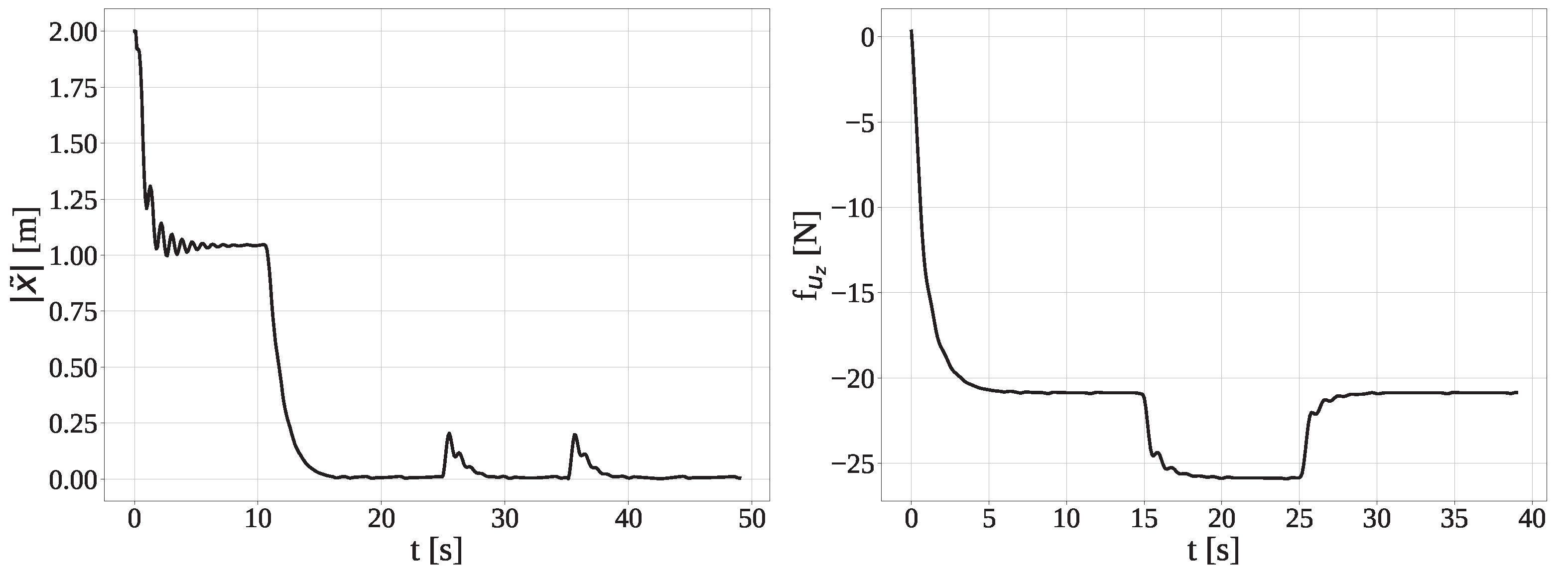
5.2. Regulation with Wind and Payload

The robustness of the observer–controller scheme was assessed by simulating wind conditions while the UAV was hovering at a target set point. The first experiment involved flying the UAV to the set point $(x_b^d,y_b^d,z_b^d)=(1,1,2)$ m with zero orientation and applying an external disturbance a few seconds after it reached the set point. This disturbance represented a sudden wind shear given by

$${\mathbf{f}}_u=\left[\begin{array}{c}0.5\ast \mathrm{sign}\left(cos(t/2)\right)\\ 0.5\ast \mathrm{sign}\left(sin(t/2)\right)\\ 0\end{array}\right]N,31\le t\le 45s$$

(41)

The top of Figure 6 shows the six controlled states of the UAV during the test. It can be appreciated that the position of the UAV along the $x_b$ and $y_b$ axes was affected by the wind shear (41) in a range of $\pm 15$ cm. However, once the wind ended, the states returned to the desired values; furthermore, accurate tracking of all of the states employing the robust observer was shown. In addition, the bottom of Figure 6 shows the reconstructed total disturbances affecting the chain of integrators that represented the UAV dynamics; the amplitude of the applied forces of $0.5$ N can be appreciated on the $x_b$ and $y_b$ axes, as can the 21 N due to the UAV’s weight. Similarly, the external torques caused by the disturbances can also be appreciated. It is worth remarking that all these signals were obtained using the SMESO (30) and were used as feedback. Another test under soft wind conditions was conducted; here, the external disturbances representing a wind blow are given by

$${\mathbf{f}}_u=\left[\begin{array}{c}0.5cos(t/2)\\ 0.5sin(t/2)\\ 0\end{array}\right]N,22\le t\le 32s.$$

(42)

The six controlled and observed states of the UAV’s pose are shown at the top of Figure 7. It can be appreciated that the position along the $x_b$ and $y_b$ axes was affected by $\pm 5$ cm, but there was a return to the desired target pose after the wind ended. As in Figure 6, the bottom of Figure 7 shows the reconstructed total disturbances using the SMESO (30), which were also used as a feedback signal by the controller. In addition, Figure 8 shows the time evolution of the six velocities of the rotors (control signals) while performing the aforementioned experiments. On the left side, the velocities of the regulation task under wind shears are displayed, whereas the right side depicts the velocities of the regulation task under wind-blow conditions. It can be appreciated that overcoming wind shears demanded more energy than dealing with a soft wind. In addition, it can be appreciated that the control signals were considerably far from the maximum velocity of 1500 rpm.

Another experiment was performed to assess the effectiveness of the reconstruction of the disturbances by means of the proposed SMESO. First, the hexarotor was commanded to take off to 2 m without the ROS node of the SMESO running. Ten seconds later, the SMESO was turned on, and after some time, a −5 N force was applied in the $z_B$ direction for 12 s to simulate a payload condition. Figure 9 shows the results of the aforementioned experiment. The left side of the figure displays the norm of the state error. It can be noticed that, during the take-off without SMESO feedback, the target set point was not achieved, and some oscillations were present as well. Afterwards, the norm of the error became zero when the SMESO feedback was available. Finally, two peaks of 20 cm could be observed, which occurred when adding and removing the payload force, respectively; despite these peaks, the norm of the error was also zero in the time in which the payload was applied. The right side of Figure 9 shows the time evolution of the estimated disturbance along the $z_B$ axis. It can be appreciated that the SMESO supplied a signal of −20.6 N, which was consistent with the total weight of the hexarotor, since the controller (29) did not include gravity compensation. In addition, it can be noticed that the SMESO provided a signal of −25.6 N while the payload was being applied; thus, the external disturbances were effectively reconstructed with the proposed SMESO. Finally, Figure 10 shows the control signals for the payload experiment. Notice that several oscillations were present during the first ten seconds due to the lack of a feedback signal from the SMESO. On the other hand, an increment in the velocity in the six rotors could be observed under the payload conditions, which was consistent with the higher demand for energy from the control algorithm to compensate for such a disturbance.

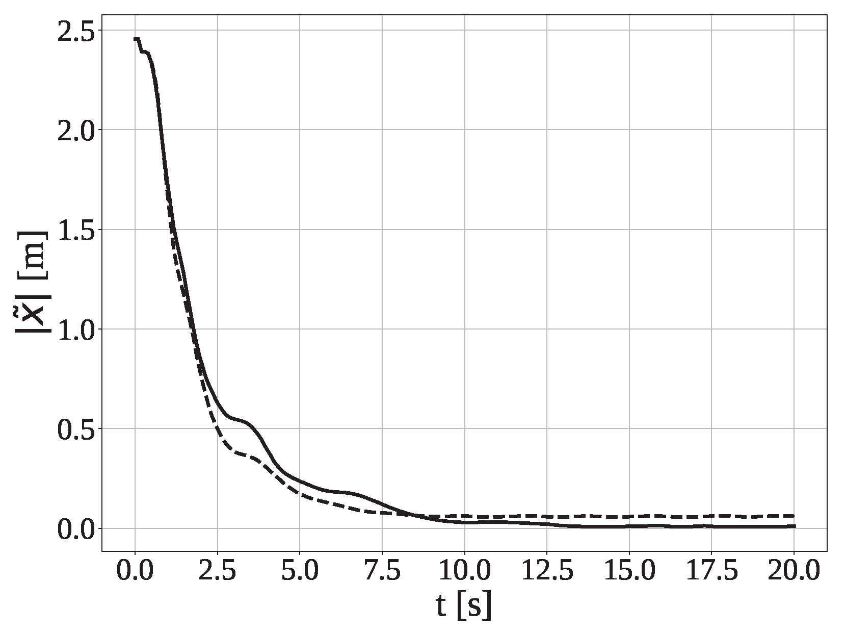
5.3. Comparison with Sliding-Mode Control

During the final experiment, the proposed controller was compared with SMC, which is a control technique that is well known for its robustness to external disturbances and parametric uncertainty; in this context, it represents a challenging benchmark for our control proposal. The SMC used is expressed as

$$\mathbf{u}={\mathbf{B}}_2^{-1}\mathbf{K}{\left[\mathrm{sign}{\left(\mathbf{s}\right)}^T-{\dot{\mathbf{x}}}^T\right]}^T,$$

(43)

where $\mathbf{K}$ has the same values as those in Table 1 in order to have a fair comparison, and $\mathbf{s}=\mathrm{diag}(2,2,10,20,20,20)\tilde{\mathbf{x}}-\dot{\mathbf{x}}$ is the sliding surface. Notice that the difference between (29) and (43) is that the first one compensates for the disturbances by means of their accurate estimation, whereas the latter uses the sliding-mode motion instead. The UAV is commanded to move to the target set point $(x_b^d,y_b^d,z_b^d)=(0,0,2)$ m with 10 degrees of orientation about $z_b$ for 20 s.

Figure 11 shows the norms of the error using both controllers. Even though both controllers provided a stable behavior of the norm of the error, a steady-state error of 5 cm could be appreciated with the SMC.

6. Conclusions

A robust control scheme for full-pose regulation and tracking of a UAV with a passively tilted hexarotor was presented in this work. The main contribution is the implementation of a theoretically sustained ADRC approach with a robust SMESO on a passively tilted hexarotor by employing a highly realistic simulator. It is worth highlighting that such a technique has not been reported in the literature for passively tilted hexarotors. Furthermore, the analysis of the stability of both the designed controller and the observer was presented by using a consistent theory that does not rely on a priori knowledge of the bound of the total disturbance, as several ADRC schemes in the literature do. As mentioned above, a simulator with physics motors was used during the presented work, the behavior of which was almost identical to that of a real UAV. In order to prove the effectiveness of the control system proposal, several case studies were carried out. Achieving the target trajectory was successful, since all of the states reached the target value with errors close to zero. Additionally, the proposed controller was effective under a payload and the simulation of continuous time-varying and discontinuous wind disturbances thanks to the perfect reconstruction of the external disturbances, which was consistent with the theoretical hypothesis of the convergence of the observer regarding the non-differentiable total disturbance. The proposed controller yielded a recovery time that was shorter than five seconds, reached the set point with a significantly low overshoot for the worst case, and remained within an acceptable range when under solid disturbances. The presented control approach performed better than the SMC because it yielded significantly less steady-state norm of the error for full-pose regulation. These successful results prove the effectiveness of the proposed control technique and provide motivation for its application to other UAVs.

References

1. Lee, S.J.; Kim, S.; Johansson, K.H.; Kim, H.J. Robust acceleration control of a hexarotor UAV with a disturbance observer. In Proceedings of the 2016 IEEE 55th Conference on Decision and Control (CDC), Las Vegas, NV, USA, 12–14 December 2016; pp. 4166–4171. [Google Scholar]
2. Dai, B.; He, Y.; Zhang, G.; Gu, F.; Yang, L.; Xu, W. Wind disturbance rejection for unmanned aerial vehicle based on acceleration feedback method. In Proceedings of the 2018 IEEE Conference on Decision and Control (CDC), Miami Beach, FL, USA, 17–19 December 2018; pp. 4680–4686. [Google Scholar]
3. Li, D.; Liu, H.H. Sensor bias fault detection and isolation in a large multirotor aerial vehicle using active disturbance rejection control. In 2018 AIAA Information Systems-AIAA Infotech@ Aerospace; AIAA: Reston, VA, USA, 2018; p. 0249. [Google Scholar]
4. Ding, L.; Zhou, J.; Shan, W. A hybrid high-performance trajectory tracking controller for unmanned hexrotor with disturbance rejection. Trans. Can. Soc. Mech. Eng. 2018, 42, 239–251. [Google Scholar] [CrossRef]
5. Arellano-Quintana, V.M.; Portilla-Flores, E.A.; Merchán-Cruz, E.A. Multi-objective design optimization of a hexa-rotor with disturbance rejection capability using an evolutionary algorithm. IEEE Access 2018, 6, 69064–69074. [Google Scholar] [CrossRef]
6. Chen, Z.; Stol, K.; Richards, P. Preliminary design of multirotor UAVs with tilted-rotors for improved disturbance rejection capability. Aerosp. Sci. Technol. 2019, 92, 635–643. [Google Scholar] [CrossRef]
7. Xu, H.; Yang, Z.; Lu, K.; Xu, C.; Zhang, Q. Control of a Tilting Hexacopter under Wind Disturbance. Math. Probl. Eng. 2020, 2020, 9465153. [Google Scholar] [CrossRef]
8. Kotarski, D.; Piljek, P.; Brezak, H.; Kasać, J. Chattering-free tracking control of a fully actuated multirotor with passively tilted rotors. Trans. FAMENA 2018, 42, 1–14. [Google Scholar] [CrossRef]
9. Yao, C.; Krieglstein, J.; Janschek, K. Modeling and Sliding Mode Control of a Fully-actuated Multirotor with Tilted Propellers. IFAC-PapersOnLine 2018, 51, 115–120. [Google Scholar] [CrossRef]
10. Arizaga, J.M.; Castañeda, H.; Castillo, P. Adaptive Control for a Tilted-Motors Hexacopter UAS Flying on a Perturbed Environment. In Proceedings of the 2019 International Conference on Unmanned Aircraft Systems (ICUAS), Atlanta, GA, USA, 11–14 June 2019; pp. 171–177. [Google Scholar]
11. Nguyen, N.P.; Kim, W.; Moon, J. Super-twisting observer-based sliding mode control with fuzzy variable gains and its applications to fully-actuated hexarotors. J. Frankl. Inst. 2019, 356, 4270–4303. [Google Scholar] [CrossRef]
12. Kase, S.; Oya, M. Adaptive tracking controller for hexacopters with a wind disturbance. Artif. Life Robot. 2020, 25, 322–327. [Google Scholar] [CrossRef]
13. Rashad, R.; Kuipers, P.; Engelen, J.; Stramigioli, S. Design, modeling, and geometric control on SE (3) of a fully-actuated hexarotor for aerial interaction. arXiv 2017, arXiv:1709.05398. [Google Scholar]
14. Rashad, R.; Califano, F.; Stramigioli, S. Port-Hamiltonian passivity-based control on SE (3) of a fully actuated UAV for aerial physical interaction near-hovering. IEEE Robot. Autom. Lett. 2019, 4, 4378–4385. [Google Scholar] [CrossRef]
15. Ryll, M.; Muscio, G.; Pierri, F.; Cataldi, E.; Antonelli, G.; Caccavale, F.; Bicego, D.; Franchi, A. 6D interaction control with aerial robots: The flying end-effector paradigm. Int. J. Robot. Res. 2019, 38, 1045–1062. [Google Scholar] [CrossRef] [Green Version]
16. Huang, Y.; Xue, W. Active disturbance rejection control: Methodology and theoretical analysis. ISA Trans. 2014, 53, 963–976. [Google Scholar] [CrossRef] [PubMed]
17. Roy, S.; Baldi, S.; Li, P.; Sankaranarayanan, V.N. Artificial-delay adaptive control for underactuated Euler–Lagrange robotics. IEEE/ASME Trans. Mechatron. 2021, 26, 3064–3075. [Google Scholar]
18. Sankaranarayanan, V.N.; Roy, S.; Baldi, S. Aerial transportation of unknown payloads: Adaptive path tracking for quadrotors. In Proceedings of the 2020 IEEE/RSJ International Conference on Intelligent Robots and Systems (IROS), Las Vegas, NV, USA, 24 October–24 January 2020; pp. 7710–7715. [Google Scholar]
19. Guo, B.Z.; Zhao, Z.L. On convergence of non-linear extended state observer for multi-input multi-output systems with uncertainty. IET Control Theory Appl. 2012, 6, 2375–2386. [Google Scholar] [CrossRef]
20. Sira-Ramírez, H.; Luviano-Juárez, A.; Ramírez-Neria, M.; Zurita-Bustamante, E.W. Active Disturbance Rejection Control of Dynamic Systems: A Flatness Based Approach; Butterworth-Heinemann: Oxford, UK, 2018. [Google Scholar]
21. Guo, B.Z.; Zhao, Z.L. Active Disturbance Rejection Control for Nonlinear Systems: An Introduction; John Wiley & Sons: Hoboken, NJ, USA, 2016. [Google Scholar]
22. Orozco-Soto, S.M.; Ibarra-Zannatha, J.M. Motion control of humanoid robots using sliding mode observer-based active disturbance rejection control. In Proceedings of the 2017 IEEE 3rd Colombian Conference on Automatic Control (CCAC), Cartagena, Colombia, 8–20 October 2017; pp. 1–8. [Google Scholar]
23. Spurgeon, S.K. Sliding mode observers: A survey. Int. J. Syst. Sci. 2008, 39, 751–764. [Google Scholar] [CrossRef]
24. Drakunov, S.; Utkin, V. Sliding mode observers. Tutorial. In Proceedings of the 1995 34th IEEE Conference on Decision and Control, New Orleans, LA, USA, 13–15 December 1995; Volume 4, pp. 3376–3378. [Google Scholar]
25. Patel, R.V.; Toda, M.; Sridhar, B. Robustness of linear quadratic state feedback designs in the presence of system uncertainty. IEEE Trans. Autom. Control 1977, 22, 945–949. [Google Scholar] [CrossRef]
26. Khalil, H.K. Nonlinear Systems; Prentice Hall: Hoboken, NJ, USA, 2002. [Google Scholar]
27. Michieletto, G.; Ryll, M.; Franchi, A. Fundamental actuation properties of multirotors: Force–moment decoupling and fail–safe robustness. IEEE Trans. Robot. 2018, 34, 702–715. [Google Scholar] [CrossRef]
28. Ruggiero, F.; Cacace, J.; Sadeghian, H.; Lippiello, V. Passivity-based control of VToL UAVs with a momentum-based estimator of external wrench and unmodeled dynamics. Robot. Auton. Syst. 2015, 72, 139–151. [Google Scholar] [CrossRef]
29. Poznyak, A.; Polyakov, A.; Azhmyakov, V. Attractive Ellipsoids in Robust Control; Springer: Berlin, Germany, 2014. [Google Scholar]
30. Ryll, M.; Bicego, D.; Franchi, A. Modeling and control of FAST-Hex: A fully-actuated by synchronized-tilting hexarotor. In Proceedings of the 2016 IEEE/RSJ International Conference on Intelligent Robots and Systems (IROS), Daejeon, Korea, 9–14 October 2016; pp. 1689–1694. [Google Scholar]
31. Siciliano, B.; Sciavicco, L.; Villani, L.; Oriolo, G. Robotics: Modelling, Planning and Control; Springer Science & Business Media: Berlin, Germany, 2010. [Google Scholar]
32. Rajappa, S.; Ryll, M.; Bülthoff, H.H.; Franchi, A. Modeling, control and design optimization for a fully-actuated hexarotor aerial vehicle with tilted propellers. In Proceedings of the 2015 IEEE international conference on robotics and automation (ICRA), Seattle, WA, USA, 25–30 May 2015; pp. 4006–4013. [Google Scholar]
33. Joseph, L.; Cacace, J. Mastering ROS for Robotics Programming—Second Edition: Design, Build, and Simulate Complex Robots Using the Robot Operating System, 2nd ed.; Packt Publishing: Birmingham, UK, 2018. [Google Scholar]
34. Furrer, F.; Burri, M.; Achtelik, M.; Siegwart, R. RotorS—A Modular Gazebo MAV Simulator Framework; Springer: Berlin, Germany, 2016; Chapter Robot Operating System (ROS); Volume 625, pp. 595–625. [Google Scholar]
Figure 1. Hexarotor with tilted propellers and reference frames. O W is the world reference frame and O B is the airframe coordinate frame. O S i is the coordinate frame of the i-th propeller.
Drones 06 00258 g001
Figure 2. Left: Top view of the tilted hexarotor indicating each rotor’s spin direction, ω i , and the length L from the CoM of the airframe to the center of rotation of a rotor; in this case, ζ i = π / 3 . All of the rotors are equidistant with respect to the CoM, and the location angle of each rotor with respect to the last one is the same. Right: Front view of the hexarotor with two examples of the tilting angles α . All six of the rotors are tilted with the same magnitude, but in different senses.
Drones 06 00258 g002
Figure 3. Block diagram of the proposed controller and observer. Everything within the dashed line is component-wise for i = 1 , 2 , , 6 .
Drones 06 00258 g003
Figure 4. Time evolution of the norm of the state error while the UAV performed the commanded Cartesian trajectory.
Drones 06 00258 g004
Figure 5. Cartesian motion of the UAV. Desired trajectory. – – UAV’s trajectory.
Drones 06 00258 g005
Figure 6. Top: Behaviors of the states of the UAV during a regulation task when subjected to sudden gusts of wind. Set points. —- Measured states. Observed states. Bottom: Reconstructed total disturbances about each axis. All of the horizontal axes display the time in seconds.
Drones 06 00258 g006
Figure 7. Top: Behaviors of the states of the UAV during a regulation task when subjected to wind blows. Set points. —- Measured states. Observed states. Bottom: Reconstructed total disturbances about each axis. All of the horizontal axes display the time in seconds.
Drones 06 00258 g007
Figure 8. Time evolution of the rotors’ velocities. Left: Experiment on regulation under wind shear. Right: Experiment on regulation under smooth blowing of wind. ω 1 , ω 2 , ω 3 , ω 4 , ω 5 , ω 6 .
Drones 06 00258 g008
Figure 9. Left: Time evolution of the norms of the state error. Right: Time evolution of the estimated disturbance along the z B axis, which was retrieved from the SMESO.
Drones 06 00258 g009
Figure 10. Time evolution of the rotors’ velocities for the experiment on regulation under payload conditions. ω 1 , ω 2 , ω 3 , ω 4 , ω 5 , ω 6 .
Drones 06 00258 g010
Figure 11. Time evolution of the norms of the state error while the UAV performed a regulation task. —- ADRC. SMC.
Drones 06 00258 g011