Article

Model Predictive Control Technique for Ducted Fan Aerial Vehicles Using Physics-Informed Machine Learning

1
Key Laboratory of Autonomous Systems and Networked Control, Ministry of Education, Unmanned Aerial Vehicle Systems Engineering Technology Research Center of Guangdong, School of Automation Science and Engineering, South China University of Technology, Guangzhou 510640, China
2
School of Automation, Beijing Institute of Technology, Beijing 100081, China
*
Author to whom correspondence should be addressed.
Submission received: 28 November 2022 / Revised: 18 December 2022 / Accepted: 20 December 2022 / Published: 21 December 2022

Abstract

:
This paper proposes a model predictive control (MPC) approach for ducted fan aerial robots using physics-informed machine learning (ML), where the task is to fully exploit the capabilities of the predictive control design with an accurate dynamic model by means of a hybrid modeling technique. For this purpose, an indigenously developed ducted fan miniature aerial vehicle with adequate flying capabilities is used. The physics-informed dynamical model is derived offline by considering the forces and moments acting on the platform. On the basis of the physics-informed model, a data-driven ML approach called adaptive sparse identification of nonlinear dynamics is utilized for model identification, estimation, and correction online. Thereafter, an MPC-based optimization problem is computed by updating the physics-informed states with the physics-informed ML model at each step, yielding an effective control performance. Closed-loop stability and recursive feasibility are ensured under sufficient conditions. Finally, a simulation study is conducted to concisely corroborate the efficacy of the presented framework.

1. Introduction

1.1. Literature Review

The ducted fan aerial vehicles (DFAVs) are a type of vertical take-off and landing platforms that have the innate capabilities of a helicopter and fixed-wing aircraft [1,2]. These airborne vehicles are used in a wide number of applications in different areas such as transportation, inspection, aerial surveillance, and manipulation [3,4]. Due to their annular fuselage mechanism called duct [5], these aerial robots are known for their safety in congested, cluttered, and hazardous environments [6,7]. Having vector thrust capabilities [8], DFAVs also have several advantages over other configurations, such as fixed-wing platforms, helicopters, open-rotor, and shrouded quadrotors [9]. However, complex flow distribution makes it arduous to model these aircraft accurately [10], consequently making the flight control design more challenging.
Over the years, several flight control systems based on different strategies have been presented to control these vehicles [9]. In this regard, model predictive control (MPC) has proved itself as an advanced control approach that can address many issues associated with aerial applications [11]. One of the simplest techniques is linear MPC, which has been employed for the purpose of attitude control for these aerial platforms [12,13]. An improved unified control framework based on linear MPC for position and attitude control with Kalman filter as a disturbance observer (DOB) has also been studied and validated [14]. Moreover, robust MPC with a DOB and adaptive MPC with two DOBs have been presented to compensate for the effect of model inaccuracies and disturbances [15]. For achieving similar tasks with some improvements compared to robust MPC [15], composite disturbance rejection approaches based on MPC, referred to as MPC-based compound flight control (MPC-CFC), have been proposed [16,17].
In the aforementioned works, some problems can be solved to improve the control performance of future MPC-driven control systems.
  • The performance of MPC depends on the accurate model of the system dynamics [18,19], which is challenging to obtain. This problem is even more prevalent in flight control, where varying flight conditions, disturbances, faults, and model uncertainties may lead to ineffective control performance.
  • In the disturbance rejection MPC framework based on DOB (e.g., [16,17]), the dynamics of the disturbance profile cannot be faster than the dynamics of DOB, which implies that this type of composite method is not suitable to estimate and compensate for fast time-varying disturbances.
There are two types of dominant techniques for dynamical system modeling [20]: (1) Physics-informed dynamics, where the equations of motion are derived from governing physical rules, and (2) machine learning (ML) based data-driven system modeling [21]. To construct an end-to-end dynamical model, these techniques are employed separately. There is a growing potential for integrating data-driven techniques based on ML in the aerospace industry [22]. One of the commonly used ML techniques is the neural network (NN) [23,24,25,26]. Nevertheless, NN-based methods need massive training data, which may be uninterpretable and difficult to include constraints. These reasons limit their utilization for online system identification [27]. One alternative is to use sparse identification of nonlinear dynamics (SINDy) developed in [28], which has shown effective control and predictive capabilities with MPC in the presence of noise and is more suitable for low and medium data than the NN technique. Moreover, it has demonstrated strong parametric robustness, effective training, and execution time [27]. While the SINDy algorithm is an effective strategy for multiple learning, an adaptive SINDy technique is more suitable that can efficiently update and correct the dynamics online in a repetitive fashion [29,30]. However, it is challenging to seamlessly capture the correct model with ML techniques alone to satisfy the conservation laws and constraints. On the other hand, physics-informed dynamical models can capture constraints and conservation laws. However, they are either too simple or ultra-complex that may become too expensive to handle online due to high computational costs, particularly for varying system dynamics for MPC. In this aspect, a physics-informed ML hybrid-modeling technique can be employed to seamlessly incorporate physical models and data in all circumstances involving high-dimensional, physically understood, and uncertain contexts [31,32,33,34,35,36].

1.2. Contributions

Motivated by the above discussion, this article presents an MPC-based control strategy for DFAVs via a hybrid modeling approach called physics-informed ML. First, the physics-informed model (nominal system) for the aerial robot is constructed by considering the forces and moments offline. Moreover, it is considered that the nominal system is not affected by any disturbances or uncertainties. Thereafter, a data-driven approach called adaptive SINDy is employed for estimating and compensating for any parametric changes online during the flight. The optimization problem is solved online, where in each step, the physics-informed system is updated by the physics-informed ML. This way, the control action applied to the aerial vehicle is optimal with respect to the current state. In Table 1, the advantages and disadvantages of existing techniques over the proposed scheme are provided. The contributions of this manuscript are expressed in the following manner:
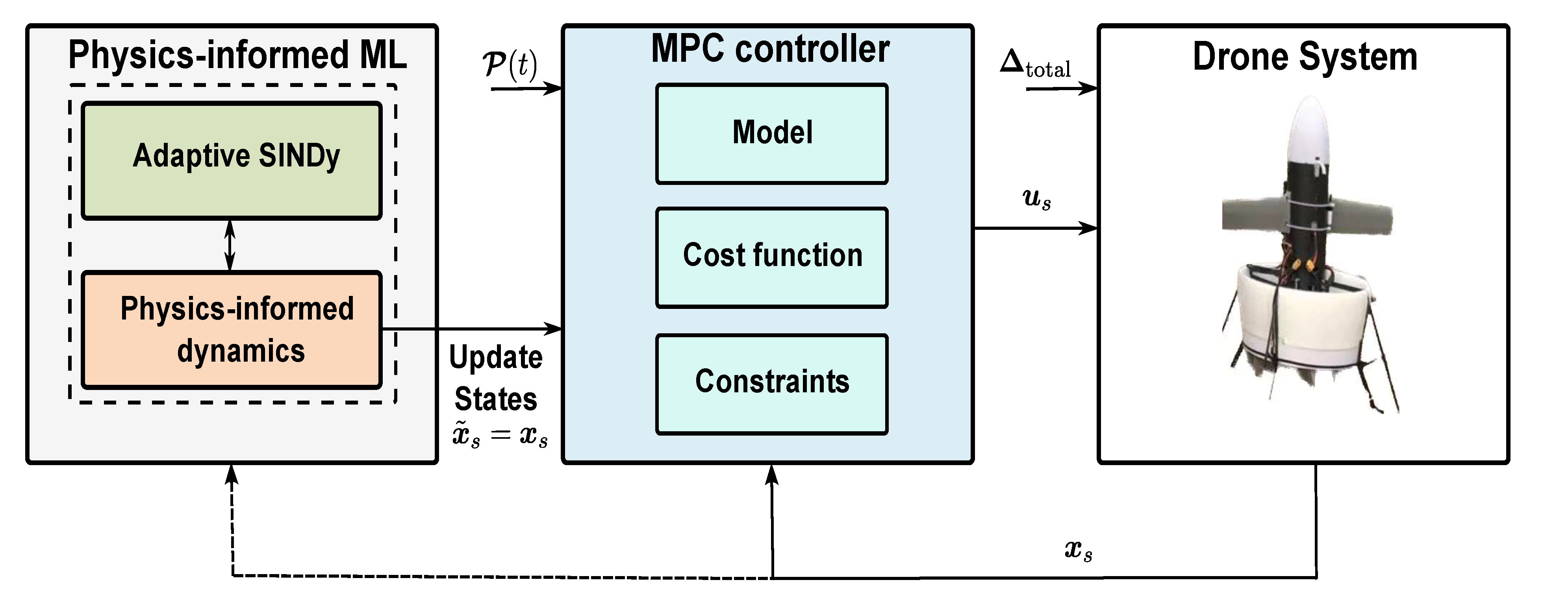
  • To fully exploit the potential of MPC, an online-based predictive control algorithm using physics-informed ML without the utilization of DOB is presented, unlike [15,16,17]. By employing the methodology in such a way, the inherent issues encountered in the disturbance rejection MPC framework [16,17] can be solved.
  • For efficient response and to avoid any usual computational complexity problem, only the data-driven part in the hybrid modeling is determined online for model correction. To further enhance the computational efficiency of the developed control algorithm, the physics-informed model is also updated by the physics-informed ML model in each step while solving the optimization problem.
  • Unlike [12,13,14,15], theoretical properties such as recursive feasibility and closed-loop stability with constraints satisfaction under sufficient conditions are derived.
  • In contrast to the existing disturbance rejection framework [16], the designed approach demonstrates effective performance. Furthermore, the constructed approach can be implemented in other robotics systems to attain similar goals.

1.3. Organization

In Section 2, the problem formulation is constructed in the physics-informed modeling and physics-informed ML model subsections. Furthermore, control objectives are defined, and a few assumptions with preliminaries are established for smooth control operation. The control approach includes MPC development and its feasibility and stability proofs and is provided in Section 3. Section 4 illustrates the numerical implementation that includes comparative analysis with some discussion. Section 5 concludes the article.

1.4. Notation

N and R denote all non-negative integers and real space, respectively. ( . ) ( . ) T ( . ) is the Euclidean norm. diag { ( . ) 11 , ( . ) 22 , . . . , ( . ) n } denotes the diagonal matrix with entries ( . ) 11 , , ( . ) n R . Q-weighted norm is referred to as ( . ) Q ( . ) T Q ( . ) , where Q denotes a positive definite matrix. Consider any given system state/input as ∘, τ | t l means ∘ at τ predicted at t l . Superscript * is utilized to define state/input after optimization. Accents ˜ and ^ represent the nominal state/nominal control input and estimated state/input, respectively. In the entire manuscript, physics-informed dynamics and physics-informed ML are referred to as nominal and real systems, and these terms are used interchangeably. A bold font style is employed to represent vectors and matrices.

2. Problem Formulation

The hybrid modeling procedure is divided into two phases, i.e., physics-informed modeling (offline) and data-driven scheme (online), which is based on lots of physics and less data, shown in Figure 1.

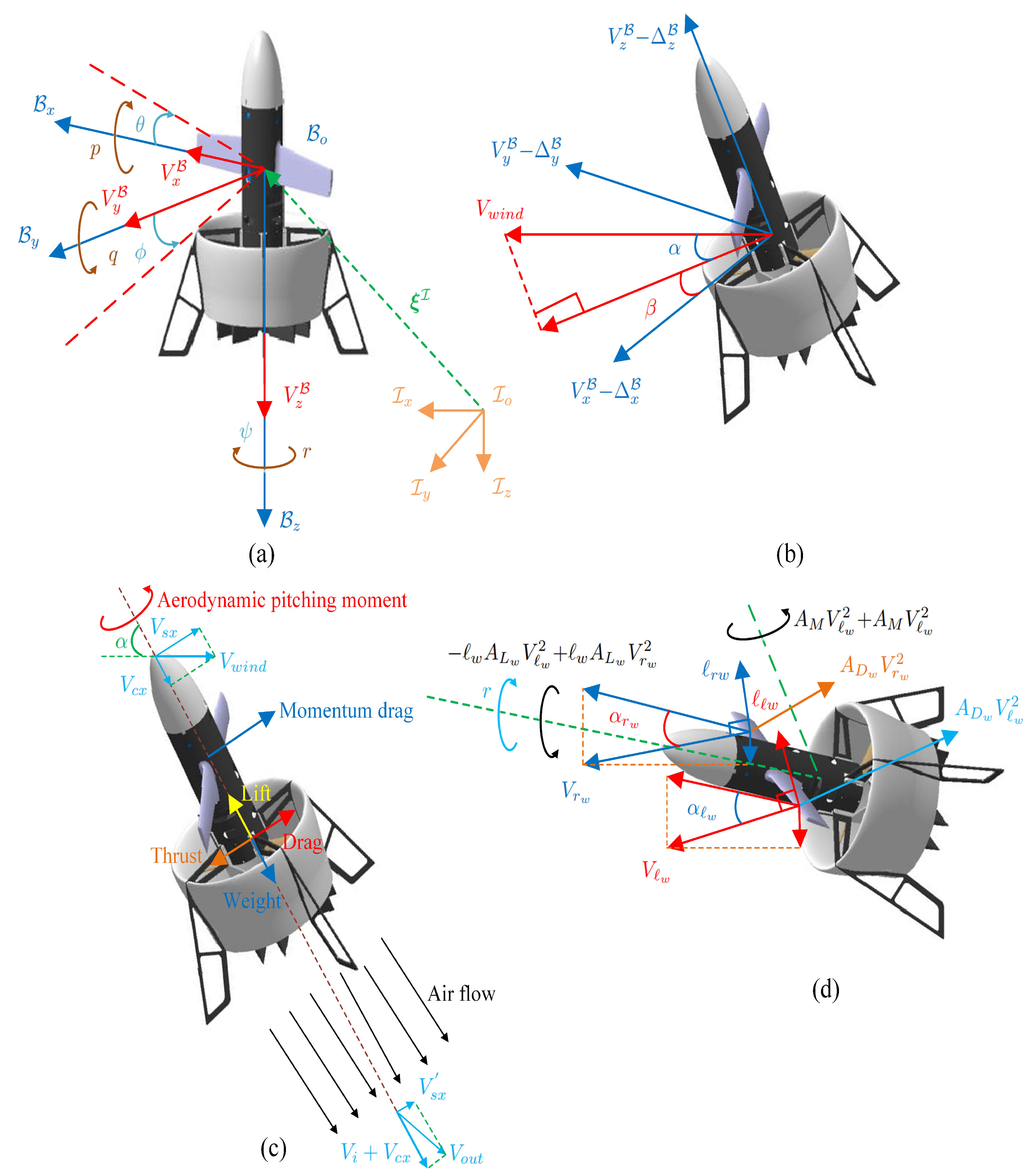
2.1. Physics-Informed Modelling

In Figure 2, the ducted fan aerial robot is represented by two coordinate frames, i.e., body-fixed frame B f { B o , B x , B y , B z } and inertial frame I f { I o , I x , I y , I z } . ξ I = [ ξ x I , ξ y I , ξ z I ] T R 3 , V I = [ V x I , V y I , V z I ] T R 3 , V B = [ V x B , V y B , V z B ] T R 3 and ω B = [ p , q , r ] T R 3 are position, linear velocity in I f , linear velocity in B f , and angular velocity, respectively. Δ w i n d = Δ x B ( t ) , Δ y B ( t ) , Δ z B ( t ) T are disturbances acting on the flying robot. Θ = [ ϕ , θ , ψ ] T R 3 denotes the attitude of the aircraft, where ϕ , θ and ψ are roll, pitch, and yaw angle, respectively. From these rotation angles, the rotational matrix T B I S O ( 3 ) from B f and I f can be defined as (see among others, e.g., [9]):
T B I = C ψ C θ C ψ S θ S ϕ S ψ C ϕ C ψ S θ C ϕ + S ψ S ϕ S ψ C θ S ψ S θ S ϕ + C ψ C ϕ S ψ S θ C ϕ C ψ S ϕ S θ C θ S ϕ C θ C ϕ ,
where C ( * ) = cos ( * ) and S ( * ) = sin ( * ) , with  ( * ) denotes any angle. The rotational kinematics of the airborne platform is described in the following form:
Θ ˙ = Ω ω B , Ω = C θ 0 S θ S θ S ϕ / C ϕ 1 C θ S ϕ / C ϕ S θ / C ϕ 0 C ϕ C ϕ .
Other flight components in Figure 2 are expressed as follows:
V w i n d = V x B Δ x B 2 + V y B Δ y B 2 + V z B Δ z B 2 , α = arccos V z B Δ z B V w i n d , 0 α π , β = arctan V y B Δ y B V x B Δ x B , π 2 β π 2 ,
where V w i n d , α , and β are denoted as airspeed, angle of attack, and side-slip angle, respectively. The translational and rotational dynamics of the VTOL aircraft can be formulated as
ξ ¨ I = V ˙ I = T B I F B / m + G a , ω ˙ B = I 1 M B + I ω B × ω B ,
where m, F B , M B , and I are the mass, total force, total moments, and diagonal matrix consisting of the moment of inertia, respectively. Moreover, G a = [ 0 0 g ] T , and g is the gravitational acceleration. Velocity of the airflow exhausted from the fan ( V a f ) can be expressed as:
V a f = V z B Δ z B 2 + V z B Δ z B 2 2 + T 2 ρ A f d ,
where T = A ω T ω r 2 is the thrust, and  ω r and A ω T denote the rotation speed and thrust coefficient, respectively. Moreover, ρ and A f d are the free air density and fan disk area, respectively. Next, we describe the local airspeed on left-wing ( V w ) and right-wing ( V r w ) with local α on left-wing ( α w ) and right-wing ( α r w ) are given as follows:
V w = V x B + r w Δ x 2 + V z B Δ z 2 , V r w = V x B r w Δ x 2 + V z B Δ z 2 , α w = C α l w = V z B Δ z / V w , 0 α w π , α r w = C α r w = V z B Δ z / V r w , 0 α r w π ,
where w represents the lever arm from the B z axis to the aerodynamic center of the left and right/left wing. Generally, an aircraft is affected by four main forces during flight (lift, weight, thrust, and drag), depicted in Figure 2c. In the current scenario, the  F B can be defined as follows:
F B = 0 0 A ω T ω r 2 Thrust   force + V w i n d 2 A L d C α + A D d S α C β A L d C α + A D d S α S β A L d S α + A D d C α Duct - body   force + A L w V w 2 C α w + A L w V r w 2 C α r w + A D w V w 2 S α w + A D w V r w 2 S α r w 0 A L w V w 2 S α w A L w V r w 2 S α r w + A D w V w 2 C α w + A D w V r w 2 C α r w Wing   force + ρ A f d V a f ζ r a t i o V x B Δ x B V y B Δ y B 0 Momentum   drag ,
where A L d and A D d are the lift and drag coefficients, respectively. Moreover, A D w and A L w represent the drag and lift coefficients of the half-wing section of the aircraft, respectively. ζ r a t i o denotes the damping ratio and is defined as
ζ r a t i o = V s x V s x V s x .
The total moment is expressed in the following manner:
M B = A c s V a f 2 l 1 δ 1 + l 1 δ 3 l 1 δ 2 + l 1 δ 4 l 2 δ 1 + l 2 δ 2 + l 2 δ 3 + l 2 δ 4 Control   surfaces + 0 0 k ω s ω r 2 Fan   torque + I f ω r q p 0 Gyroscopic   effect + ϵ d r a g ρ A f d V a f ζ r a t i o V x B Δ x B V y B Δ y B 0 + ϵ D V w i n d 2 A L d C α + A D d S α C β A L d C α + A D d S α S β A L d S α + A D d C α Aerodynamic   pitching   moment + 0 A M V w 2 + A M V w 2 w A L w V w 2 + w A L w V r w 2 Wing   moment + A a r V a f 2 Anti - rotation torque ,
where k ω s , ϵ d r a g , ϵ D , I f , A a r , l 1 , l 2 , A c s , δ i , and A M represent the rotation speed with respect to fan torque coefficient, lever arms of momentum drag, duct body force, fan inertia, constant coefficient, lever arms related to roll/pitch-axis, and yaw-axis, deflection angle to force coefficient, the deflection angle of i-th control surface, and moment coefficient of the half-wing section of the vehicle, respectively. Consider the drone’s system defined as follows:
x ˙ s = f s x s ( t ) , u s ( t ) ; η s , x s ( 0 ) = x 0 ,
where x s = [ ξ I V I Θ ω B ] T R 12 denotes the system states. f s and η s are the dynamics and the aircraft’s parameters. It is considered that the system (10) is directly affected by disturbances and uncertainties. u s ( t ) = [ T u s 2 T ] T R 4 represents control input, where u s 2 denotes the regulated moment input and is provided as follows:
u s 2 = u 11 u 12 u 13 = l 1 δ 1 + l 1 δ 3 l 1 δ 2 + l 1 δ 4 l 2 δ 1 + l 2 δ 2 + l 2 δ 3 + l 2 δ 4 .
Next, by considering only the physics-informed model of the aircraft as a nominal system:
x ˜ ˙ s ( t ) = f s x ˜ s ( t ) , u ˜ s ( t ) .
The discrepancy modeling problem is derived from the difference between the quantity of interest (i.e., forces and moments) from a physics-informed model ν m ( t ) and estimated value ν o ( t ) . Hence, discrepancy Δ ν ( t ) is expressed as:
Δ ν ( t ) = ν o ( t ) ν m ( t ) .
Under ideal conditions, the estimated value and physics-informed model may have the same magnitude in (12), i.e.,  Δ ν ( t ) 0 . Nonetheless, such an outcome in actual flight may not be possible due to several factors.

2.2. Data-Driven ML-Adaptive SINDy

Inspired by the existing work on learning from discrepancy model [20] and integrating it with adaptive SINDy by [30] for compensating for any abrupt changes in the system dynamics during different flight conditions of the DFAV, a hybrid modeling approach based on physics-informed dynamics and adaptive SINDy is constructed, shown in Figure 3. The sudden changes in the adaptive SINDy involve only addition, deletion, and modifications. This is useful as it enables us to effectively determine the new and missing terms with less data than to identify the entire model from scratch. There are three basic kinds of model changes in the adaptive SINDy:
  • Modification: If the whole model is unchanged except for model parameters, then least square regression will be employed on the known model to find new parameters;
  • Deletion: If a few terms are removed, then sparse regression can be utilized on the sparse coefficients to identify which terms have been taken out;
  • Addition: To find the model error, the SINDy regression will identify the sparsest combination of inactive terms.

2.2.1. Baseline Model

By using the standard procedure of SINDy, we measure the required number of snapshots m s of x s and u s and rearrange them into two data matrices X s and U s :
X s = ξ x I t 1 ξ y I t 1 ψ t 1 ξ x I t i ξ y I t i ψ t i ξ x I t m ξ y I t m ψ t m , U s = T t 1 u 11 t 1 u 13 t 1 T t i u 11 t i u 13 t i T t m u 11 t m u 13 t m ,
where t i is the sampling time. Simplify Equation (13) and transform it into the following form:
X s = x s 1 ( t 1 ) x s 2 ( t 2 ) x s 3 ( t 3 ) . . . x m s ( t m ) T , U s = u s 1 ( t 1 ) u s 2 ( t 2 ) u s 3 ( t 3 ) . . . u m s ( t m ) T ,
where u m s and x m s are control and state vector at the mth sampling time. The value of the aircraft’s state is calculated by the numerical differentiation.
X ˙ s = x ˙ s 1 ( t 1 ) x ˙ s 2 ( t 2 ) x ˙ s 3 ( t 3 ) . . . x ˙ m s ( t m ) T , = ξ ˙ x I t 1 ξ ˙ y I t 1 ψ ˙ t 1 ξ ˙ x I t i ξ ˙ y I t i ψ ˙ t i ξ ˙ x I t m ξ ˙ y I t m ψ ˙ t m .
The vehicle model depends primarily on the physics-informed modeling method with less concentration on the ML technique as it is mainly useful for any discrepancy and abrupt changes in the parametric values. Therefore, a similar assumption to [29] is required, i.e., either the obtained data are prefiltered through relevant frameworks [37,38] or it contains no noise interference. Next, a candidate library function Ξ ( X s , U s ) is developed using the data matrices X s and U s , in which selected function is arbitrary, and is either a trigonometric or polynomial function. In general, polynomial functions are a relatively basic choice. Therefore, the complexity of the library can be increased by including trigonometric functions. Nevertheless, both functions and physics-informed knowledge of the vehicle will be utilized to construct the library function:
Ξ ( X s , U s ) = 1 T , X s T , ( X s X s ) T , ( X s U s ) T , , S X s T , S U s T , ,
where X s X s and X s U s are defined as:
X s X s = ξ x I ξ x I t 1 ξ x I ξ y I t 1 ξ y I ξ y I t 1 ψ 2 t 1 ξ x I ξ x I t 2 ξ x I ξ y I t 2 ξ y I ξ y I t 2 ψ 2 t 2 ξ x I ξ x I t m ξ x I ξ y I t m ξ y I ξ y I t m ψ 2 t m , X s U s = ξ x I T t 1 ξ x I u 11 t 1 ξ y I u 11 t 1 ψ u 13 t 1 ξ x I T t 2 ξ x I u 11 t 2 ξ y I u 11 t 2 ψ u 13 t 2 ξ x I T t m ξ x I u 11 t m ξ y I u 11 t m ψ u 13 t m .
The dynamics of the vehicle model only depend on the few nonlinear terms in practice. The sparse model of f k ( . ) in system (10) can be set as follows:
f k ( X s , U s , χ k ) = j = 0 p s χ k j Λ j ( x s , u s ) , k = 1 , 2 , 3 , , 12 ,
where p s + 1 represents the number of candidate functions. χ k j and Λ j are the candidate functions of the j-th column in Ξ ( X s , U s ) and the weighted coefficient of Λ j ( x s , u s ) related to the k-th state, i.e.,  χ k = [ χ k 0 , χ k 1 , χ k 2 , , χ k p s ] T , respectively. In the third step, sparse optimization is employed to determine a sparse model:
χ k = arg min χ k X ˙ k s χ k Ξ ( X s , U s ) T 2 + λ k χ k 1 ,
where X ˙ k s and λ k denote the k-th row of X ˙ and sparsity-promoting hyper-parameter, respectively. The theoretical results for convergences of SINDy framework have been provided in [39]. The computed value of χ k is stored in sparse matrix Ψ :
Ψ = χ 01 χ 02 χ 0 k χ 0 n χ 11 χ 12 χ 1 k χ 1 n χ p 1 χ p 2 χ p k χ p n = χ 1 χ 2 χ k χ 12 .
The baseline model of the DFAV’s dynamics can be written in the following expression:
X s Ξ ( X s , U s ) Ψ .
To summarize the entire process, the baseline model is determined, and a grid search is employed to identify the optimal hyper-parameter selection. In grid-search, all the combinations of hyper-parameters are evaluated, and the best available set is chosen. This process is executed one time to find the best set of hyper-parameters for future updates. The baseline model can be expressed as sparse coefficients in χ 0 .

2.2.2. Estimation of Model Divergence

Due to various factors (e.g., flight condition, nonlinearity, turbulence, actuator faults, etc.), the model parameters may vary at different times, resulting in divergence problems. Hence, a prediction framework that can quickly estimate any variation in the vehicle model is needed. In this work, the classical-predictor–correction approach is utilized to detect the variation caused by the aforementioned factors [40]. The predictor step is executed over a time τ ¯ during the interval t , t + τ ¯ using a valid model at time t. The divergence of the predictor x ^ s and measured state x s is calculated at t + τ as x d i v = x ^ s ( t + τ ) x s ( t + τ ) . The main theme is to determine when the model and the related state measurements diverge faster as opposed to the predicted ones by the dynamics of the system. Among many techniques, the divergence of the trajectory can be expressed by the Lyapunov exponent:
λ = lim τ lim x d i v t 0 0 log x d i v t 0 + τ x d i v t 0 τ ,
and its inverse sets of fastest time scale [30]. Since the information about the dynamical system for the prediction step, the Lyapunov exponent is computed via tangent space. The requirement for an effective detection necessitates computing tolerance λ d i v and determining the divergence time. If the prediction horizon by the local Lyapunov exponent and provided time scale are inconsistent, a divergence issue will arise between the measurements and the model. In the start, when the predicted and measured values deviate, then the divergence horizon is defined as:
T d i v ( t ) = arg min t d i v x ^ s ( t + t d i v ) x s ( t + t d i v ) > λ d i v .
Hence, it is assumed that, at time t, the real system and prediction model diverge if the model value and measured time scale differ:
λ ¯ d i v ( t ) > log λ d i v log ( x d i v ( t ) ) T d i v ( t ) ,
where λ d i v is the maximum value obtained from (22) during the time scale [ t , t + T d i v ] , & λ ¯ d i v = λ d i v ( t ) t [ t , t + T d i v ] with λ d i v ( t ) = max ( λ d i v 1 , λ d i v 2 , λ d i v 3 , , λ d i v 12 ) .

2.2.3. Adaptive Model Recovery

The following process is implemented for the quick recovery of model parameters. In the beginning, new data onto the existing sparse data χ 0 are regressed to determine varying parameters. Thereafter, the deletion of terms is identified by executing the sparse regression on the columns of Ξ that in χ 0 corresponds to the nonzero rows. In the presence of a residual error, a sparse model in the inactive columns of Ξ that corresponds to zero rows in χ 0 is fit for this error. Through this process, new terms may be introduced. This procedure is only performed when there is a divergence issue present.

2.3. Control Objective

By considering the physics-informed model as a nominal system x ˜ s and real system x s obtained as a result of the physics-informed ML procedure, suppose the aerial vehicle is flying with speed υ , and the plane follows a reference trajectory x ref in the presence of different factors (e.g., disturbances, uncertainties, actuator faults). From a control perspective, the tracking error of both control input e u = u s u ref and aircraft’s state e x = x s x ref needs to be minimized. Similarly, e ˜ x and e ˜ u represent nominal state and control input tracking error, respectively. Hence, the cost function is designed as follows:
J e ˜ x ( t ) , e ˜ u ( t ) = t t + t p S c e ˜ x ( τ | t ) , e ˜ u ( τ | t ) d τ Stage   cos t + T p e ˜ x ( t + t p | t ) Terminal   penalty , J e ˜ x ( t ) , e ˜ u ( t ) = t t + t p e ˜ x ( τ | t ) Q 2 + e ˜ u ( τ | t ) P 2 d τ Stage   cost + e ˜ x ( t + t p | t ) R 2 Terminal   penalty ,
where t p = n s t i represents the prediction horizon with n s denoting the predictive step. Moreover, P , Q , and R are the positive definitive weighting matrices in (25).
For the smooth and effective functioning of controller design, some preliminaries are needed before proceeding to the main control framework. Recall the nominal system (11), where only physics-informed modeling is considered.
Assumption 1.
It is assumed that f s x ˜ s ( t ) , u ˜ s ( t ) is Lipschitz continuous with u ˜ s U MPC is locally Lipschitz with a constant L in x ˜ s ( t ) . Hence, the following condition f s x ˜ s 1 , u ˜ s f s x ˜ s 2 , u ˜ s L x ˜ s 1 x ˜ s 2 holds.
Assumption 2.
We assume that nominal system (11) is known and differentiable with all the initial states available. Thus, one can use Jacobian linearization at the origin, which is assumed to be stabilizable. With this assumption, a linear state feedback control law u s = K e ˜ x can be obtained in such a form that is asymptotically stable if no disturbances are present.
To further elaborate on the nature of the control system, Assumption A2 from [16] with an additional condition can be adopted in the following assumption:
Assumption 3.
(i) For the nominal tracking error, the terminal controller and terminal region T are such that, if e ˜ x t l + t p | t l T , then by applying u ˜ s τ | t l + 1 = K e ˜ x τ | t l + 1 to the vehicle over the time interval τ t l + t p , t l + 1 + t p , it satisfies the following expressions of the locally stabilizing controller:
e ˜ x τ | t l T , u ˜ s = K e ˜ x U MPC .
(ii) the condition related to stage and terminal cost is provided as follows:
T ˙ p e ˜ x τ | t l + S c e ˜ x τ | t l , e ˜ u τ | t l 0 .
Remark 1.
Assumption 3 in (26) is a standard assumption employed in the MPC community [41]. However, in the current scenario, its usage is only restricted to an ideal situation, and the linear state feedback control law in Assumption 2 is only available if the tracking error lies in the terminal region, which is not always the case in the control system for an aircraft.
Several techniques to determine the terminal region have been developed over the years (e.g., [42,43,44]). Inspired by [16], a terminal region is defined as:
T = e ˜ x : F ˜ 1 | e ˜ ξ | + F ˜ 2 | e ˜ V | + F ˜ 3 | e ˜ Θ | + F ˜ 4 | e ˜ ω | < 1 ϰ ,
where ϰ can be appropriately selected based on the control design. F ˜ and e ˜ ( ) are the feedback gains and state error between reference and actual trajectory with parameters satisfying p ι q ι 0.25 , F ˜ ι 1 ± 1 4 p ι q ι p ι q ι , ι { 1 , 2 , 3 , . . . , 12 } .
Furthermore, disturbances are also present in the system. Therefore, an assumption is needed to prove the recursive feasibility and stability in the subsequent section.
Assumption 4.
It is assumed that turbulence Δ ext may also be present along with Δ w i n d . Hence, the dynamics of total disturbances acting on the aircraft are defined as:
Δ ˙ total = Δ ext + Δ w i n d , = [ Δ v Δ ω ] T + Δ w i n d ,
where Δ v and Δ ω denote the turbulence acting on the translational and rotational components of the vehicle. It is assumed that the total disturbances are bounded, i.e.,  Δ total , which can be fast-time varying unlike [16].
Furthermore, crucial definitions related to stability proof are given as follows:
Definition 1.
[45] The tracking error system is input-to-state stable (ISS), if there exists a K L function Γ ( · , · ) : R 0 × R 0 R & K function Υ ( · ) such that t 0 , it satisfies that
e x ( t ) Γ e x t 0 , t + Υ ( ) .
Definition 2.
[45] A function V ( . ) is referred to as ISS-Lyapunov function for tracking error system, if there exist K functions i ( . ) , and  K function ( . ) such that e x R 2
1 e x t l V e x t l 2 e x t l ,
V e x t l + 1 V e x t l 3 e x t l + ( ) .
If the Definitions 1 and 2 satisfy and no disturbances are acting on the aerial vehicle, then the tracking error also vanishes [46].

3. Control Framework

This section explains the presented control approach, illustrated in Figure 4. Reference trajectory P is employed to generate a particular flight envelop in different scenarios during the time interval t [ 0 , 10 ] , which is expressed as:
P ( t ) = ξ ref , V ref , η ref , ω ref T .
The optimization control problem is solved at a time sequence t l | l N , t l + 1 t l = t i :
Problem 1.
min u ˜ s τ | t l J e ˜ x ( t ) , e ˜ u ( t ) ,
subject to x ˜ s t l | t l = x s t l ,
x ˜ ˙ s τ | t l = f s x ˜ s τ | t l , u ˜ s τ | t l ,
u ˜ s τ | t l U MPC ,
x ˜ s τ | t l X ,
e ˜ x τ | t l t p × ϖ τ t l ,
e ˜ x t l + t p | t l T ϑ ,
where T ϑ = e ˜ x : e ˜ x ϑ is a robust terminal region, and  ϖ is designed as follows:
ϖ = υ ϰ ( F 1 2 + F 2 2 + F 3 2 + F 4 2 ) 1 / 2 , ϑ < ϖ ,
Remark 2.
For Problem 1, the nominal system (physics-informed dynamics) is updated by the actual state (physics-informed ML model) at each step. Consequently, the provided optimization problem must be solved online. Nevertheless, such an updating framework produces an optimal state with respect to the current one, and since the disturbances are not considered in Problem 1, the designed optimization problem consumes less computational resources.
Problem 1 determines the minimizing sequence over the interval [ t l , t l + t p ) :
u ˜ s * t l = u ˜ s * t l | t l , u ˜ s * t l + 1 | t l , , u ˜ s * t l + N | t l .
Hence, the drone’s control signal over interval t l , t l + 1 is defined as:
u s = u ˜ s * t l | t l ,
where u ˜ s * t l | t l is the initial control action of u ˜ s * t l .
A systematic procedure to apply the control action to the aircraft is provided in Algorithm 1. Nonetheless, if we assume that unknown disturbances are present, a tracking error between the reference and actual trajectory may exist. Furthermore, in order to satisfy the state constraints in the presence of the disturbances, the error on the upper bound between the actual and predicted nominal state is given as follows:
x s t l + 1 x ˜ s * t l + 1 | t l = x s t l + t l t l + 1 f s x s ( τ ) , u ˜ s ( τ ) d τ x ˜ s * t l | t l t l t l + 1 f s x ˜ s * τ | t l , u ˜ s * t l | t l d τ , t i + υ t l t l + 1 x s ( τ ) x ˜ s * τ | t l d τ , t i e υ t i .
Algorithm 1: MPC-based control using physics-informed ML
Drones 07 00004 i001
Theorem 1.
Suppose the Assumptions 2 and 3 hold, and the Problem 1 is feasible at initial time t 0 . Then, Problem 1 is feasible for all intervals under Algorithm 1, if the following conditions satisfy:
e υ t p t i ( ϖ ϑ ) , F ˜ t i ln ( ϖ ) ln ( ϑ ) ,
where F ˜ = min F ˜ i .
ϑ ϖ ( t p t i ) t p .
Proof. 
A feasible control sequence u ˜ s τ | t l + 1 at t l + 1 is provided as follows:
u ˜ s τ | t l + 1 = u ˜ s * τ | t l , τ t l + 1 , t l + t p , K e ˜ x τ | t l , τ t l + t p , t l + 1 + t p .
As the nominal state is updated by the actual state, i.e., x ˜ s t l + 1 | t l + 1 = x s t l + 1 , and by considering the time interval τ t l + 1 , t l + t p , we obtain
x ˜ s τ | t l + 1 x ˜ s * τ | t l = x s t l + 1 + t l + 1 τ f s x ˜ s s | t l + 1 , u ˜ s * s | t l d s x ˜ s * t l + 1 | t l t l + 1 τ f s x ˜ s * s | t l , u ˜ s * s | t l d s .
Utilizing Grönwall–Bellman inequality, we achieve:
x ˜ s τ | t l + 1 x ˜ s * τ | t l t i e υ τ t l + 1 + t i .
Employing triangle inequality and substituting t l + t p in (43), we have
e ˜ x t l + t p | t l + 1 e ˜ x * t l + t p | t l + t i e υ t i .
Since the ensuing expressions hold, e ˜ x * t l + t p | t l ϑ and e υ t p t i ( ϖ ϑ ) . Therefore, one can obtain:
e ˜ x t l + t p | t l + 1 ϖ ,
which implies e ˜ x t l + t p | t l + 1 T . Next, consider the control input u ( τ ) = K e ˜ x U MPC is directly applied to the drone during τ t l + t p , t l + 1 + t p .
d d τ e ˜ x ( τ | t l + 1 ) 2 = 2 ( F ˜ 1 e ˜ ξ 2 + F ˜ 2 e ˜ V 2 + F ˜ 3 e ˜ Θ 2 + F ˜ 4 e ˜ ω 2 ) , 2 F ˜ e ˜ x ( τ | t l + 1 ) 2 .
By using the comparison principle,
e ˜ x t l + 1 + t p | t l + 1 e ˜ x t l + t p | t l + 1 e F t i ˜ .
Through F ˜ t i ln ( ϖ ) ln ( ϑ ) :
e ˜ x t l + 1 + t p | t l + 1 ϑ .
This comprehensively ensures that u ˜ s τ | t l + 1 is able to force the nominal tracking error into the terminal region T ϑ , which satisfies the constraint (34g).
To prove the constraint satisfaction of (34f), we initially consider the time interval τ [ t l + 1 , t + t p ) . From (43), it follows that:
e ˜ x τ | t l + 1 e ˜ x * τ | t l + t i e υ t i .
Because of (39) and e ˜ x τ | t l t p τ t l , we obtain
e ˜ x τ | t l + 1 t p × ϖ τ t l + ( ϖ ϑ ) .
From (40), we have
ϖ ϑ t i ϖ t p t i t i ϖ t p ( τ t l + 1 ) ( τ t l ) .
Substituting (50) into (49), we achieve
e ˜ x τ | t l + 1 t p × ϖ τ t l + 1 ,
which comprehensively proves that that state constraint (34f) is satisfied. Next, we consider the time interval τ [ t k + t p , t l + 1 + t p ) . Through the proof of (45) and (47), and since ϖ t i τ t l + 1 ϖ , e ˜ x τ | t l + 1 t p × ϖ τ t l + 1 is satisfied over τ [ t k + t p , t l + 1 + t p ) . This completes the proof of constraint satisfaction of (34f). The aforementioned mathematical analysis conclusively proves that the designed candidate solution (41) is a feasible solution. This establishes that Problem 1 is feasible for the entire time and concludes the feasibility proof. □
Theorem 2.
Supposing that all the conditions in Theorem 1 meet, then the aircraft will satisfy constraints in the closed loop control operation.
Proof. 
For the entire time interval t 0 , the constraints satisfied in Theorem 1, then the actual system will ensure constraint satisfaction in the close loop scenario despite the presence of disturbances. □
The following theorem provides the stability analysis of the proposed technique.
Theorem 3.
Suppose the drone is controlled through (37) and by Algorithm 1 with all conditions holding in Theorems 1 and 2, then the tracking error system is ISS if
q ̲ ϑ 2 > 1 2 e υ t p ( ϖ + ϑ ) + q ¯ 2 2 t i 2 υ ( e 2 υ t p e 2 υ t i ) + 2 q ¯ 2 ϖ 2 υ ( t p 2 t i t p ) 1 2 ( e 2 υ t p e 2 υ t i ) 1 2 ,
where q ̲ = min { q k } and q ¯ = max { q k } with k = { 1 , 2 , 3 , , 12 } .
Proof. 
Choose a Lyapunov function
V e x t l = J e ˜ x * t l , e ˜ u * t l .
Through the Riemann integral principle, a constant r 1 exists such that the subsequent expression satisfies V e x r 1 S c e x , e u 1 e x . From (27), V e x t l T p e x t l + T p e x t l + t p t l , e x T ϑ . Due to T p ( . ) in the terminal region with respect to time. Hence, V e x t l 2 g e x t l , e x T ϑ . As the origin lies in the T ϑ , & 2 g e x t l ϑ e x T ϑ , it satisfies that 2 T p e x t l T ϑ . Because of the feasibility of Problem 1, an upper bound r 2 > ϑ for V e x t l exists. Thus, 2 e x t l = r 2 ϑ T p e x t l is a K function such that 2 e x t l r 2 , thereby satisfying 2 e x t l V e x t l . This confirms the existence of K functions 1 , 2 satisfying (31).
Lyapunov function at t l + 1 with the actual system
V e x t l + 1 = J e ˜ x t l + 1 , e ˜ u t l + 1 ,
so
Δ V = V e x t l + 1 V e x t l J e ˜ x t l + 1 , e ˜ u t l + 1 J e ˜ x * t l , e ˜ u * t l Δ V 1 + Δ V 2 + Δ V 3 ,
where
Δ V 1 = t l + 1 t l + t p e ˜ x τ | t l + 1 Q 2 e ˜ x * τ | t l Q 2 d τ , Δ V 2 = t l + t p t l + 1 + t p e ˜ x τ | t l + 1 Q 2 + e ˜ u τ | t l + 1 P 2 d τ + e ˜ x t l + 1 + t p | t l + 1 R 2 e ˜ x * t l + t p | t l R 2 , Δ V 3 = t l t l + 1 e ˜ x * τ | t l Q 2 + e ˜ u * τ | t l P 2 d τ .
Let Δ V 1
Δ V 1 t l + 1 t l + t p e ˜ x τ | t l + 1 e ˜ x * τ | t l Q e ˜ x τ | t l + 1 Q + e ˜ x * τ | t l Q d τ t l + 1 t l + t p q ¯ 2 t i e υ τ + t i t l + 1 × 2 e ˜ x * τ | t l + t i e υ τ + t i t l + 1 d τ = t l + 1 t l + t p 2 q ¯ 2 e υ τ + t i t l + 1 e ˜ x * τ | t l + q ¯ 2 e 2 υ τ + t i t l + 1 d τ t l + 1 t l + t p 2 q ¯ e υ τ + t i t l + 1 e ˜ x * τ | t l d τ + q ¯ 2 2 υ e 2 υ t p e 2 υ t i .
Applying Hölder inequality to the first term,
Δ V 1 t l + 1 t l + t p e ˜ x * τ | t l 2 d τ 1 2 2 q ¯ 2 t i 2 υ ( e 2 υ t p e 2 υ t i ) 1 2 + q ¯ 2 2 t i 2 2 υ e 2 υ t p e 2 υ t i .
Suppose Δ V 2
Δ V 2 = t l + T t l + 1 + t p e ˜ x τ | t l + 1 Q 2 + e ˜ u τ | t l + 1 P 2 d τ + e ˜ x t l + 1 + t p | t l + 1 R 2 e ˜ x * t l + t p | t l R 2 + e ˜ x t l + t p | t l + 1 R 2 e ˜ x t l + t p | t l + 1 R 2 .
Integrating (27) from t l + t p into t l + 1 + t p and substituting it into (58)
Δ V 2 e ˜ x t l + t p | t l + 1 R 2 e ˜ x * t l + t p | t l R 2 1 2 e ˜ x t l + t p | t l + 1 e ˜ x * t l + t p | t l × e ˜ x t l + t p | t l + 1 + e ˜ x * t l + t p | t l 1 2 e υ t p ( ϑ + ϖ ) .
Consider Δ V 3
Δ V 3 < t l t l + 1 e ˜ x * τ | t l Q 2 d τ , q ̲ t i ϑ 2 .
By the addition of (57), (59) and (60), Δ V Δ V 1 + Δ V 2 + Δ V 3 satisfies
Δ V < q ̲ t i ϑ 2 + 1 2 t i e υ t p ( ϑ + ϖ ) + 2 q ¯ 2 t i 2 υ e 2 υ t p e 2 υ t i 1 2 + q ¯ 2 2 t i 2 2 υ e 2 υ t p e υ t i .
From the condition (52), Δ V < 0 satisfies. When e x T ϑ , re-assume Δ V 1 and Δ V 3 :
Δ V 1 t l + 1 t l + t p 2 q ¯ 2 t i ϑ ( e υ τ t l + 2 d τ + q ¯ 2 2 t i 2 2 υ e 2 υ t p e 2 υ t i = 2 q ¯ 2 t i ϑ υ ( e υ t p e υ t i ) + q ¯ q ¯ 2 2 t i 2 2 υ ( e υ t p e υ t i ) .
Because of the decreasing property of e ˜ x τ | t l Q 2 in T ϑ , then Δ V 3 follows
Δ V 3 q ̲ t i e ˜ x * t l + 1 | t l 2 .
From (48), we obtain e x t l + 1 2 e x * t l + 1 | t l 2 + 2 t i 2 e 2 υ t i + 2 ϑ t i 2 e ϑ t i . As a result,
Δ V 3 q ̲ t i e ˜ x t l + 1 2 q ̲ 2 t i 3 e 2 ϑ + 2 q ̲ ϑ t i 2 e ϑ t i .
Consequently, it satisfies that
Δ V q ̲ t i e ˜ x t l + 1 2 + ( )
where
( ) = 2 q ¯ 2 t i ϑ υ ( e υ t p e υ t i ) + q ¯ 2 2 t i 2 2 υ ( e υ t p e υ t i ) + 1 2 e υ t p ( ϑ + ϖ ) + q ̲ 2 t i 3 e 2 υ t i + 2 q ̲ ϑ t i 2 e υ t i is a K function w.r.t. ℶ. Hence, the stability is comprehensively proved. □

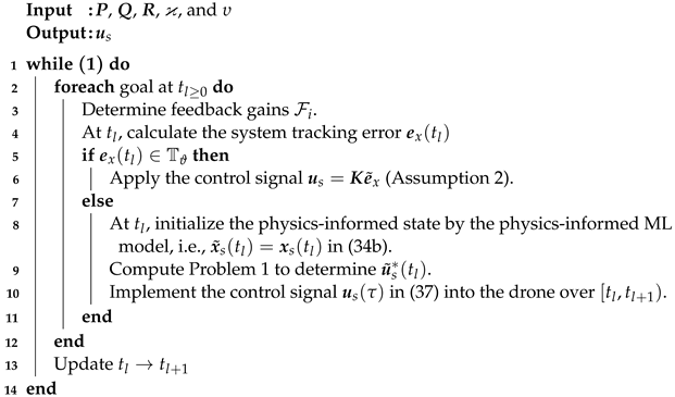
4. Comparative Analysis

4.1. Simulation Studies

The parameters of the aerial robot are provided as follows: m = 1.6 kg, I x x = I y y = 0.025 kg.m 2 , I z z = 0.005 kg.m 2 , l 1 = 0.17 m, l 2 = 0.06 m, g = 9.8 m/s 2 . 30% parametric uncertainty for the entire flight is considered during the simulation study. To validate the reliability of the controller, a high-speed υ = 20 m/s is selected for the comparative analysis. In the cost function, R = diag { 0.1 0.1 0.1 0.1 1 1 } , and the values of q i and p i are 1 and 0.25, respectively. In Problem 1, the numerical values of t p , t i , ϑ , F i , ϖ and ϰ are chosen as 10 s, 0.05 s, 0.04, 4, 0.08 and 0.2, respectively. λ is selected as 0.02, 0.03, 0.04, 0.042, 0.05, 0.051, 0.06, 0.07, 0.08, 0.085, 0.09, and 0.095. The constraints are 1 ξ I 1 , 2.5 V I 2.5 , 0 T 4 , π / 4 Θ π / 4 , and 2 ω B 2 .
In order to corroborate the control performance, different trajectories are defined that show that the DFAV has the properties of fixed-wing aircraft and helicopters. Suppose the drone is flying with an angular velocity of 2 rad/s. In the first trajectory (65), the aircraft takes off, and after attaining a certain altitude, it performs a bank-turn motion:
ξ x = sin ( 2 t ) , ξ y = 5 cos ( 2 t ) , ξ z = 50 e 3 t .
In the second instance, we validate the control performance with a helical 3D trajectory:
ξ x = sin ( 2 t ) , ξ y = 5 cos ( 2 t ) , ξ z = 50 t cos ( 2 t ) .
Moreover, since the aerial robot is flying with high speed υ , we validate the performance with a straight and level flight (SLF), a kind of horizontal flight phase of DFAVs [14]. During this flight, the drone must keep a constant altitude (e.g., 40 m) during the entire time, while the aircraft should fly at the desired angles, i.e., α = 5 and θ = 5 . In this case, some initial conditions are required to be considered, e.g., ξ x ( 0 ) = 0 m, ξ z ( 0 ) = 39 m, α ( 0 ) = 4 . 8 , and θ ( 0 ) = 4 . 8 .
Three different cases are considered:
  • Case (1): Performance in the presence of parametric uncertainties;
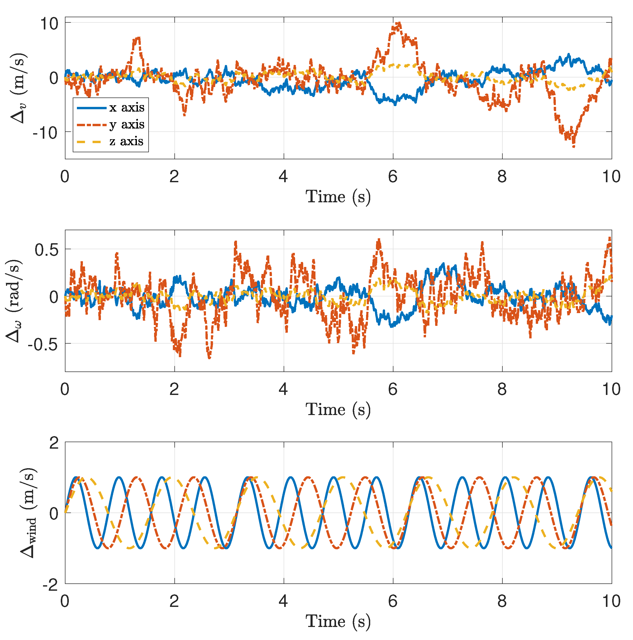
  • Case (2): Performance in the presence of parametric uncertainties and disturbances;
  • Case (3): Performance in the presence of faults, model uncertainties and disturbances.
Before proceeding to the aforementioned case studies, the correlation between flight performance and endurable wind speed is provided. In the previous work based on this aerial vehicle [47], aircraft was flown at various speeds under different weather conditions. From these real-time experiments, it was found that the maximum endurable wind speed is approximately 8 m/s. Therefore, it can be concluded that effective flight performance can be achieved if the wind speed is within the maximum endurable wind speed limit. However, the flight performance degrades as the wind speed passes the maximum endurable wind speed threshold. If the aircraft keeps flying over this maximum endurable wind speed, it encounters a structural failure, or a severe fault may occur. Nonetheless, the severity of this structural failure or fault depends on the magnitude and the total duration of the wind gust it encounters. To keep in view the contributions and main objective of this article, we deal with the control performance only under three case studies, under calm weather (Case 1), and wind gust is present (Case 2). However, it is assumed that it may not cause any structural faults because the magnitude of the wind gust is mostly under 8 m/s during the entire flight. Lastly, it is considered in the third case study that the partial fault exists associated with the unavailability of the dynamical information of the wings whose probability of occurrence is less than 3%. This occurrence level is uncommon, but to precisely verify the efficacy of the control approach, the worst-case situation (less than 3%) shall be analyzed in the third case study.

4.1.1. Case(1): Trajectory Tracking Response under Model Uncertainties

A comparative analysis of both strategies under model uncertainties is shown in Figure 5. In Figure 5a, the simulation results based on 3D trajectory (65) and (66) are illustrated. Furthermore, the tracking response under model inaccuracies derived from SLF flight is depicted in Figure 5b. Both controllers are primarily constructed on the principle of nominal MPC with similar attributes, so they exhibit adequate tracking performance. Nevertheless, the proposed technique demonstrates effective control performance with fast response and rapid convergence time.

4.1.2. Case(2): Trajectory Tracking Response under Uncertainties and Disturbances

Recall disturbance model in (29): the continuous Dryden wind turbulence model MIL-HDBK-1797B is employed using Simulink with default parameters chosen. Due to some minor limitations in this turbulence model, wind components are added, depicted in Figure 6. These wind components are composed of sinusoidal waveform Δ wind = [ sin ( 8 t ) sin ( 6.01 t ) sin ( 4.02 t ) ] T . The trajectory tracking performance under model uncertainties and disturbances are shown in Figure 7. Note that the MPC-CFC performance, as opposed to the developed approach, deteriorates despite having a dedicated DOB mechanism. This conclusively indicates that DOB in MPC-CFC [16,17] is only suitable for slow time-varying disturbances.

4.1.3. Case(3): Tracking Response in the Presence of Model Uncertainties, Disturbances, and Fault

In the third case study, suppose a fault occurs during the initial few seconds of the simulations due to the presence of a strong wind gust, considered in (29), and this fault is considered as a partial malfunction in one of the wings of the aircraft, whose role is depicted in Figure 2, is now either unavailable or unknown in this case. The tracking performance subject to disturbances, uncertainties, and fault is shown in Figure 8. More specifically, this fault has an adverse effect while controlling the attitude of the aerial platform illustrated in Figure 8b. In this aspect, as adaptive SINDY is equipped to handle and compensate for model divergence and correction, unlike DOB developed offline in [16,17], the presented approach by exploiting the full potential of MPC reveals effective control performance compared to the MPC-CFC technique [16,17].

4.1.4. Performance Analysis Based on Tracking Error and Computations

To analyze the effectiveness of both techniques, mean absolute error (MAE) is utilized and is defined as follows:
MAE = j = 1 n obs | e ( t j ) | / n obs ,
where e ( t j ) and n obs are the tracking error in each time step and the sum of a number of observations, respectively. In Table 2, a comparative analysis is illustrated. The trajectory error suggests that the designed approach shows effective tracking performance.
The numerical simulations are executed on Windows-driven Intel-based dual-core processor (2.2 GHz) with 8 GB of RAM. The optimization Problem 1 is written in MATLAB 2021a via CasADi [48], 3.5.5 version, and computed by NLP solver IPOPT [49], 3.12.3 version. The computational cost of these schemes is determined by the time required to compute the control action during the trajectory tracking response, depicted in Figure 9. Based on these findings, the average normalized computational time for the entire simulation study for the developed algorithm and MPC-CFC strategy is 18.62 ms and 19.51 ms, respectively.

4.2. Discussion

Different case studies have shown that the developed algorithm demonstrates an efficient tracking performance compared to the MPC-CFC technique. It is primarily due to the hybrid modeling approach integrated with the control mechanism that enables the MPC-based controller to perform effectively despite uncertainties, disturbances, and faults. This also confirms our earlier assertion that physics-informed dynamics and DOB in the disturbance rejection MPC approaches (e.g., [16,17]) limited the capability of MPC due to inadequate modeling and ineffective estimation. Nevertheless, the computational complexity may be affected if a large amount of data are utilized online rather than with less data. With regard to the ML technique related to adaptive SINDy, this work has not addressed any shortcomings concerning this method (e.g., noise sensitivity and long-term memory), as they are beyond the scope of this article. Regarding flight robustness, the proposed framework is designed based on a more suitable selection of the terminal region, which yields adequate stability margins as opposed to [16,17]. In spite of all the aforementioned benefits, the presented MPC-based technique using a physics-informed ML model still ensures sub-optimal performance.

5. Conclusions and Future Directions

This paper has presented an MPC-based control design for the ducted fan aircraft utilizing a hybrid modeling scheme known as physics-informed ML. In the beginning, the physics-informed model was derived offline from the drone with sufficient capabilities. Thereafter, an online-based data-driven modeling technique is integrated with physics-informed dynamics to determine the actual model. Afterwards, an MPC-based control algorithm was developed by updating the physics-informal dynamics (nominal system) with real states. ISS stability and recursive feasibility were proven under adequate conditions. Finally, simulations were conducted under three different scenarios starting from challenging (case 1), worse (case 2), and worst-case situation (case 3), which revealed that the developed framework exhibits effective control performance.
For future studies, the worst-case scenario can be utilized as a baseline to effectively construct a more refined fault-tolerant controller. Nevertheless, it is noteworthy that the developed framework is not designed as a fault-tolerant controller. Moreover, the worst-case scenario is only verified under a partial fault occurrence. Furthermore, the designed strategy also ensures sub-optimal performance like [16,17] for aerial applications.
In the end, several future directions can be pursued to improve the efficacy of the proposed strategy:
  • Physics-informed modeling: the designed model is basically derived from the principle of the Newton–Euler method. Other mathematical models, such as the Lagrange-Euler approach, can be employed;
  • Data-driven ML: the developed ML scheme was inspired by adaptive SINDy [30], where different ways of improving the ML model’s capability can be explored. Moreover, further investigation is required to find an effective technique to enhance computational efficiency with more data and less physics;
  • Real-time implementation: future work will involve real-time testing of the presented framework. For this purpose, a more suitable solver can be used for code generation especially developed for real-time embedded optimization.

Author Contributions

Conceptualization, T.M.; methodology, T.M., Z.S. and Z.C.; software, T.M.; validation, T.M.; formal analysis, T.M., Z.S. and H.P.; investigation, T.M.; resources, H.P.; data curation, T.M. and Z.C.; writing—original draft preparation, T.M.; writing—review and editing, T.M., Z.S., Z.C. and H.P.; visualization, T.M., Z.S., Z.C. and H.P.; supervision, H.P.; project administration, H.P.; funding acquisition, T.M. and H.P. All authors have read and agreed to this version of the manuscript.

Funding

This work was supported in part by the Scientific Instruments Development Program of NSFC of China: 615278010, in part by Fundamental Research Funds for the Central Universities, in part by Science and Technology Planning Project of Guangdong, China: 2017B010116005, and in part by 2022 Foreign Expert Program (Foreign Youth Talent Program) of Ministry of Science and Technology of China: QN2022163002.

Institutional Review Board Statement

Not applicable.

Informed Consent Statement

Not applicable.

Data Availability Statement

The data presented in this article are available on reasonable request from the authors.

Acknowledgments

The authors would like to thank all the funders who supported this work.

Conflicts of Interest

The authors declare no conflict of interest.

Abbreviations

The following abbreviations are used in this manuscript:
DFAVDucted Fan Aerial Vehicle
DOBDisturbance Observer
MPCModel Predictive Control
MPC-CFCMPC-based Compound Flight Control
MAEMean Absolute Error
MLMachine Learning
NNNeural Network
SINDySparse Identification of Nonlinear Dynamics
SLFStraight and Level Flight

References

  1. Cheng, Z.; Pei, H. Control Effectiveness Enhancement for the Hovering/Cruising Transition Control of a Ducted Fan UAV. J. Intell. Robot. Syst. 2022, 105. [Google Scholar] [CrossRef]
  2. Cheng, Z.; Pei, H. Transition Analysis and Practical Flight Control for Ducted Fan Fixed-Wing Aerial Robot: Level Path Flight Mode Transition. IEEE Robot. Autom. Lett. 2022, 7, 3106–3113. [Google Scholar] [CrossRef]
  3. Cheng, Z.; Pei, H. Flight Transition Control for Ducted Fan UAV with Saturation on Control Surfaces. In Proceedings of the 2021 International Conference on Unmanned Aircraft Systems (ICUAS), Athens, Greece, 5–18 June 2021; pp. 439–446. [Google Scholar] [CrossRef]
  4. Marconi, L.; Naldi, R.; Gentili, L. Modelling and control of a flying robot interacting with the environment. Automatica 2011, 47, 2571–2583. [Google Scholar] [CrossRef] [Green Version]
  5. Naldi, R.; Macchelli, A.; Mimmo, N.; Marconi, L. Robust Control of an Aerial Manipulator Interacting with the Environment. IFAC-PapersOnLine 2018, 51, 537–542. [Google Scholar] [CrossRef]
  6. Marconi, L.; Naldi, R. Control of Aerial Robots: Hybrid Force and Position Feedback for a Ducted Fan. IEEE Control Syst. Mag. 2012, 32, 43–65. [Google Scholar] [CrossRef]
  7. Naldi, R.; Torre, A.; Marconi, L. Robust Control of a Miniature Ducted-Fan Aerial Robot for Blind Navigation in Unknown Populated Environments. IEEE Trans. Control Syst. Technol. 2015, 23, 64–79. [Google Scholar] [CrossRef]
  8. Roberts, A.; Tayebi, A. Adaptive position tracking of VTOL UAV. IEEE Trans. Robot. 2011, 27, 129–142. [Google Scholar] [CrossRef] [Green Version]
  9. Manzoor, T.; Xia, Y.; Ali, Y.; Hussain, K. Flight control techniques and classification of ducted fan aerial vehicles. Kongzhi Lilun Yu Yingyong/Control Theory Appl. 2022, 39, 201–221. [Google Scholar] [CrossRef]
  10. Hua, M.; Hamel, T.; Morin, P.; Samson, C. Introduction to feedback control of underactuated VTOL vehicles: A review of basic control design ideas and principles. IEEE Control Syst. Mag. 2013, 33, 61–75. [Google Scholar] [CrossRef]
  11. Eren, U.; Prach, A.; Kocer, B.; Rakovic, S.V.; Kayacan, E.; Acikmese, B. Model Predictive Control in Aerospace Systems: Current State and Opportunities. J. Guid. Control. Dyn. 2017, 40, 1541–1566. [Google Scholar] [CrossRef]
  12. Banazadeh, A.; Emami, S.A. Control effectiveness investigation of a ducted-fan aerial vehicle using model predictive controller. In Proceedings of the 2014 International Conference on Advanced Mechatronic Systems, Kumamoto, Japan, 10–12 August 2014; pp. 532–537. [Google Scholar] [CrossRef]
  13. Emami, A.; Banazadeh, A. Robustness investigation of a ducted-fan aerial vehicle control, using linear, adaptive, and model predictive controllers. Int. J. Adv. Mechatron. Syst. 2015, 6, 108–117. [Google Scholar] [CrossRef]
  14. Manzoor, T.; Xia, Y.; Zhai, D.H.; Ma, D. Trajectory tracking control of a VTOL unmanned aerial vehicle using offset-free tracking MPC. Chin. J. Aeronaut. 2020, 33, 2024–2042. [Google Scholar] [CrossRef]
  15. Emami, A.; Rezaeizadeh, A. Adaptive model predictive control-based Attitude and Trajectory Tracking of a VTOL Aircraft. IET Control Theory Appl. 2018, 12, 2031–2042. [Google Scholar] [CrossRef]
  16. Manzoor, T.; Sun, Z.; Xia, Y.; Ma, D. MPC based compound flight control strategy for a ducted fan aircraft. Aerosp. Sci. Technol. 2020, 107, 106264. [Google Scholar] [CrossRef]
  17. Manzoor, T.; Pei, H.; Cheng, Z. Composite observer-based robust model predictive control technique for ducted fan aerial vehicles. Nonlinear Dyn. 2022. [Google Scholar] [CrossRef]
  18. Hewing, L.; Wabersich, K.P.; Menner, M.; Zeilinger, M.N. Learning-Based Model Predictive Control: Toward Safe Learning in Control. Annu. Rev. Control. Robot. Auton. Syst. 2020, 3, 269–296. [Google Scholar] [CrossRef]
  19. Brunke, L.; Greeff, M.; Hall, A.W.; Yuan, Z.; Zhou, S.; Panerati, J.; Schoellig, A.P. Safe Learning in Robotics: From Learning-Based Control to Safe Reinforcement Learning. Annu. Rev. Control. Robot. Auton. Syst. 2022, 5, 411–444. [Google Scholar] [CrossRef]
  20. Kaheman, K.; Kaiser, E.; Strom, B.; Kutz, J.N.; Brunton, S.L. Learning Discrepancy Models From Experimental Data. arXiv 2019, arXiv:1909.08574. [Google Scholar] [CrossRef]
  21. Brunton, S.L.; Kutz, J.N. Data-Driven Science and Engineering: Machine Learning, Dynamical Systems, and Control; Cambridge University Press: Cambridge, UK, 2019. [Google Scholar] [CrossRef] [Green Version]
  22. Brunton, S.L.; Nathan Kutz, J.; Manohar, K.; Aravkin, A.Y.; Morgansen, K.; Klemisch, J.; Goebel, N.; Buttrick, J.; Poskin, J.; Blom-Schieber, A.W.; et al. Data-Driven Aerospace Engineering: Reframing the Industry with Machine Learning. AIAA J. 2021, 59, 2820–2847. [Google Scholar] [CrossRef]
  23. Zhang, W.; Shen, J.; Ye, X.; Zhou, S. Error model-oriented vibration suppression control of free-floating space robot with flexible joints based on adaptive neural network. Eng. Appl. Artif. Intell. 2022, 114, 105028. [Google Scholar] [CrossRef]
  24. Hosseini, S.; Poormirzaee, R.; Hajihassani, M. Application of reliability-based back-propagation causality-weighted neural networks to estimate air-overpressure due to mine blasting. Eng. Appl. Artif. Intell. 2022, 115, 105281. [Google Scholar] [CrossRef]
  25. Floriano, B.R.; Vargas, A.N.; Ishihara, J.Y.; Ferreira, H.C. Neural-network-based model predictive control for consensus of nonlinear systems. Eng. Appl. Artif. Intell. 2022, 116, 105327. [Google Scholar] [CrossRef]
  26. Park, B.S.; Yoo, S.J. Quantized-communication-based neural network control for formation tracking of networked multiple unmanned surface vehicles without velocity information. Eng. Appl. Artif. Intell. 2022, 114, 105160. [Google Scholar] [CrossRef]
  27. Kaiser, E.; Kutz, J.N.; Brunton, S.L. Sparse identification of nonlinear dynamics for model predictive control in the low-data limit. Proc. R. Soc. A Math. Phys. Eng. Sci. 2018, 474, 20180335. [Google Scholar] [CrossRef] [PubMed] [Green Version]
  28. Brunton, S.L.; Proctor, J.L.; Kutz, J.N. Discovering governing equations from data by sparse identification of nonlinear dynamical systems. Proc. Natl. Acad. Sci. USA 2016, 113, 3932–3937. [Google Scholar] [CrossRef] [PubMed] [Green Version]
  29. Cao, R.; Lu, Y.; He, Z. System identification method based on interpretable machine learning for unknown aircraft dynamics. Aerosp. Sci. Technol. 2022, 126, 107593. [Google Scholar] [CrossRef]
  30. Quade, M.; Abel, M.; Nathan Kutz, J.; Brunton, S.L. Sparse identification of nonlinear dynamics for rapid model recovery. Chaos: Interdiscip. J. Nonlinear Sci. 2018, 28, 063116. [Google Scholar] [CrossRef]
  31. Karniadakis, G.E.; Kevrekidis, I.G.; Lu, L.; Perdikaris, P.; Wang, S.; Yang, L. Physics-informed machine learning. Nat. Rev. Phys. 2021, 3, 422–440. [Google Scholar] [CrossRef]
  32. Arnold, F.; King, R. State–space modeling for control based on physics-informed neural networks. Eng. Appl. Artif. Intell. 2021, 101, 104195. [Google Scholar] [CrossRef]
  33. Zobeiry, N.; Humfeld, K.D. A physics-informed machine learning approach for solving heat transfer equation in advanced manufacturing and engineering applications. Eng. Appl. Artif. Intell. 2021, 101, 104232. [Google Scholar] [CrossRef]
  34. Shen, S.; Lu, H.; Sadoughi, M.; Hu, C.; Nemani, V.; Thelen, A.; Webster, K.; Darr, M.; Sidon, J.; Kenny, S. A physics-informed deep learning approach for bearing fault detection. Eng. Appl. Artif. Intell. 2021, 103, 104295. [Google Scholar] [CrossRef]
  35. Liu, X.; Peng, W.; Gong, Z.; Zhou, W.; Yao, W. Temperature field inversion of heat-source systems via physics-informed neural networks. Eng. Appl. Artif. Intell. 2022, 113, 104902. [Google Scholar] [CrossRef]
  36. Nascimento, R.G.; Fricke, K.; Viana, F.A. A tutorial on solving ordinary differential equations using Python and hybrid physics-informed neural network. Eng. Appl. Artif. Intell. 2020, 96, 103996. [Google Scholar] [CrossRef]
  37. Ahnert, K.; Abel, M. Numerical differentiation of experimental data: Local versus global methods. Comput. Phys. Commun. 2007, 177, 764–774. [Google Scholar] [CrossRef]
  38. Chartrand, R. Numerical Differentiation of Noisy, Nonsmooth Data. Int. Sch. Res. Netw. 2011, 2011, 1023–1033. [Google Scholar] [CrossRef] [Green Version]
  39. Zhang, L.; Schaeffer, H. On the Convergence of the SINDy Algorithm. Multiscale Model. Simul. 2019, 17, 948–972. [Google Scholar] [CrossRef] [Green Version]
  40. Gershenfeld, N.A. The Nature of Mathematical Modeling; Cambridge University Press: Cambridge, UK, 1999. [Google Scholar] [CrossRef]
  41. Xue, R.; Dai, L.; Huo, D.; Xie, H.; Sun, Z.; Xia, Y. Compound tracking control based on MPC for quadrotors with disturbances. J. Frankl. Inst. 2022, 359, 7992–8013. [Google Scholar] [CrossRef]
  42. Chen, H.; Allgöwer, F. A Quasi-Infinite Horizon Nonlinear Model Predictive Control Scheme with Guaranteed Stability. Automatica 1998, 34, 1205–1217. [Google Scholar] [CrossRef]
  43. Althoff, M.; Stursberg, O.; Buss, M. Reachability analysis of nonlinear systems with uncertain parameters using conservative linearization. In Proceedings of the 47th IEEE Conference on Decision and Control, Cancun, Mexico, 9–11 December 2008; pp. 4042–4048. [Google Scholar] [CrossRef] [Green Version]
  44. Sun, Z.; Xia, Y. Receding horizon tracking control of unicycle-type robots based on virtual structure. Int. J. Robust Nonlinear Control 2016, 26, 3900–3918. [Google Scholar] [CrossRef]
  45. Sontag, E.D. Input to State Stability: Basic Concepts and Results. In Nonlinear and Optimal Control Theory: Lectures Given at the C.I.M.E. Summer School Held in Cetraro, Italy June 19–29, 2004; Springer: Berlin/Heidelberg, Germany, 2008; pp. 163–220. [Google Scholar] [CrossRef]
  46. Sun, Z.; Dai, L.; Liu, K.; Xia, Y.; Johansson, K.H. Robust MPC for tracking constrained unicycle robots with additive disturbances. Automatica 2018, 90, 172–184. [Google Scholar] [CrossRef]
  47. Cheng, Z.; Pei, H.; Li, S. Neural-Networks Control for Hover to High-Speed-Level-Flight Transition of Ducted Fan UAV With Provable Stability. IEEE Access 2020, 8, 100135–100151. [Google Scholar] [CrossRef]
  48. Andersson, J.A.E.; Gillis, J.; Horn, G.; Rawlings, J.B.; Diehl, M. CasADi–A software framework for nonlinear optimization and optimal control. Math. Program. Comput. 2019, 11, 1–36. [Google Scholar] [CrossRef]
  49. Wächter, A.; Biegler, L.T. On the implementation of an interior-point filter line-search algorithm for large-scale nonlinear programming. Math. Program. 2006, 106, 25–57. [Google Scholar] [CrossRef]
Figure 1. Physics and data scenario in the presented scheme.
Drones 07 00004 g001
Figure 2. (a) Inertial and body-fixed frame; (b) other components during flight; (c) aerodynamic effects on the duct; (d) aerodynamic effects on the wings.
Drones 07 00004 g002
Figure 3. Physics-informed ML model for DFAVs.
Drones 07 00004 g003
Figure 4. Schematic diagram of the MPC-based control approach using physics-informed ML.
Drones 07 00004 g004
Figure 5. Tracking response under model uncertainties (a) 3D trajectory tracking (b) SLF flight.
Drones 07 00004 g005
Figure 6. Disturbance profile involving Dryden wind turbulence ( Δ w , Δ v ) and other time-varying wind disturbances Δ wind .
Drones 07 00004 g006
Figure 7. Tracking response under uncertainties and disturbances (a) 3D trajectory tracking; (b) SLF flight.
Drones 07 00004 g007
Figure 8. Tracking response under model uncertainties, disturbances, and fault (a) 3D trajectory tracking; (b) SLF flight.
Drones 07 00004 g008
Figure 9. Normalized computational time of both frameworks.
Drones 07 00004 g009
Table 1. A concise comparison between existing MPC-based control methods and the proposed technique for DFAVs (order by year).
ReferencesFeatures 1AdvantagesDisadvantages
Linear MPC [12,13]AMSSimple design, effectiveLack adequate tracking and robustness.
computations.
1. Disturbance rejection RMPC 2,ACDMPSConsidered time-delays, discrete time optimization problem1. RMPC 2: lack effective control performance,
2. Disturbance rejection adaptive 2. Adaptive MPC: design intricacy may not be effective, feasibility analysis is not available for both schemes.
Observer-based MPC [14]ACDMPSEffective computations, easy real-time implementation, considered time delays.Ineffective control performance, recursive easibility cannot be established for the entire flight.
Compound RMPC 2 [16,17]ACDMPS-Inadequate performance, suitable if the DOB’s dynamics is faster than disturbance dynamics.
1 A: attitude tracking, C: composite technique, D: DOB, M: physics-informed modeling, P: position tracking, S: simulation study. 2 RMPC: Robust MPC.
Table 2. Performance analysis based on tracking error (MAE).
ScenarioMPC-CFCProposed ScenarioMPC-CFCProposed
ξ y (m)Case(1)-Figure 5a1.57520.0016 ξ z (m)Case(1)-Figure 5b0.17110.1424
Case(1)-Figure 5a0.15690.0157Case(1)-Figure 5a0.00111.09 × 10 6
Case(2)-Figure 7a2.32790.0141Case(2)-Figure 7b0.09990.0987
Case(2)-Figure 7a0.23570.0235Case(2)-Figure 7a0.00169.82 × 10 6
Case(3)-Figure 8a2.86870.0157Case(3)-Figure 8b0.1220.0782
Case(3)-Figure 8a0.47290.0314Case(3)-Figure 8a0.0021.091 × 10 5
ξ x (m)Case(1)-Figure 5a0.030660.0003 θ ( ° )Case(1)-Figure 5b0.04820.0378
Case(1)-Figure 5a0.03250.0033Case(2)-Figure 7b0.03760.0349
Case(2)-Figure 7a0.44290.0029Case(3)-Figure 8b0.07480.0284
Case(2)-Figure 7a0.04860.049 α ( ° )Case(1)-Figure 5b0.04660.0460
Case(3)-Figure 8a0.54460.0033Case(2)-Figure 7b0.03710.0344
Case(3)-Figure 8a0.09660.0065Case(3)-Figure 8b0.0690.0389
Disclaimer/Publisher’s Note: The statements, opinions and data contained in all publications are solely those of the individual author(s) and contributor(s) and not of MDPI and/or the editor(s). MDPI and/or the editor(s) disclaim responsibility for any injury to people or property resulting from any ideas, methods, instructions or products referred to in the content.

