Abstract
In this paper, the consensus control of unmanned surface vehicles (USVs) is investigated by employing a distributed model predictive control approach. A hierarchical control structure is considered during the controller design, where the upper layer determines the reference signals of USV velocities while the lower layer optimizes the control inputs of each USV. The main feature of this work is that a post-verification procedure is proposed to address the failure states caused by local errors or cyberattacks. Each USV compares the actual state and the predicted one obtained at the previous moment. This allows the estimation of local perturbations. In addition, the failure state of the USV can also be determined if a preset condition is satisfied, thus forcing a change in the communication topology and avoiding further impact. Simulations show that the proposed method is effective in USV formation control. Compared with the method without post-verification, the proposed approach is more robust when failure states occur.
1. Introduction
In recent years, the cooperative control of unmanned surface vehicles (USVs) has attracted considerable attention in systems and ocean engineering fields, broadening their applications in territorial surveillance, marine rescue, environmental detection, etc. When USVs cooperate as a formation [1], they can improve efficiency, reduce costs and switch the communication topology to provide redundancy in the event of the failure of any single USV. Formation control mainly solves two problems, namely formation composition and formation maintenance. Formation maintenance is the core feature of formation control, and is the main task of the USV navigation stage. The currently available formation control methods are primarily based on the leader–follower strategy [2,3], behavior-based method [4,5] and virtual structure method [6,7,8,9,10].
Among these control schemes, the leader–follower strategy has garnered more practical attention due to its simplicity and practicality; the collaborative control of USVs has been reported in many excellent works under the framework of a leader–follower strategy. In [11], to address the formation control problem of underactuated USVs, consistency theory and the leader–follower method were used along with the adjustment of the control input such that each USV converged to the reference value, thereby ensuring the expected formation of the USVs. Park and Yoo [12] deduced the performance functions of connection maintenance and collision avoidance for a nonlinear USV model, and completed a robust leader–follower formation tracking design. In [13], under the influences of USV input overload and external interference, the back-stepping method was used to improve formation control accuracy.
Formation control is generally divided into three categories based on the control method under the leader–follower strategy: centralized [14,15,16], decentralized [17,18,19,20,21] and distributed control [22]. In centralized control, there is a need to collect all information from USVs, and the large scale of the system increases the burden of online computing, which makes it more difficult to ensure real-time performance. Different from centralized control, decentralized control has no information exchange between the controllers, and coupling is ignored such that the vehicles may not achieve cooperative control in most cases. Distributed control allows full autonomy of the USVs, in addition to having the characteristics of low computational burden, strong fault tolerance, robustness and scalability; hence, this formation control method is more suitable for large-scale systems with a greater number of nodes, and it has attracted significant attention from scientists and researchers [23,24,25,26,27].
Although great progress has been achieved in the distributed formation control of USVs, the problem involves multi-input, multi-output systems with constraints and coupled tasks, making it inherently difficult [28,29,30,31,32]. Fortunately, distributed model predictive control (DMPC) has significant advantages in handling this class of problems [33,34]. The DMPC method combines model predictive control and distributed control principles organically, and is thus robust and flexible [35,36]. Hence, it is an ideal tool for USV formation control. DMPC has been used to investigate the formation control of vehicles. Zhao et al. [37] proposed a DMPC method for multi-quadrotor unmanned aerial vehicles (UAVs) to address the formation and maintenance problem during a cruise flight. The cost function was designed by introducing the assumed state trajectories of the local vehicle and its neighbors. Zhen et al. [38] presented a DMPC approach for vehicle platoons with one-way topologies. The terminal constraint based on the adjacent average value was introduced into the cost function, and then the closed-loop stability was proved. Zhao et al. [39] proposed a novel distributed coordinated control scheme on the grounds of heterogeneous UAVs to achieve formation control. Further results were reported by Fan et al. [40], who proposed a formation control strategy based on a hierarchical DMPC strategy, in which the upper layer guarantees the leader–follower cooperation between the unmanned vessels while the lower layer allows the unmanned vessels to track optimal instructions. Note that DMPC employs a receding horizon optimization during the implementation, which provides distributed agents with local prediction capabilities; in other words, “assumed” states are available to each agent. The assumed states play important roles in the formation control. They reflect local disturbances, since the actual states usually differ from the assumed ones. Furthermore, some failure states caused by local errors or cyberattacks that are fatal to formation control may also be determined if local predictions can be fully utilized. These have not been well studied in the existing literature, and thus motivated our research. In this paper, a hierarchical DMPC approach with post-verification is proposed for USVs with actuation constraints. Since the inputs of USVs are usually not coupled, the upper layer mainly considers communication interactions between USVs and generates the optimal references for the lower layer according to the kinematic model. The lower layer predictive controller is designed based on the dynamic model to ensure the tracking performance. The local predictions are employed in three aspects. First, the states within the prediction horizon are sent to the neighbors for the purpose of formation control. Second, the assumed states of a USV are incorporated in its local cost function, which improves its control performance when local disturbances exist. Third, the differences between the actual states and the assumed states are sent to the neighbor in the post-verification process, which renders compensations for the local predictions to be used by the neighbors. Moreover, failure states are determined once the differences satisfy a preset condition, in which case the communication topology is forced to change to an alternative one, where the affected USV does not send information to other agents. In this way, the USVs can still maintain the desired formation, avoiding the phenomenon of formation disorder caused by failure states. Under the directed and time-invariant communication topology, the upper-layer controller was considered based on the kinematic model of the USV to generate the optimal references and the lower-layer controller was designed using the dynamic model to ensure the tracking performance. By comparing the actual state with the predicted state obtained at the previous time, the post-verification process can reduce the trajectory deviation caused by external disturbances, which can increase the speed of forming the required formation. In this study, a backup topology is also designed. When the post-verification process meets the preset conditions, it is judged that the communication information between the two USVs (communicating according to communication topology ) is wrong or interrupted. At this time, the topology is forced to change from the normal state to the fault state, so that the USVs can keep the desired formation while tracking their respective expected paths, improving the phenomenon of formation disorder due to communication failures.
The main features of the proposed approach are summarized as follows.
- The USV formation control method has strong robustness with respect to external disturbances. This is because the local predictions are used by both the single USV and its neighbors in constructing cost functions. Therefore, it is suitable for USVs that operate in extreme conditions, such as strong winds.
- The proposed approach can deal with fatal errors that exist in a single USV or at the communication level, since the post-verification process compares the actual states with the assumed ones, which enable it to determine the failure states in time, reducing the formation error and maintaining the formation shape. Although USVs can be equipped with advanced communication technologies [41,42], it is still important to adapt active fault-tolerant control strategies.
The remainder of this manuscript is organized as follows. In Section 2, the mathematical models of a single USV and the formation system are established; in Section 3, the predictive formation control strategies of the upper DMPC-based and lower MPC-based controllers are introduced; in Section 4, the algorithmic flow of the control strategy is presented; Section 5 shows the simulation examples; in Section 6, a summary of this work is provided.
2. Problem Statement
2.1. Modeling of USV
Consider a group of multiple USVs, labeled 1 to 6. For each USV, the kinematic model is expressed as follows:
where is the position and is the heading angle of each USV. The vector is defined as , where is the linear velocity on the X- and Y-axes, and is the angular velocity of the rudder. is the inertia matrix including added mass; the matrix is the Coriolis and centripetal forces and moments; the matrix is the fluid damping matrix. The vector is the control input corresponding to propeller thrust and the rudder deflection angle; the matrix is a matrix. The dynamic model of each USV is stated as follows:
where are the hydrodynamic forces and moment; and are rudder coefficients connected with speed and yaw moment, respectively; m and are the vehicle mass and mass moment of inertia, respectively; and are the rudder deflection angle and propeller thrust, respectively; u and v are the linear velocities (X-axis and Y-axis), and r is the angular velocity; and and are time-invariant current disturbances: , .
2.2. Communication Topology
The directed graph is used to describe the communication topology of the formation system, where represents the set of nodes in the graph ; represent the set of edges. is the set of time-varying adjacency matrix, which describes the communication among the followers. Edge represents that node i is able to obtain the status information of node j, and we say that node j is the neighbor of node i. If , then ; otherwise, . Using to represent the neighbor set of node i, is used to represent the collection of nodes that can obtain the information about node i. The Laplacian matrix is defined as , where is named the degree matrix, and defined as with .
2.3. Control Objective of Multi-USV Systems
Considering the desired formation control problem as demonstrated in Figure 1, USV is the leader ship, USV− USV are the follower ships and each USV follows a preset formation. The formation requirements are as follows: (1) each USV tracks a provided straight trajectory; (2) according to the formation matrix, the distance between USVs can be calculated, and the specific formation matrix is defined in the simulation example; (3) each USV can exchange position information with the adjacent USVs via communication networks; (4) if any communication networks fail, standby communication networks can be quickly switched to maintain the desired formation.
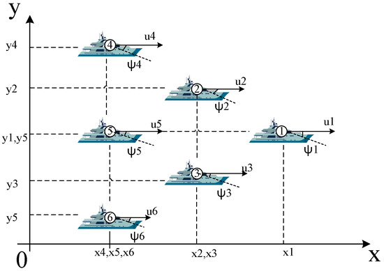
Figure 1.
Illustration of a desired formation motion.
3. Design of Distributed Model Predictive Controller
This section first introduces the controllers used by the upper and lower structures of the formation system; the upper layer has a DMPC-based controller designed using the kinematic model, and the lower layer has an MPC-based controller designed using the dynamic model for tracking the optimal control input of the upper layer, as shown in Figure 2. To facilitate the demonstration, six USVs are considered. The upper layer obtains the formation (i.e., triangle formation) through the communication topology. The distributed MPC scheme is used to solve for the optimal solution and provides formation commands to each USV. The task of the lower controller is to track formation commands and achieve optimal output.
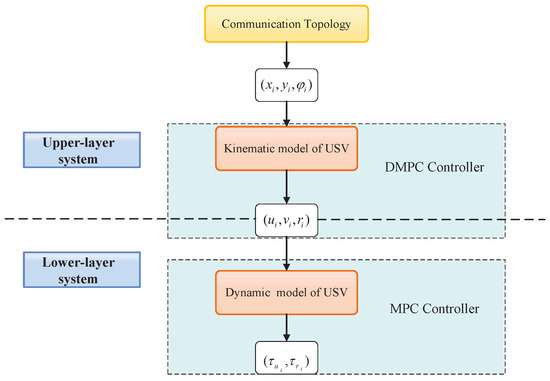
Figure 2.
Control structure.
3.1. Upper-Layer Distributed MPC
The same length of predictive horizon is used in all local problems. Over the prediction horizon , the used states and input symbols are listed in Table 1, where and the assumed state trajectory is essentially the optimal state trajectory obtained by solving the optimization problem at time .

Table 1.
States and input symbols.
Now we define the optimal control problem for each node at time t.
Problem :
subject to:
where denotes the unknown variables to be optimized; represents the set of neighbor states of the USV; constraint (5a) shows the constraint from USV kinematics; constraint (5b) indicates that the current state at time t is taken as the time initial state of the optimization problem; constraint (5c) denotes the control input set and , where and are the bounds; terminal equality constraint (5d) represents the terminal equality constraint of USV; and the state predicted by the last step at time t is equal to the desired state, which is mainly used to ensure the gradual stability of the system.
The function in (4) is the cost bounded with node i, defined as:
where , and and are the weighting matrices. In problem , the cost function (6) contains four items: (1) The first item corresponds to the penalty of the weight matrix for the deviation between the predicted state and the target state of USV, which represents the expectation of reaching the target state as soon as possible; present the target status of USV. (2) The second item corresponds to the penalty of the control input with the weight matrix , which represents that USV prefers uniform motion. is the desired speed, which is a constant. (3) The third item corresponds to the penalty of the weight matrix for the deviation (or self deviation for short) between the predicted track and the assumed track of USV. (4) The fourth item corresponds to the penalty for the deviation between the predicted track of USV and its neighbor’s assumed track., The offset is (or referred to as neighbor bias for short), and the weight matrix is , which indicates that USV should keep the expected bias running with the assumption state of neighbor nodes as much as possible. The third and fourth terms are called the self-bias penalty and neighbor-bias penalty, respectively, while and are called self-bias weight and neighbor-bias weight, respectively.
At the same time, all USVs in the formation system solve and update the optimization problems synchronously. From the above analysis, it is seen that the single-node optimization problem only uses the assumptions of neighboring node state information and that there is no global state information; thus, this is an innate problem of the distributed model predictive control scheme.
3.2. Lower-Layer MPC
After calculating by the DMPC formation controller, the optimal control input at time t for each USV will be achieved, and the lower-layer MPC controller will take optimal control input as the tracking reference . So, we define the lower-layer optimal control problem:
Problem :
subject to:
where denotes the unknown variables to be optimized; and are the predictive control input and predictive state trajectory of the lower-layer controller, respectively; constraint (8a) shows the constraint from USV dynamics; constraint (8b) represent the control input set and , where and are the bounds.
The function l in (7) is designed as:
where represents the intensity to penalize the output error from the desired state and represents the intensity to penalize the input error deviated from the desired state.
4. Implementation of the Algorithm
Based on the control strategy proposed above, the algorithm flow of the two-layer distributed model predictive control is as described in the following steps 1–5:
Step 1: According to the communication topology , all USVs are given the expected relative state information of other USVs.
Step 2: Initialization—at time , assuming that all USVs are in uniform motion during operation, for each USV take its current state as the initial value of the prediction state in the prediction time domain at this time, that is, , the assumed control inputs and assumed state are defined as
where ,
Step 3: At any time t, for each USV in the upper layer:
(1) Obtain the expected state trajectory of USV (leader ship) directly or indirectly according to the communication topology, and according to the pre-installed expected relative state information , solve the desired state trajectory .
(2) Optimize the problem according to its current state , self assumed state and neighbor assumed state trajectory, and obtain the optimal control input sequence .
(3) Calculate the optimal state trajectory within the prediction range using the optimal control sequence:
(4) Compute the assumed control for the next step by discarding the first term and adding one expected input term; the diagram of the synchronously updating algorithm is shown in Figure 3.
the corresponding assumed output is also calculated as:
i.e.,
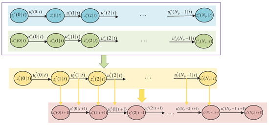
Figure 3.
Illustration of the upper-layer DMPC algorithm.
(5) According to the communication topology , the assumed state trajectory is sent to the USV that can receive its information, and at the same time, the assumed state trajectory of its neighbors is received.
(6) The first element of the optimal control sequence is used to implement the control effort, i.e., , conveying to its lower-layer control system as reference.
(7) Post-verification process: The error between the Y-axis outputs of the assumed and actual output states are obtained. Then, this error is compensated for the actual output of the system at the next moment. Considering the absolute value of the error , if , take cm in the simulation, it is considered that the communication information between USVs is determined to be wrong or interrupted. At this time, the communication topology changes from normal to error states.
Step 4: At any time t, for each USV in the lower-layer:
(1) Obtain the reference .
(2) Solve the optimization problem , yielding the optimal control sequence .
(3) Apply the first element of the optimal control sequence to the lower-layer control system. Calculate the optimal state trajectory within the prediction range using the optimal control sequence .
Step 5: At time , repeat the above steps.
5. Results and Discussion
5.1. Simulation Setup
The adopted communication topology is shown in Figure 4a. USV is selected as the leader, and the arrow indicates the signal transmission direction, that is, the information of the front-end USV (expected state trajectory, assumed state trajectory) can be obtained by the back-end USV. As shown in Figure 4b, when the communication between USV and USV fails, USV can receive signals from USV. As shown in Figure 4c, when the communication between USV and USV fails, USV can receive signals from USV and continue to move on in the desired formation.
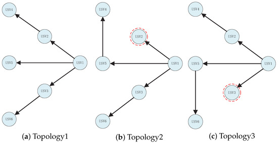
Figure 4.
Communication topologies. (a) Topology1 is a normal state. (b,c) Topology2 and Topology3 are failure states and red circles represent the faulty ships.
In the simulation, the system composed of six USV is equivalent to a homogeneous multi-agent system, so each USV has the same parameters, as follows: kg, , , , , , and . Table 2 lists the the initial state of USVs in the inertial system as well as the expected relative state between USVs, where , the first and second items of matrix mean the expected relative state information between USV and itself; similarly, the third and fourth items mean the expected relative state information between USV and USV, and so on. As the expected relative state between two UAVs can be obtained by , it is not listed.; the remaining simulation parameters are shown in Table 3. Theoretically, each USV can obtain its own expected state trajectory based on the expected relative state with other USVs. The maximum value of the control input of a USV in the kinematic model is and the minimum value is set to ; similarly, the maximum and minimum values of the control input of the USV in the dynamic model are set to and , respectively.
Table 2.
Initial and expected relative states.
Table 3.
Parameters used in the USV DMPC simulation.
5.2. Result Analysis
In order to verify that the algorithm can complete the first three control objectives proposed in Section 1, we ran the control algorithm designed in this paper to obtain Figure 5, Figure 6, Figure 7, Figure 8 and Figure 9. From these figures, it can be seen that the algorithm designed in this paper could achieve the desired control objectives, which verifies the effectiveness of the algorithm.
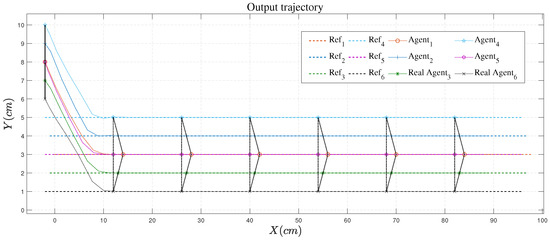
Figure 5.
Output trajectory.
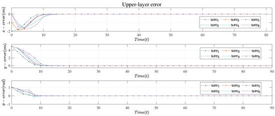
Figure 6.
Upper−layer error.
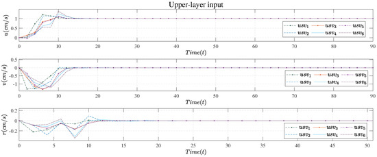
Figure 7.
Upper−layer input.
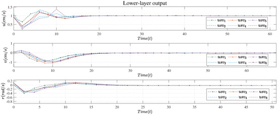
Figure 8.
Lower−layer output.
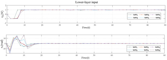
Figure 9.
Lower−layer input.
Figure 5 shows the trajectory in plane coordinates. Scatter points are drawn once every 14 steps. From the trajectory, six USVs could reduce the formation spacing to achieve triangle formation flying with good formation maintenance effect.
Figure 6 shows the output error of the upper-layer control system. It can be seen from the figure that the algorithm could quickly eliminate the upper-level output error. At about step 15, the error in the three degrees of freedom directions was basically zero.
Figure 7 shows the control input of the upper layer, which is the first term of the optimal control sequence obtained by solving the DMPC-based controller every time. From the simulation results, the control input met various constraints, and all six USV converged their speed to the expected value at about 15 steps.
Figure 8 shows the control output of the lower layer. By comparing Figure 8 and Figure 9, it can be seen that the speed response had a certain time delay, but it was within an acceptable range.
Figure 9 shows the control input of the lower layer, which is the first term of the optimal control sequence obtained by solving the MPC-based controller each time.
To verify that the algorithm can achieve the fourth point of the control goal, the following simulation was conducted. In the 17th to 30th steps of the simulation, we manually disrupted communication between USV and USV and used the communication topology in Figure 4b. Similarly, in steps 30 to 45, we manually removed the communication between USV and USV and used the communication topology in Figure 4c. The system was observed to switch the topology immediately to maintain the original formation without the influence of time delay.
The algorithm proposed by Equation (6) is shown in Figure 10, which we call Algorithm 1. Figure 11 does not depict the hypothetical state in the objective function, that is, it does not include the cost of the predicted state deviation from the hypothetical state (item 3 of Equation (6)) or the formation cost (item 4 of Equation (6)); we name this as Algorithm 2. Algorithm 3 was used in [40] and is shown in Figure 12. The difference between Algorithms 2 and 3 is the cost function of upper controller , so for convenience of explanation, we give only the flow of Algorithm 2. It can be seen from a comparison of these three figures that the algorithm with post-verification proposed in this work met the fourth point of the control objectives.
| Algorithm 1: Distributed MPC with post-verification. |
At timet = 0 upper-layer and lower-layer system initialization: At time t 1: Obtain upper-layer system state: 2: Accept neighbor state: 3: Optimize cost function: 4: Obtain: and then pass to the lower-layer system 5: Make up this error in the next time 6: If , then switch topology 7: Obtain lower-layer system state: 8: Optimize cost function: 9: Obtain and apply to system |
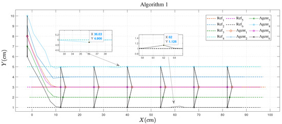
Figure 10.
Output trajectory of Algorithm 1.
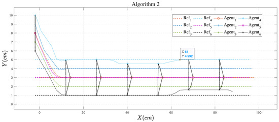
Figure 11.
Output trajectory of Algorithm 2.
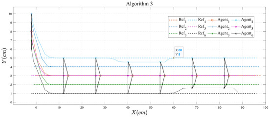
Figure 12.
Output trajectory of Algorithm 3.
| Algorithm 2: Decentralized MPC. |
At timet = 0 upper-layer and lower-layer system initialization: At time t 1: Obtain upper-layer system state: 2: Optimize cost function: 3: Obtain: and then pass to the lower-layer system 4: Obtain lower-layer system state: 5: Optimize cost function: 6: Obtain and apply to system |
Remark 1.
The condition for switching topology is , after switching the trajectory. If the communication is no longer interrupted or wrong, the switched topology is always used. This work assumes that there is always a communication topology that is connected normally, and that there will be no case where a USV cannot accept the formation information from other USVs.
Remark 2.
The stability proof in this work can be found in [26,38].
Figure 10 shows the trajectory evolution using Algorithm 1. We consider that failure occurred in the communication between USV and USV. The failure state condition was satisfied. Consequently, Algorithm 1 switched the current topology (Topology 1 in Figure 4) to an alternative one (Topology 2 in Figure 4). The results show that the method could effectively reduce the formation error. The maximum error was about 0.1 cm and it took about three steps to completely restore the original formation. The same condition was considered in simulations using Algorithms 2 and 3. The results are shown in Figure 11 and Figure 12, respectively. Note that Algorithms 2 and 3 do not adopt the post-verification procedure, and failed to maintain the original USV formation. The difference between Algorithms 2 and 3 lies in the cost function. Specifically, Algorithm 3 employs assumed states of the neighbors in the cost function, which is ignored in Algorithm 2. Simulations revealed that Algorithm 3 had a faster convergence speed compared with Algorithm 2 as failures occurred. Hence, the assumed states of neighbors should be taken into account in the cost function in order to achieve better closed-loop control performance. Similar results were observed when the communication between USV and USV was interrupted. Relevant simulations and analysis are omitted for brevity.
6. Conclusions
In this work, a hierarchical DMPC approach is developed for the formation control of USVs. The upper layer determines the optimal references for the lower layer based on the USV kinematic model and the information received from neighbors. It is shown that the assumed state of the local USV and those of neighbors play important roles in the cost function, which reduces the influence of external disturbances. In addition, a post-verification procedure is adopted which compensates the difference between the assumed states and the actual ones. It is further shown that post-verification can effectively detect the failure state, in which case an alternative communication topology is employed to maintain the USV formation. Simulations reveal the effectiveness of the proposed approach. Our future research will extend the results to multi-agent systems with time delays and unmeasured states.
Author Contributions
T.P. and W.Y.; methodology, W.Y. and T.S.; validation, T.S. and G.H.; formal analysis, G.H. and D.X.; writing, W.Y. and T.S.; review and editing, T.P. and D.X. All authors have read and agreed to the published version of the manuscript.
Funding
This work was supported in part by the National Natural Science Foundation of China under Grants 61903158, 61973140 and 62222307.
Data Availability Statement
The data used to support the findings of this study are available from the corresponding author upon request.
Conflicts of Interest
The authors declare that there are no conflicts of interest regarding the publication of this paper.
References
- Xu, D.; Zhang, W.; Shi, P.; Jiang, B. Model-free cooperative adaptive sliding-mode-constrained-control for multiple linear induction traction systems. IEEE Trans. Cybern. 2019, 50, 4076–4086. [Google Scholar] [CrossRef] [PubMed]
- Shojaei, K. Leader–follower formation control of underactuated autonomous marine surface vehicles with limited torque. Ocean Eng. 2015, 105, 196–205. [Google Scholar] [CrossRef]
- Fu, M.Y.; Wang, D.S.; Wang, C.L. Formation control for water-jet USV based on bio-inspired method. China Ocean Eng. 2018, 32, 117–122. [Google Scholar] [CrossRef]
- Balch, T.; Arkin, R.C. Behavior-based formation control for multirobot teams. IEEE Trans. Robot. Autom. 1998, 14, 926–939. [Google Scholar] [CrossRef]
- Yan, X.; Jiang, D.; Miao, R.; Li, Y. Formation control and obstacle avoidance algorithm of a multi-USV system based on virtual structure and artificial potential field. J. Mar. Sci. Eng. 2021, 9, 161. [Google Scholar] [CrossRef]
- Beard, R.W.; Lawton, J.; Hadaegh, F.Y. A coordination architecture for spacecraft formation control. IEEE Trans. Control Syst. Technol. 2001, 9, 777–790. [Google Scholar] [CrossRef]
- Chen, Q.; Sun, Y.; Zhao, M.; Liu, M. A virtual structure formation guidance strategy for multi-parafoil systems. IEEE Access 2019, 7, 123592–123603. [Google Scholar] [CrossRef]
- Cong, B.L.; Liu, X.D.; Chen, Z. Distributed attitude synchronization of formation flying via consensus-based virtual structure. Acta Astronaut. 2011, 68, 1973–1986. [Google Scholar] [CrossRef]
- Askari, A.; Mortazavi, M.; Talebi, H. UAV formation control via the virtual structure approach. J. Aerosp. Eng. 2015, 28, 04014047. [Google Scholar] [CrossRef]
- Chen, X.; Huang, F.; Zhang, Y.; Chen, Z.; Liu, S.; Nie, Y.; Tang, J.; Zhu, S. A novel virtual-structure formation control design for mobile robots with obstacle avoidance. Appl. Sci. 2020, 10, 5807. [Google Scholar] [CrossRef]
- Sun, X.; Wang, G.; Fan, Y.; Mu, D.; Qiu, B. A formation collision avoidance system for unmanned surface vehicles with leader-follower structure. IEEE Access 2019, 7, 24691–24702. [Google Scholar] [CrossRef]
- Park, B.S.; Yoo, S.J. Connectivity-maintaining and collision-avoiding performance function approach for robust leader–follower formation control of multiple uncertain underactuated surface vessels. Automatica 2021, 127, 109501. [Google Scholar] [CrossRef]
- Yuhan, Z.; Kun, W.; Wei, S.; Zhou, L.; Zhongzhong, Z.; Hao, J.G. Back-stepping Formation Control of Unmanned Surface Vehicles with Input Saturation Based on Adaptive Super-twisting Algorithm. IEEE Access 2022, 10, 114885–114896. [Google Scholar] [CrossRef]
- Liu, X.; Zhang, P.; Du, G. Hybrid adaptive impedance-leader-follower control for multi-arm coordination manipulators. Ind. Robot Int. J. 2016. [Google Scholar] [CrossRef]
- Burlutskiy, N.; Touahmi, Y.; Lee, B.H. Power efficient formation configuration for centralized leader–follower AUVs control. J. Mar. Sci. Technol. 2012, 17, 315–329. [Google Scholar] [CrossRef]
- Zhang, P.; Wang, J. Event-triggered observer-based tracking control for leader-follower multi-agent systems. Kybernetika 2016, 52, 589–606. [Google Scholar] [CrossRef]
- Zhang, S.; Xie, D.; Yan, W. Decentralized event-triggered consensus control strategy for leader–follower networked systems. Phys. A Stat. Mech. Its Appl. 2017, 479, 498–508. [Google Scholar] [CrossRef]
- Hu, J.; Zheng, W.X. Adaptive tracking control of leader–follower systems with unknown dynamics and partial measurements. Automatica 2014, 50, 1416–1423. [Google Scholar] [CrossRef]
- Xie, D.; Yin, X.; Xie, J. Decentralized event-based communication strategy on leader-follower consensus control. Math. Probl. Eng. 2016, 2016, 1048697. [Google Scholar] [CrossRef]
- He, S.; Wang, M.; Dai, S.L.; Luo, F. Leader–follower formation control of USVs with prescribed performance and collision avoidance. IEEE Trans. Ind. Inform. 2018, 15, 572–581. [Google Scholar] [CrossRef]
- Cui, D.; Englot, B.; Cui, R.; Xu, D. Decentralized formation control of multiple autonomous underwater vehicles with input saturation using RISE feedback method. In Proceedings of the OCEANS 2018 MTS/IEEE Charleston, Charleston, SC, USA, 22–25 October 2018; IEEE: New York, NY, USA, 2018; pp. 1–6. [Google Scholar]
- Xu, D.; Zhang, W.; Jiang, B.; Shi, P.; Wang, S. Directed-graph-observer-based model-free cooperative sliding mode control for distributed energy storage systems in DC microgrid. IEEE Trans. Ind. Inform. 2019, 16, 1224–1235. [Google Scholar] [CrossRef]
- Cai, H.; Hu, G. Distributed tracking control of an interconnected leader–follower multiagent system. IEEE Trans. Autom. Control 2017, 62, 3494–3501. [Google Scholar] [CrossRef]
- Hu, J.; Feng, G. Distributed tracking control of leader–follower multi-agent systems under noisy measurement. Automatica 2010, 46, 1382–1387. [Google Scholar] [CrossRef]
- Franzè, G.; Lucia, W.; Tedesco, F. A distributed model predictive control scheme for leader–follower multi-agent systems. Int. J. Control 2018, 91, 369–382. [Google Scholar] [CrossRef]
- Li, X.; Xu, S.; Gao, H.; Cai, H. Distributed tracking of leader-follower multiagent systems subject to disturbed leader’s information. IEEE Access 2020, 8, 227970–227981. [Google Scholar] [CrossRef]
- Hong, Y.; Wang, X.; Jiang, Z.P. Distributed output regulation of leader–follower multi-agent systems. Int. J. Robust Nonlinear Control 2013, 23, 48–66. [Google Scholar] [CrossRef]
- Yan, J.; Yu, Y.; Xu, Y.; Wang, X. A Virtual Point-Oriented Control for Distance-Based Directed Formation and Its Application to Small Fixed-Wing UAVs. Drones 2022, 6, 298. [Google Scholar] [CrossRef]
- Gao, H.; Li, W.; Cai, H. Fully Distributed Robust Formation Flying Control of Drones Swarm Based on Minimal Virtual Leader Information. Drones 2022, 6, 266. [Google Scholar] [CrossRef]
- Oh, S.R.; Sun, J. Path following of underactuated marine surface vessels using line-of-sight based model predictive control. Ocean Eng. 2010, 37, 289–295. [Google Scholar] [CrossRef]
- Liu, L.; Wang, D.; Peng, Z.; Li, T.; Chen, C.P. Cooperative path following ring-networked under-actuated autonomous surface vehicles: Algorithms and experimental results. IEEE Trans. Cybern. 2018, 50, 1519–1529. [Google Scholar] [CrossRef]
- Burger, M.; Pavlov, A.; Borhaug, E.; Pettersen, K.Y. Straight line path following for formations of underactuated surface vessels under influence of constant ocean currents. In Proceedings of the 2009 American Control Conference, St Louis, MO, USA, 10–12 June 2009; IEEE: New York, NY, USA, 2009; pp. 3065–3070. [Google Scholar]
- Gao, Y.; Dai, L.; Xia, Y.; Liu, Y. Distributed model predictive control for consensus of nonlinear second-order multi-agent systems. Int. J. Robust Nonlinear Control 2017, 27, 830–842. [Google Scholar] [CrossRef]
- Li, H.; Shi, Y. Distributed receding horizon control of large-scale nonlinear systems: Handling communication delays and disturbances. Automatica 2014, 50, 1264–1271. [Google Scholar] [CrossRef]
- Morari, M.; Lee, J.H. Model predictive control: Past, present and future. Comput. Chem. Eng. 1999, 23, 667–682. [Google Scholar] [CrossRef]
- Mayne, D.Q.; Rawlings, J.B.; Rao, C.V.; Scokaert, P.O. Constrained model predictive control: Stability and optimality. Automatica 2000, 36, 789–814. [Google Scholar] [CrossRef]
- Wen, J.; Zhao, G.; Huang, S.; Zhao, C. UAV Three-dimensional Formation Keeping Controller Design. In Proceedings of the 2019 Chinese Automation Congress (CAC), Hangzhou, China, 22–24 November 2019; IEEE: New York, NY, USA, 2019; pp. 4603–4608. [Google Scholar]
- Zheng, Y.; Li, S.E.; Li, K.; Borrelli, F.; Hedrick, J.K. Distributed model predictive control for heterogeneous vehicle platoons under unidirectional topologies. IEEE Trans. Control Syst. Technol. 2016, 25, 899–910. [Google Scholar] [CrossRef]
- Jiang, Z.; Jiaming, S.; Zhihao, C.; Yingxun, W.; Kun, W. Distributed coordinated control scheme of UAV swarm based on heterogeneous roles. Chin. J. Aeronaut. 2022, 35, 81–97. [Google Scholar]
- Fan, Z.; Li, H. Two-layer model predictive formation control of unmanned surface vehicle. In Proceedings of the 2017 Chinese Automation Congress (CAC), Jinan, China, 20–22 October 2017; IEEE: New York, NY, USA, 2017; pp. 6002–6007. [Google Scholar]
- Wang, C.N.; Yang, F.C.; Vo, N.T.; Nguyen, V.T.T. Wireless Communications for Data Security: Efficiency Assessment of Cybersecurity Industry—A Promising Application for UAVs. Drones 2022, 6, 363. [Google Scholar] [CrossRef]
- Choi, M.S.; Park, S.; Lee, Y.; Lee, S.R. Ship to ship maritime communication for e-Navigation using WiMAX. Int. J. Multimed. Ubiquitous Eng. 2014, 9, 171–178. [Google Scholar] [CrossRef]


Disclaimer/Publisher’s Note: The statements, opinions and data contained in all publications are solely those of the individual author(s) and contributor(s) and not of MDPI and/or the editor(s). MDPI and/or the editor(s) disclaim responsibility for any injury to people or property resulting from any ideas, methods, instructions or products referred to in the content. |
© 2023 by the authors. Licensee MDPI, Basel, Switzerland. This article is an open access article distributed under the terms and conditions of the Creative Commons Attribution (CC BY) license (https://creativecommons.org/licenses/by/4.0/).