A Comparison of Different Data Fusion Strategies’ Effects on Maize Leaf Area Index Prediction Using Multisource Data from Unmanned Aerial Vehicles (UAVs)

Abstract

The leaf area index (LAI) is an important indicator for crop growth monitoring. This study aims to analyze the effects of different data fusion strategies on the performance of LAI prediction models, using multisource images from unmanned aerial vehicles (UAVs). For this purpose, maize field experiments were conducted to obtain plants with different growth status. LAI and corresponding multispectral (MS) and RGB images were collected at different maize growth stages. Based on these data, different model design scenarios, including single-source image scenarios, pixel-level multisource data fusion scenarios, and feature-level multisource data fusion scenarios, were created. Then, stepwise multiple linear regression (SMLR) was used to design LAI prediction models. The performance of models were compared and the results showed that (i) combining spectral and texture features to predict LAI performs better than using only spectral or texture information; (ii) compared with using single-source images, using a multisource data fusion strategy can improve the performance of the model to predict LAI; and (iii) among the different multisource data fusion strategies, the feature-level data fusion strategy performed better than the pixel-level fusion strategy in the LAI prediction models. Thus, a feature-level data fusion strategy is recommended for the creation of maize LAI prediction models using multisource UAV images.

1. Introduction

The leaf area index (LAI) is a key factor for indicating vegetation growth status. Obtaining LAI and its dynamic change is of great significance for crop health monitoring and yield prediction [1,2]. As an important food and feed crop globally, maize has an important role in ensuring food security [3]. Thus, it is particularly essential to achieve a rapid and nondestructive estimation of maize LAI.

The traditional LAI estimation method is destructive, time-consuming, and labor-intensive, which makes it unsuitable for use in precision agriculture [4]. Remote sensing technology has been demonstrated to be a good tool for crop physiological and biochemical parameter estimation [5,6]. In recent years, with the rapid development of unmanned aerial vehicles (UAVs) and sensor technology, UAV remote sensing technology has been widely used in agriculture. Unlike satellite and manned aerial vehicle remote sensing technology, UAV remote sensing technology can obtain high spatial and temporal resolution images at the field scale at low cost, which is critical for precision agriculture [7,8]. At present, the methods for LAI estimation using UAVs can be classified into two categories: empirical and mechanistic methods. The empirical method uses a data-driven approach to predict LAI of the target area based on the statistical relationship obtained from the collected samples. Although this approach is easy to implement, it needs a large number of samples for model training because of the lack of machinability [9]. The mechanistic method simulates the canopy reflectance spectra by establishing the model of electromagnetic wave radiation transmission in the canopy and taking the physiological and biochemical parameters of vegetation with clear physical explanation as inputs; LAI can be predicted based on its inverse processes [10]. This method has a better mechanistic interpretation and can solve the problem of model generalizability, but due to the large number of input parameters and the complexity of the inversion process, there may also be problems with illness inversion [11,12]. While both methods have their advantages, the empirical method is more commonly used in practice at present.

Using the empirical method to predict LAI based on UAV images, Hasan et al. [13] designed a winter wheat LAI prediction model based on RGB images with partial least squares regression (PLSR). Based on hyperspectral images, Yuan et al. [14] used an artificial neural network (ANN) to build a soybean LAI prediction model. Based on multispectral (MS) images, Shi et al. [15] used support vector regression (SVR) to predict the LAI of red beans and mung beans in tea plantations. Moreover, studies have also documented that the prediction accuracy of crop growth parameters can be improved with the combination of spectral and textural information. Yang et al. [16] designed a new index to estimate rice LAI by coupling spectral and textural features from MS images. Using RGB images, Li et al. [17] estimated rice LAI using the random forest regression (RFR) method based on spectral and textural information. Zhang et al. [18] combined spectral and textural features of UAV MS images to estimate maize LAI. Although the above studies have documented that LAI can be estimated using spectral or texture information from images, they are all based on a single data source. It has been shown that fusing multisource data can combine the advantages of each data source and thus result in better prediction results for vegetation parameters [19,20]. Until recently, it has seldom been applied in the field of UAV LAI prediction.

Multisource image data fusion methods can be classified into three categories: pixel-level fusion, feature-level fusion, and decision-level fusion. Among them, pixel-level fusion is a method that couples the physical quantities of each image element to form a new image with combined characteristics during the preprocessing of remote sensing images [21]. Feature-level fusion is a method that extracts feature information based on different images separately and then fuses the feature information. Decision-level fusion is a method that inverts the target parameters based on different images and then weighs them according to the decision rules [22]. Compared with the decision-level fusion method, the feature-level fusion method and pixel-level fusion method are more commonly used for vegetation parameter inversion using remote sensing images. Among those that used UAV data, a few studies have been conducted with LAI prediction based on feature-level fusion methods. Maimaitijiang et al. [23] used UAV-acquired RGB, MS, and thermal infrared images to extract multimodal information such as spectra, texture, canopy temperature, and structure for soybean yield prediction; Zhu et al. [24] used features extracted from UAV hyperspectral, RGB, thermal infrared, and LiDAR data to investigate the effects of multisource data on the prediction accuracy of maize phenotypic parameters. Liu et al. [25] combined features of UAV MS, RGB, and TIR images to predict maize LAI. The pixel-level fusion method is currently mainly applied in studies using multisource satellite remote sensing images for vegetation parameter inversion [26] and have rarely been reported in UAV remote sensing-related studies. At the same time, there exist no studies that compare different fusion methods for LAI prediction. However, different fusion strategies will definitely have different effects on LAI prediction. Therefore, to more accurately estimate LAI and support precision management, it is important to compare the advantages and disadvantages of different image fusion methods for LAI prediction.

In this study, field experiments, with treatments including different amounts of organic fertilizer, inorganic fertilizer, and straw returned to the field, and different planting densities, were conducted to obtain maize canopies with different LAI values. LAI and corresponding RGB and MS images were collected at different stages of maize growth. Based on these data, this study focuses on the recommended optimal strategy for LAI prediction. The purposes of this study were (i) to analyze whether both the pixel-level fusion method and feature-level fusion method could obtain a better prediction accuracy for LAI than the single-source data method using UAV data, and (ii) to recommend a better fusion strategy for LAI prediction by comparing the pixel-level fusion method and feature-level fusion method.

2. Materials and Methods

2.1. Field Experiment

The eastern part of the Inner Mongolia Autonomous Region is an important black soil area in China and an important area for maize production. Our experiment was conducted in 2022 at Dahewan Farm (123°1′33″ E, 47°54′2″ N) in Zalantun city. The area belongs to the temperate semi-humid continental monsoon climate zone with fertile soil and sufficient sunshine. The maize cultivar “Huaqing 6” was used in the experiment with different field treatment trials, including different amounts of inorganic fertilizer, organic fertilizer, and straw returned to the field, and different planting densities (Figure 1). The inorganic fertilizer treatment included four nitrogen application levels (N₁: 150 kg hm⁻², N₂: 180 kg hm⁻², N₃: 210 kg hm⁻², and N₄: 240 kg hm⁻²), three phosphate (P₂O₅) application levels (P₁: 60 kg hm⁻², P₂: 75 kg hm⁻², and P₃: 90 kg hm⁻²) and three potash (K₂O) fertilizer levels (K₁: 75 kg hm⁻², K₂: 90 kg hm⁻², and K₃: 105 kg hm⁻²); the organic fertilizer treatment had five levels (O₁: 0 kg hm⁻², O₂: 22,500 kg hm⁻², O₃: 37,500 kg hm⁻², O₄: 45,000 kg hm⁻², and O₅: 52,500 kg hm⁻²); the treatment with straw returned to the field had five levels (R₁: 0 kg hm⁻², R₂: 3000 kg hm⁻², R₃: 4500 kg hm⁻², R₄: 6000 kg hm⁻² and R₅: 7500 kg hm⁻²); and the treatment with varying planting density had five levels (D₁: 50,000 plants hm⁻², D₂: 55,000 plants hm⁻², D₃: 60,000 plants hm⁻², D₄: 62,000 plants hm⁻², and D₅: 64,000 plants hm⁻²). All treatments were performed with two replications. In addition, two zero-fertilizer plots (T₀: 0 kg hm⁻²) and two plots with a stable compound fertilizer (T₁: 750 kg hm⁻² of stable compound fertilizer with an N-P₂O₅-K₂O ratio of 26-10-12) were also included in the experiment. The organic fertilizer, straw returned to the field, and varying planting density treatments received a stable compound fertilizer at an N-P₂O₅-K₂O ratio of 26-10-12 at 750 kg hm⁻². The plot size is about 30 m². Except for the differences in treatments mentioned above, all other field management measures were the same.

2.2. Data Acquisition and Processing

Field campaigns were conducted during the V4 and V9 growth stages of maize to obtain UAV images and perform field LAI measurements. These two growth stages are critical for maize water and fertilizer management.

2.2.1. UAV Data Acquisition

A self-designed tail-seat vertical takeoff and landing fixed-wing UAV equipped with an Altum MS camera (MicaSense, Washington, DC, USA) and a Sony RX1RII digital camera (Sony, Tokyo, Japan) was used to acquire maize RGB images and MS images, respectively (Figure 2). Compared to fixed-wing UAVs and rotary-wing UAVs, the vertical takeoff and landing fixed-wing UAV combines the advantages of low requirements for takeoff and landing of rotary-wing UAVs and the long working time and fast speed of fixed UAVs. The central wavelength and bandwidth of the Altum camera are shown in

Table 1. Information for the visible to near-infrared bands of the Altum MS camera.

Band Name	Central Wavelength (nm)	Bandwidth (nm)
Blue	475	20
Green	560	20
Red	668	10
Red edge	717	10
Near-infrared	840	40

. The image size is 2064 × 1544 pixels. Sony RX1RII has an image size of 7952 × 5340 pixels. In order to ensure the reliability of the data, the flight time was from 10:00 to 12:00 on a sunny and windless day. The flight height was 150 m for the acquisition of both types of images. For the MS camera, a 75% forward overlap and 75% side overlap were set, and for the RGB camera, the forward overlap was set to 72%, and the side overlap was set to 75%. The spatial resolution of the acquired RGB images was 2.3 cm, and the spatial resolution of the MS images was 8.8 cm. For MS images, digital number (DN) values were converted to reflection values with the help of a white panel image taken before UAV take-off. Meanwhile, 46 ground control points (GCPs) were uniformly distributed in the field, and the longitude and latitude information of GCPS was measured based on the GEO7X (Trimble, Sunnyvale, CA, USA) global positioning system (GPS) with a centimeter-level error.

For UAV image processing, first, RGB and MS images were mosaicked using the Pix4Dmapper (Pix4D, Lausanne, Switzerland). Second, ArcGIS (Esri, Redlands, CA, USA) was used to perform geometrical correction of the mosaicked RGB images using GCPs. Third, the mosaicked MS image was geo-corrected based on the corrected RGB image.

2.2.2. Field-Measured Data

After the UAV was flown, areas with uniform maize growth were selected as representative sample points in each plot, and their locations were measured using the abovementioned GEO 7X in NRTK mode. Then, the LAI 2200 Plant Canopy Analyzer (LI-COR Inc., Lincoln, NE, USA) was used to measure maize LAI according to the manual of the instrument. During this process, the distance between two adjacent rows was divided into four equal parts, and LAI was measured at each position and averaged [27].

2.3. Data Analysis

To analyze the effects of different modeling strategies on LAI prediction, this study included different scenarios based on RGB and MS image use. For each scenario, stepwise multiple linear regression (SMLR) was used to create the LAI prediction model. The results were compared and analyzed to show the advantages and disadvantages of each modeling strategy. The details of modeling are shown in Figure 3.

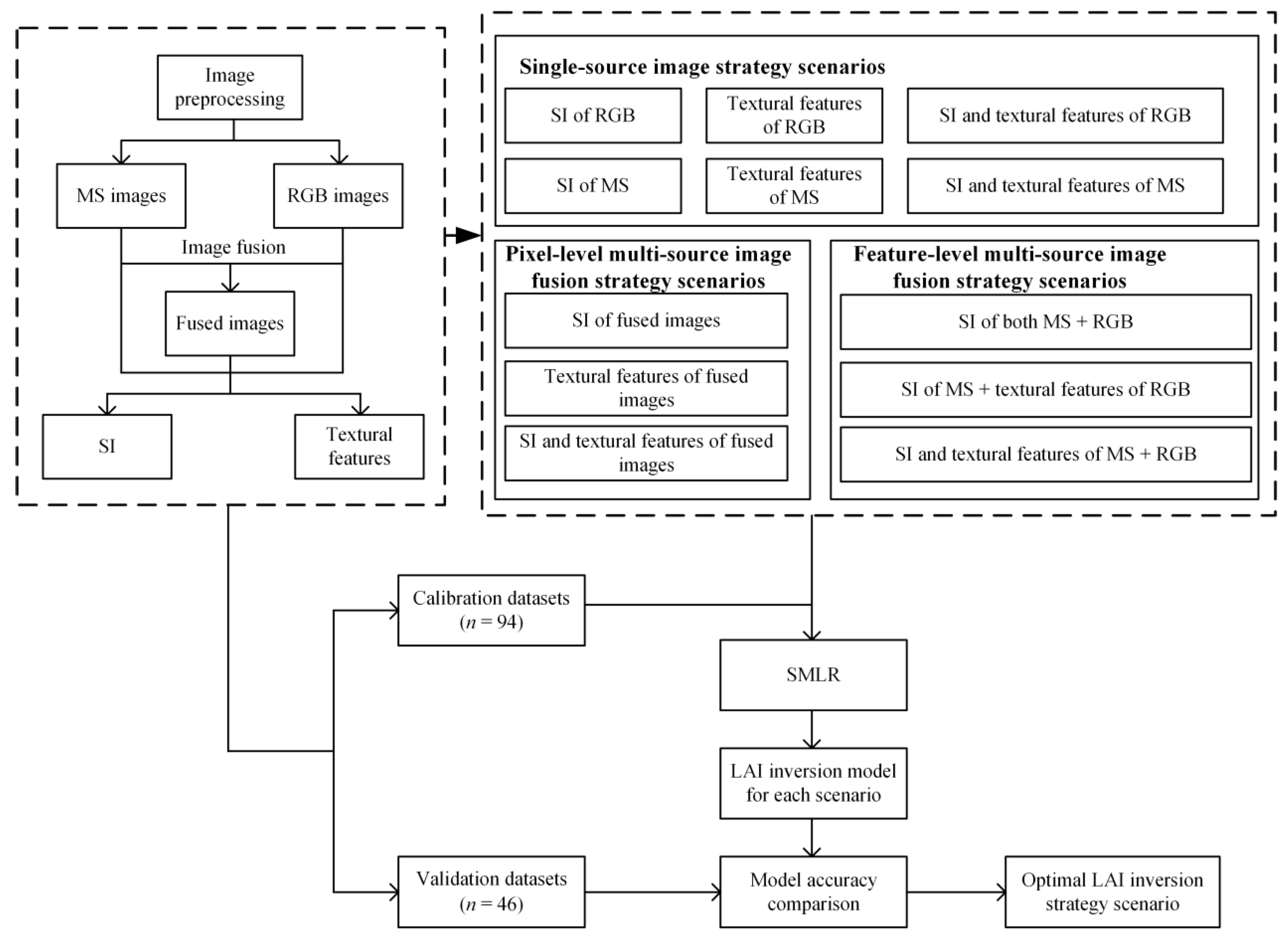
2.3.1. Different Prediction Strategy Scenarios

To compare the effects of different prediction strategies on LAI prediction, scenarios were designed and can be classified into three categories: (1) Single-source data strategy scenarios. This category included six scenarios: (i) spectral information (SI) of MS; (ii) SI of RGB; (iii) textural features of RGB; (iv) textural features of MS; (v) SI and textural features of MS; and (vi) SI and textural features of RGB. (2) Pixel-level multisource data fusion strategy scenarios. This category included three scenarios: (i) textural features of pixel-level fused images; (ii) SI of pixel-level fused images; and (iii) SI and textural features of pixel-level fused images. (3) Feature-level multisource data fusion strategy scenarios. This category included three scenarios: (i) SI of both MS + RGB; (ii) SI of MS + textural features of RGB; and (iii) SI and textural features of both MS + RGB.

Notably, the pixel-level fused image was obtained by the fusion method proposed by Selva et al. [28]. According to their study, the acquired RGB and MS images were fused according to Equations (1)–(5).

$${\widehat{hs}}_n={hs}_{nexp}+g_n·(X_n-{\tilde{X}}_{nexp})$$

(1)

$$g_n=\frac{cov({hs}_{nexp},{\tilde{X}}_{nexp})}{var\left({\tilde{X}}_{nexp}\right)}$$

(2)

$$X_n=\sum _{m=1}^M{w}_{nm}·{HS}_m+b_n$$

(3)

$$\overline{m}=\underset{m}{\arg \max \mathit{corr}}({hs}_{nexp},{\widetilde{HS}}_{mexp})$$

(4)

$$w_{nm}=\left\{\begin{array}{c}1,\hspace{1em}ifm=\overline{m}\\ 0,\hspace{1em}otherwise\end{array}\right.$$

(5)

where ${\widehat{hs}}_n$ indicates the nth band of the fused high spatial resolution image; ${hs}_{nexp}$ indicates the nth band of the interpolated MS image at high spatial resolution; $g_n$ indicates a gain factor; ${\tilde{X}}_{nexp}$ indicates the nth band of ${\tilde{X}}_n$ interpolated at high spatial resolution; ${\tilde{X}}_n$ indicates the nth band of $X_n$ downsampled to a low spatial resolution; ${HS}_m$ indicates the mth band of the original RGB image; ${\widetilde{HS}}_{mexp}$ indicates the mth band of the RGB image downsampled to a low spatial resolution, and then interpolated to a high spatial resolution; $\overline{m}$ indicates the band in ${\widetilde{HS}}_{mexp}$ which has the best relationship with ${hs}_{nexp}$; $w_{nm}$ and $b_n$ indicate the weight and the constant, respectively. $b_n$ was set to 0 according to Selva et al. [28].

2.3.2. Image Feature Extraction

A spectral index effectively indicates the growth of vegetation by combining specific spectral bands to reduce the effects of background factors and enhance vegetation information [29]. UAV images are also rich in texture information which can indicate vegetation growth status apart from spectral information [30]. Therefore, in this study, first, for each type of image (RGB, MS, and fused images), the mean value of all pixels within a circular area (a radius equal to the row spacing) centered at the measured sampling point were calculated to correspond to the LAI value at that point. Then, commonly used spectral indices of MS/fused images (

Table 2. Spectral indices used in this study for MS and fused images.

SI	Full Name	Formula	Source
RVI	Ratio Vegetation Index	$NIR/R$	[32]
GRVI	Green Ratio Vegetation Index	$NIR/G-1$	[33]
DVI	Difference Environmental Vegetation Index	$NIR-R$	[34]
RESR	Red-Edge Simple Ratio	$RE/R$	[35]
NDVI	Normalized Difference Vegetation Index	$(NIR-R)/(NIR+R)$	[36]
NDRE	Normalized Difference Red Edge Index	$(NIR-RE)/(NIR+RE)$	[37]
EVI	Enhanced Vegetation Index	$2.5(NIR-R)/(NIR+6R-7.5B+1)$	[38]
MSAVI	Modified Soil-Adjusted Vegetation Index	$(2NIR+1-sqrt({(2NIR+1)}^2-8(NIR-R)))/2$	[39]
OSAVI	Optimized Soil-Adjusted Vegetation Index	$1.16(NIR-R)/(NIR+R+0.16)$	[40]
GNDVI	Green Normalized Difference Vegetation Index	$(NIR-G)/(NIR+G)$	[41]
TVI	Triangular Vegetation Index	$60(NIR-G)-100(R-G)$	[42]
SAVI	Soil-Adjusted Vegetation Index	$1.5(NIR-R)/(NIR+R+0.5)$	[43]
RENDVI	Red Edge Normalized Difference Vegetation Index	$(RE-R)/(RE+R)$	[44]
MCARI	Modified Chlorophyll Absorption Ratio Index	$((RE-R)-0.2(RE-G))(RE/R)$	[45]
TCARI	Transformed Chlorophyll Absorption in Reflectance Index	$3((RE-R)-0.2(RE-G)(RE/R))$	[46]
TCARI/OSAVI	Combined Spectral Index	$TCARI/OSAVI$	[47]
VARI	Visible Atmospherically Resistant Index	$(G-R)/(G+R-B)$	[48]
RDVI	Re-normalized Difference Vegetation Index	$(NIR-R)/sqrt(NIR+R)$	[49]
MSR	Modified Simple Ratio	$(NIR/R-1)/sqrt(NIR/R+1)$	[50]
NGI	Normalized Green Index	$G/(NIR+G+RE)$	[51]

B, G, R, RE, and NIR indicate the bands of the MS and fused image.

) and RGB images (

Table 3. Spectral indices used in this study for RGB images.

SI	Full Name	Formula	Source
GBRI	Green–Blue Ratio Index	$g/b$	[13]
GRRI	Green–Red Ratio Index	$g/r$	[52]
BRRI	Blue–Red Ratio Index	$b/r$	[53]
ExG	Excess Green	$2g-r-b$	[54]
ExR	Excess Red	$1.4r-g$	[55]
ExGR	Excess Green Minus Excess Red	$E\mathrm{xG}-E\mathrm{xR}$	[56]
NGRDI	Normalized Green–Red Difference Index	$(g-r)/(g+r)$	[57]
RGBVI	Red–Green–Blue Vegetation Index	$(g^2-br)/(g^2+br)$	[58]
CIVE	Color Index of Vegetation	$0.441r-0.811g+0.385b+18.78745$	[59]
MExG	Modified Excess Green	$1.262g-0.884r-0.311b$	[60]
GLA	Green Leaf Algorithm	$(2g-r-b)/(2g+r+b)$	[61]
VARI	Visible Atmospherically Resistant Index	$(g-r)/(g+r-b)$	[62]
NGBDI	Normalized Green–Blue Difference Index	$(g-b)/(g+b)$	[63]

r, g, and b indicate the normalized bands of the RGB image; r = R/(R + G + B), g = G/(R + G + B), and b = B/(R + G + B).

) were calculated. Notably, for RGB image data, it has been shown that the normalized visible band has a better estimation capability than the original visible band [31]. Thus, the bands were normalized before being used for the calculation of the spectral indices of RGB images. In addition, the textural features of the three types of images were also extracted, including mean (mea), variance (var), homogeneity (hom), contrast (con), dissimilarity (dis), entropy (ent), second moment (sec), and correlation (cor). During these processes, the gray-level co-occurrence matrix (GLCM) method was used to calculate the textural features of each band using ENVI 5.6 (Exelis VIS, Boulder, CO, USA).

2.3.3. Model Design for Each Scenario

To analyze the effects of different strategies for designing an LAI prediction model and clearly show which variables are used in the model, the study used SMLR. SMLR is a linear regression model with multiple independent variables [64], which reduces the covariance problem by introducing variables into the model one by one; each time a variable is introduced, the variables already selected are tested one by one to ensure that only significant variables are included in the regression equation. Before model design, the collected data were divided into calibration datasets (n = 94) and validation datasets (n = 46) at a ratio of 2:1. The calibration dataset was used to design the LAI prediction model, and validate the model based on the validation dataset. The adjusted determination coefficient (R²_adj), root mean square error (RMSE_cal), and Akaike information criterion (AIC) during model calibration, and the determination coefficient (R²) and root mean square error (RMSE_val) during model validation were used to evaluate model performance. Notably, all scenarios were based on the same calibration and validation datasets during the design of the LAI prediction model. In this study, SPSS (IBM, New York, USA) was used to implement SMLR modeling. Additionally, before designing the multiple linear models, the conditions were examined to make sure they satisfy the assumptions, such as linearity, equal variance, independence, and normality.

3. Results and Analysis

3.1. LAI in the Field

The statistical analysis results of LAI obtained in the field experiment are shown in

Table 4. Statistical analysis results of LAI in the maize field experiment.

Growth Stage	Number of Samples	Min. Value	Max. Value	Average Value	Standard Deviation	Variance	Coefficient of Variation (%)
V4 stage	70	0.37	2.20	0.83	0.34	0.11	40.96
V9 stage	70	1.61	3.19	2.31	0.34	0.12	14.72

. The data show a large variation for both growth stages, indicating that different maize canopy LAI values were obtained in this study through the different experimental treatments. Overall, the LAI values ranged from 0.37 to 3.19, covering a wide range during these two maize growth stages, which are critical periods for fertilizer management; thus, the results can support the comparative analysis of different LAI prediction strategies. We should note that, as the aim of this study is to compare the performance of different strategies for LAI prediction model designing, the LAI values for each treatment are not shown herein for clarity.

3.2. Comparison of the Original Image and Pixel-Level Fused Image

The RGB and MS images were fused in this study, and the images before and after fusion are shown in Figure 4. The fused image not only has the textural information from the RGB image but also has the spectral information from the MS image. Overall, a good pixel-level fused image was obtained, which ensures accurate assessments based on the pixel-level fused images in this study.

3.3. Results of LAI Inversion for the Single-Source Image Strategy Scenarios

The results of the LAI prediction models designed using a single-source data strategy are shown in

Table 5. LAI prediction results based on single-source image strategy scenarios.

Strategy	Model	Calibration			Validation
		R2adj	RMSEcal	AIC	R2	RMSEval
SI of MS	$y=13.55\ast NDRE-6.293\ast NDVI+0.491$	0.838	0.315	−211.26	0.897	0.283
Textural features of MS	$\begin{array}{l}y=0.154\ast nir\_mea-0.225\ast re\_mea\\ +0.184\ast b\_mea+0.743\end{array}$	0.817	0.332	−198.62	0.881	0.303
SI and textural features of MS	$\begin{array}{l}y=14.944\ast NDRE-6.424\ast NDVI\\ +4.603\ast re\_ent-0.028\ast nir\_con-9.202\end{array}$	0.859	0.291	−221.89	0.899	0.273
SI of RGB	$\begin{array}{l}y=-66.07\ast BRRI-137.778\ast E\mathrm{xR}\\ -39.775\ast GBRI+123.845\end{array}$	0.819	0.332	−199.42	0.875	0.316
Textural features of RGB	$\begin{array}{l}y=-0.348\ast R\_mea+0.335\ast B\_mea\\ +11.235\ast G\_\sec +2.698\end{array}$	0.826	0.325	−203.29	0.902	0.289
SI and textural features of RGB	$\begin{array}{l}y=13.619\ast BRRI-0.093\ast B\_mea\\ +12.116\ast G\_\sec -8.27\end{array}$	0.833	0.319	−207.01	0.903	0.283

R, G, and B indicate the Red, Green, and Blue bands of the RGB image; b, re, and nir indicate the blue, red-edge, and near-infrared bands of the MS image, respectively; B_*, G_*, and R_* indicate the * textural values of the bands in the RGB image, respectively; and b_*, re_*, and nir_* indicate the * textural values of the bands in the MS image, respectively.

. In summary, regardless of whether it was based on MS images or RGB images, the strategies that used both SI and textural features to design the model performed better than the strategies that used only SI or textural features. In addition, the LAI prediction model designed with SI and textural features of MS images had the best performance, which is also shown in Figure 5. We should note that, for each section, we only gave figures for best results for concision.

For the MS image, when the designed LAI prediction model used both SI and textural features, two spectral indices (NDVI and NDRE) and two textural features (re_ent and nir_con) were selected as independent variables in the model. While the R²_adj, RMSE_cal, and AIC of the model were 0.859, 0.291, and −221.89 during calibration, the validation values of R² and RMSE_val were 0.899 and 0.273. Considering the accuracy of the models, the SI model was followed, with NDVI and NDRE selected as independent variables. The R²_adj, RMSE_cal, and AIC of the model were 0.838, 0.315, and −211.26 during calibration, while the R² and RMSE_val were 0.897 and 0.283 during validation. The LAI model designed with only textural features performed the worst, with nir_mea, re_mea, and b_mea selected as independent variables. It had an R²_adj of 0.817, RMSE_cal of 0.332, and AIC of −198.62 during calibration, and an R² of 0.881 and RMSE_val of 0.303 during validation.

For the RGB image, when the designed LAI prediction model used both SI and textural features, one spectral index (BRRI) and two textural features (B_mea and G_sec) were selected as independent variables in the model. While the R²_adj, RMSE_cal and AIC of the model were 0.833, 0.319, and −207.01 during calibration, the validation values of R² and RMSE_val were 0.903 and 0.283 (Table 5). Different from the MS image, the prediction model designed with only textural features performed better than the model designed with only SI. This may be because the RGB image has a higher spatial resolution and lower spectral information than the MS image, making the textual features of the image more important than SI for LAI prediction. For the model designed with only textural features, R_mea, B_mea, and G_sec were selected as the independent variables. The calibration R²_adj, RMSE_cal, and AIC of the model were 0.826, 0.325, and −203.29, while the validation R² and RMSE_val were 0.902 and 0.289. For the LAI prediction model with SI, BRRI, ExR and GBRI were selected as the independent variables. The R²_adj, RMSE_cal, and AIC were 0.819, 0.332, and −199.42 during calibration, and the R² and RMSE_val were 0.875 and 0.316 during validation.

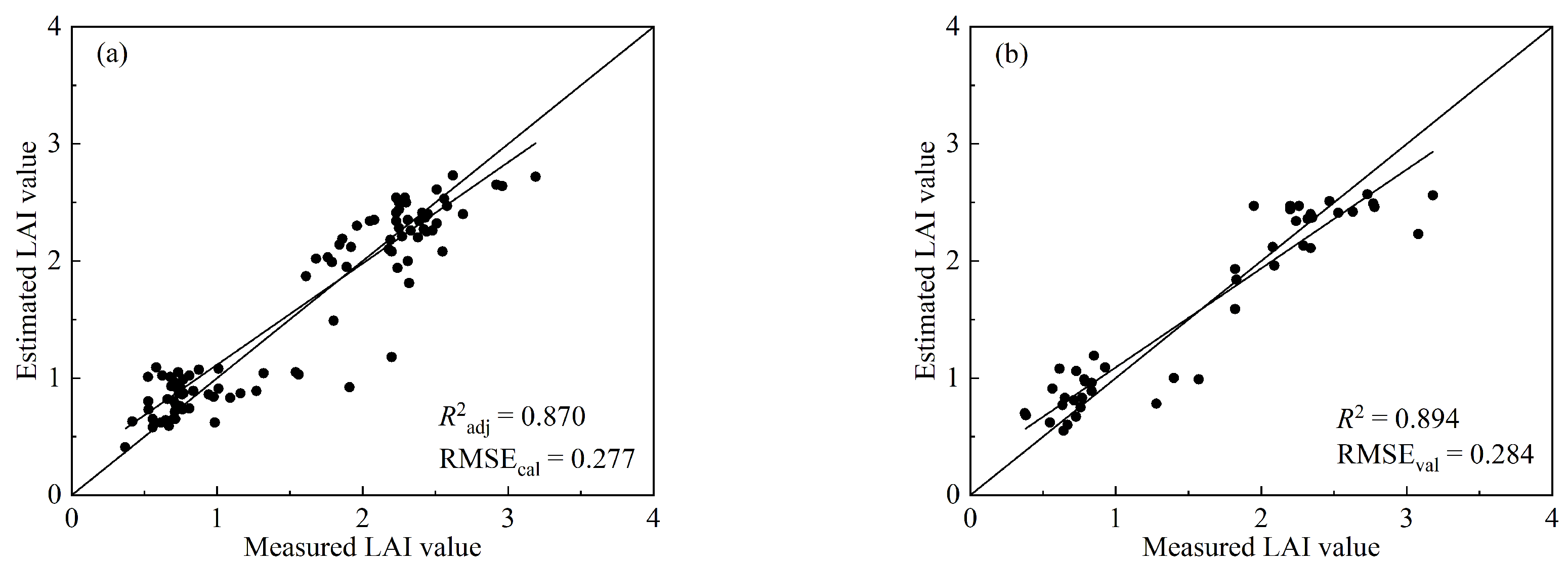
3.4. Results of LAI Inversion for Pixel-Level Data Fusion Strategy Scenarios

The results of the LAI prediction models designed using the pixel-level data fusion scenarios are shown in

Table 6. LAI prediction results based on pixel-level data fusion strategy scenarios.

Strategy	Model	Calibration			Validation
		R2adj	RMSEcal	AIC	R2	RMSEval
SI of fused image	$y=13.463\ast NDRE-6.228\ast NDVI+0.483$	0.837	0.316	−210.65	0.896	0.285
Textural features of fused image	$\begin{array}{l}y=0.093\ast nir\_mea+0.232\ast b\_mea+\\ 4.07\ast g\_cor-0.312\ast g\_mea-1.169\end{array}$	0.861	0.288	−223.82	0.898	0.280
SI + textural features of fused image	$\begin{array}{l}y=8.399\ast NDRE-3.523\ast NDVI\\ +2.925\ast g\_cor-1.564\ast r\_\mathrm{var}\\ +2.089\ast b\_\mathrm{var}-0.757\end{array}$	0.870	0.277	−229.20	0.894	0.284

b, g, r, and nir indicate the blue, green, red, and near-infrared bands; b_*, g_*, r_*, and nir_* indicate the * textural values of the bands in the fused image, respectively.

. The model designed with both SI and textural features had the best accuracy, with two spectral indices (NDRE and NDVI) and three textural features (g_cor, r_var, and b_var) selected as independent variables. It had calibration R²_adj of 0.870, RMSE_cal of 0.277, and AIC of −229.20, and validation R² of 0.894 and RMSE_val of 0.284 (Figure 6). The performance of the model designed using only textural features followed, with nir_mea, b_mea, g_cor, and g_mea selected as the independent variables. It had calibration R²_adj of 0.861, RMSE_cal of 0.288, and AIC of −223.82, and validation R² of 0.898 and RMSE_val of 0.280. The LAI prediction model designed with only SI had the worst performance. For this model, NDVI and NDRE were selected as the independent variables, with calibration R²_adj of 0.837, RMSE_cal of 0.316, and AIC of −210.65, and validation R² of 0.896 and RMSE_val of 0.285.

3.5. Results of LAI Inversion for Feature-Level Data Fusion Strategy Scenarios

The results of the LAI prediction models designed using the feature-level data fusion scenarios are shown in

Table 7. LAI prediction results based on feature-level data fusion strategy scenarios.

Strategy	Fitting Model	Calibration			Validation
		R2adj	RMSEcal	AIC	R2	RMSEval
SI of MS + RGB	$\begin{array}{l}y=10.08\ast NDRE-4.389\ast NDVI+\\ 3.734\ast BRRI-2.369\end{array}$	0.844	0.308	−213.44	0.902	0.277
SI of MS + textural features of RGB	$\begin{array}{l}y=12.793\ast NDRE-5.693\ast NDVI\\ +3.53\ast G\_cor-1.839\end{array}$	0.849	0.303	−216.46	0.890	0.292
SI and textural features of MS + RGB	$\begin{array}{l}y=11.61\ast NDRE-3.485\ast NDVI+\\ 5.849\ast re\_ent+16.185\ast G\_\sec -\\ 0.074\ast R\_mea-0.036\ast nir\_con\\ -3.013\ast GBRI-8.056\end{array}$	0.883	0.261	−236.61	0.905	0.263

R and G indicate the red and green bands of the RGB image, respectively; re and nir indicate the red-edge and near-infrared bands of the MS image, respectively; G_* and R_* indicate the * textural values of the bands in the RGB image, respectively; re_*and nir_* indicate the * textural values of the bands in the MS image.

. The LAI prediction model designed using SI and textural features of both MS + RGB images had the best accuracy, with two spectral indices (NDRE and NDVI) and two textural features (re_ent and nir_con) from the MS image, and one spectral index (GBRI) and two textural features (R_mea and G_sec) from the RGB image selected as the independent variables. It had calibration R²_adj of 0.883, RMSE_cal of 0.261, and AIC of −236.61, and validation R² of 0.905 and RMSE_val of 0.263 (Figure 7). The performance of the LAI prediction model created with the SI of the MS image and textural features of the RGB image followed. For this model, two spectral indices of the MS image (NDRE and NDVI) and one textural feature (G_cor) of the RGB image were selected as the independent variables, with calibration R²_adj of 0.849, RMSE_cal of 0.303, and AIC of −216.46, and validation R² of 0.890 and RMSE_val of 0.292. For the LAI prediction model with the SI of both the MS and RGB images, two spectral indices (NDRE and NDVI) and one spectral index (BRRI) of the RGB image were selected as the independent variables; the R²_adj, RMSE_cal, and AIC were 0.844, 0.308, and −213.44 during calibration, and the R² and RMSE_val were 0.902 and 0.277 during validation.

4. Discussion

4.1. Comparison with Previous Studies

In this study, UAV RGB, MS, and fused images were used to make single-source data, pixel-level fusion data, and feature-level fusion data scenarios for creating LAI prediction models based on the SMLR method. The R²_adj of models varied from 0.817 to 0.883 and the RMSE varied from 0.261 to 0.332 during calibration, while the R² varied from 0.875 to 0.905 and the RMSE varied from 0.263 to 0.316 during validation. Considering previous studies of LAI prediction, Zhang et al. [18] designed a maize LAI estimation model with the SVR method using spectral and textural features of UAV MS images, and the model had R² values of 0.877 during validation. Combining spectral and textural indices extracted from UAV MS images, Sun et al. [65] used the SVR method to design a maize LAI prediction model, with an R² of 0.806 during calibration and an R² of 0.813 during validation. Liu et al. [25] combined features extracted from UAV MS, RGB, and TIR images to predict maize LAI with the PLSR method; the R² of calibration was 0.78 and the R² of validation was 0.70. Compared with the above studies, the results of the prediction models created in this study under different scenarios are within a reasonable range.

Moreover, due to limitations created by time and weather conditions, the timeframe for crop growth status monitoring is short. Thus, for large areas, an efficient means for UAV image acquisition is urgently needed. In this study, we adopted a self-designed tail-seat vertical takeoff and landing fixed-wing UAV platform to acquire UAV images. As mentioned before, the UAV platform uses the rotor-wing mode to takeoff and land and the fixed-wing mode to acquire data, which has the advantage of flexibility without the need for an aircraft runway and can also acquire data more efficiently than rotor-wing UAV platforms. The results of this study support the application of our designed vertical takeoff and landing fixed-wing UAV for crop status monitoring.

4.2. Optimal LAI Prediction Strategy

In this study, different LAI prediction strategies were compared, including single-source image-based, pixel-level multisource data fusion, and feature-level multisource data fusion strategies. The results indicate that (1) compared with using only SI or textural features, the LAI prediction model created with a combination of SI and textural features had the best performance. The results validate the accuracy of previous relevant studies [16,66]. This may be because SI always has saturation problems at medium to high LAI levels [67], while textural features can describe the spatial geometric information of plants. Combining these data sources with spectral information could solve the saturation problem to a certain extent and improve the LAI prediction accuracy. (2) Compared with LAI prediction models created using single-source images, the results of LAI prediction models created with multisource image fusion strategies performed better. This is probably because data fusion can combine the advantages of high spatial resolution in RGB images and multiple bands containing red-edge, and near-infrared bands in MS images, which is critical for LAI prediction. Furthermore, this study documented that the LAI prediction models created with the pixel-level fusion strategy performed better than the models created with single-source data, which have rarely been reported for crop parameter prediction using UAV images in existing studies. (3) For different data fusion strategies, the LAI prediction model created with the feature-level data fusion strategy performed better than the model created with the pixel-level data fusion strategy. This may be because LAI prediction models based on the pixel-level fusion strategy have flaws caused by spatial registration errors between images and errors created by the method used for pixel-level fusion. LAI prediction models created with the feature-level fusion strategy directly extract features from different images separately and then combine them using statistical methods, reducing the errors during data preprocessing. In summary, from the above analysis, a feature-level data fusion method is recommended for creating an LAI prediction model when multisource image data are available.

4.3. Limitations and Future Work

The data measured in this study are limited to the topdressing management stage of maize (V4–V9), and the data in the later growth stage were not collected, which limited the ability of the model developed in this study to be applied to other growth stages of maize. Therefore, to apply the best LAI prediction model created in this study in different scenarios, it is necessary to collect a large dataset from different locations, years, and growth stages to further optimize the model in the future. Moreover, the aim of this study is to determine the best strategy for using multisource UAV images to predict LAI, so only SMLR was used because it is simple and can clearly analyze the independent variables used in the model. For the future, it is possible to use more complex methods, such as deep learning methods, to predict LAI based on feature-level fusion strategies.

5. Conclusions

In this study, different treatments (different amounts of organic fertilizer, inorganic fertilizer, and straw returned to the field, and different planting densities) were used to obtain maize plants with different growth statuses, and field LAI data and corresponding UAV MS and RGB images were measured at different growth stages. Single-source image-based scenarios, pixel-level multisource data fusion scenarios, and feature-level multisource data scenarios were designed based on these data, and LAI prediction models were created under different scenarios, leading to a recommendation of the optimal LAI prediction strategy. The results showed that (1) combining spectral and texture features to predict LAI performed better than using only spectral or texture information; (2) compared with using a single-source image, using a multisource data fusion strategy can increase the accuracy of the model in predicting LAI; and (3) among different multisource data fusion strategies, the feature-level data fusion strategy performed better than the pixel-level fusion strategy in the LAI prediction model. Among all the LAI prediction models, the prediction model that used SI and textural features of both MS + RGB had the highest accuracy, with calibration R²_adj of 0.883, RMSE_cal of 0.261, and AIC of −236.61, and validation R² of 0.905 and RMSE_val of 0.263. The feature-level multisource data fusion strategy is recommended as the optimal strategy for creating an LAI prediction model in this study, providing a reference for people to more accurately estimate crop LAI in the field.

References

1. Luo, L.L.; Chang, Q.R.; Gao, Y.F.; Jiang, D.Y.; Li, F.L. Combining Different Transformations of Ground Hyperspectral Data with Unmanned Aerial Vehicle (UAV) Images for Anthocyanin Estimation in Tree Peony Leaves. Remote Sens. 2022, 14, 2271. [Google Scholar] [CrossRef]
2. Collins, W. Remote sensing of crop type and maturity. Photogramm. Eng. Remote Sens. 1978, 44, 42–55. [Google Scholar]
3. Palacios-Rojas, N.; McCulley, L.; Kaeppler, M.; Titcomb, T.J.; Gunaratna, N.S.; Lopez-Ridaura, S.; Tanumihardjo, S.A. Mining maize diversity and improving its nutritional aspects within agro-food systems. Compr. Rev. Food Sci. Food Saf. 2020, 19, 1809–1834. [Google Scholar] [CrossRef]
4. Yan, G.J.; Hu, R.H.; Luo, J.H.; Weiss, M.; Jiang, H.L.; Mu, X.H.; Xie, D.H.; Zhang, W.M. Review of indirect optical measurements of leaf area index: Recent advances, challenges, and perspectives. Agric. For. Meteorol. 2019, 265, 390–411. [Google Scholar] [CrossRef]
5. Yue, J.B.; Feng, H.K.; Yang, G.J.; Li, Z.H. A Comparison of Regression Techniques for Estimation of Above-Ground Winter Wheat Biomass Using Near- Surface Spectroscopy. Remote Sens. 2018, 10, 66. [Google Scholar] [CrossRef]
6. Fu, Y.Y.; Yang, G.J.; Li, Z.H.; Song, X.Y.; Li, Z.H.; Xu, X.G.; Wang, P.; Zhao, C.J. Winter Wheat Nitrogen Status Estimation Using UAV-Based RGB Imagery and Gaussian Processes Regression. Remote Sens. 2020, 12, 3778. [Google Scholar] [CrossRef]
7. Sumesh, K.C.; Ninsawat, S.; Som-ard, J. Integration of RGB-based vegetation index, crop surface model and object-based image analysis approach for sugarcane yield estimation using unmanned aerial vehicle. Comput. Electron. Agric. 2021, 180, 105903. [Google Scholar] [CrossRef]
8. Han, L.; Yang, G.J.; Dai, H.Y.; Xu, B.; Yang, H.; Feng, H.K.; Li, Z.H.; Yang, X.D. Modeling maize above-ground biomass based on machine learning approaches using UAV remote-sensing data. Plant Methods 2019, 15, 10. [Google Scholar] [CrossRef] [PubMed]
9. Ma, X.; Chen, P.F.; Jin, X.L. Predicting Wheat Leaf Nitrogen Content by Combining Deep Multitask Learning and a Mechanistic Model Using UAV Hyperspectral Images. Remote Sens. 2022, 14, 6334. [Google Scholar] [CrossRef]
10. Li, Z.H.; Jin, X.L.; Wang, J.H.; Yang, G.J.; Nie, C.W.; Xu, X.G.; Feng, H.K. Estimating winter wheat (Triticum aestivum) LAI and leaf chlorophyll content from canopy reflectance data by integrating agronomic prior knowledge with the PROSAIL model. Int. J. Remote Sens. 2015, 36, 2634–2653. [Google Scholar] [CrossRef]
11. Darvishzadeh, R.; Atzberger, C.; Skidmore, A.; Schlerf, M. Mapping grassland leaf area index with airborne hyperspectral imagery: A comparison study of statistical approaches and inversion of radiative transfer models. ISPRS J. Photogramm. Remote Sens. 2011, 66, 894–906. [Google Scholar] [CrossRef]
12. Durbha, S.S.; King, R.L.; Younan, N.H. Support vector machines regression for retrieval of leaf area index from multiangle imaging spectroradiometer. Remote Sens Environ. 2007, 107, 348–361. [Google Scholar] [CrossRef]
13. Hasan, U.; Sawut, M.; Chen, S.S. Estimating the Leaf Area Index of Winter Wheat Based on Unmanned Aerial Vehicle RGB-Image Parameters. Sustainability 2019, 11, 6829. [Google Scholar] [CrossRef]
14. Yuan, H.H.; Yang, G.J.; Li, C.C.; Wang, Y.J.; Liu, J.G.; Yu, H.Y.; Feng, H.K.; Xu, B.; Zhao, X.Q.; Yang, X.D. Retrieving soybean leaf area index from unmanned aerial vehicle hyperspectral remote sensing: Analysis of RF, ANN, and SVM regression models. Remote Sens. 2017, 9, 309. [Google Scholar] [CrossRef]
15. Shi, Y.J.; Gao, Y.; Wang, Y.; Luo, D.N.; Chen, S.Z.; Ding, Z.T.; Fan, K. Using unmanned aerial vehicle-based multispectral image data to monitor the growth of intercropping crops in tea plantation. Front. Plant Sci. 2022, 13, 820585. [Google Scholar] [CrossRef]
16. Yang, K.L.; Gong, Y.; Fang, S.H.; Duan, B.; Yuan, N.G.; Peng, Y.; Wu, X.T.; Zhu, R.S. Combining Spectral and Texture Features of UAV Images for the Remote Estimation of Rice LAI throughout the Entire Growing Season. Remote Sens. 2021, 13, 3001. [Google Scholar] [CrossRef]
17. Li, S.Y.; Yuan, F.; Ata-UI-Karim, S.T.; Zheng, H.B.; Cheng, T.; Liu, X.J.; Tian, Y.C.; Zhu, Y.; Cao, W.X.; Cao, Q. Combining Color Indices and Textures of UAV-Based Digital Imagery for Rice LAI Estimation. Remote Sens. 2019, 11, 1763. [Google Scholar] [CrossRef]
18. Zhang, X.W.; Zhang, K.F.; Sun, Y.Q.; Zhao, Y.D.; Zhuang, H.F.; Ban, W.; Chen, Y.; Fu, E.R.; Chen, S.; Liu, J.X.; et al. Combining Spectral and Texture Features of UAS-Based Multispectral Images for Maize Leaf Area Index Estimation. Remote Sens. 2022, 14, 331. [Google Scholar] [CrossRef]
19. Feng, A.J.; Zhou, J.F.; Vories, E.D.; Sudduth, K.A.; Zhang, M.N. Yield estimation in cotton using UAV-based multi-sensor imagery. Biosyst. Eng. 2020, 193, 101–114. [Google Scholar] [CrossRef]
20. Yan, P.C.; Han, Q.S.; Feng, Y.M.; Kang, S.Z. Estimating LAI for Cotton Using Multisource UAV Data and a Modified Universal Model. Remote Sens. 2022, 14, 4272. [Google Scholar] [CrossRef]
21. Dian, R.W.; Li, S.T.; Sun, B.; Guo, A.J. Recent advances and new guidelines on hyperspectral and multispectral image fusion. Inf. Fusion. 2021, 69, 40–51. [Google Scholar] [CrossRef]
22. Pohl, C.; Van Genderen, J.L. Review article multisensor image fusion in remote sensing: Concepts, methods and applications. Int. J. Remote Sens. 1998, 19, 823–854. [Google Scholar] [CrossRef]
23. Maimaitijiang, M.; Sagan, V.; Sidike, P.; Daloye, A.M.; Erkbol, H.; Fritschi, F.B. Crop Monitoring Using Satellite/UAV Data Fusion and Machine Learning. Remote Sens. 2020, 12, 1357. [Google Scholar] [CrossRef]
24. Zhu, W.X.; Sun, Z.G.; Huang, Y.H.; Yang, T.; Li, J.; Zhu, K.Y.; Zhang, J.Q.; Yang, B.; Shao, C.X.; Peng, J.B.; et al. Optimization of multi-source UAV RS agro-monitoring schemes designed for field-scale crop phenotyping. Precis. Agric. 2021, 22, 1768–1802. [Google Scholar] [CrossRef]
25. Liu, S.B.; Jin, X.L.; Nie, C.W.; Wang, S.Y.; Yu, X.; Cheng, M.H.; Shao, M.C.; Wang, Z.X.; Tuohuyi, N.; Bai, Y.; et al. Estimating leaf area index using unmanned aerial vehicle data: Shallow vs. deep machine learning algorithms. Plant Physiol. 2021, 183, 1551–1576. [Google Scholar] [CrossRef]
26. Sadeh, Y.; Zhu, X.; Dunkerley, D.; Walker, J.P.; Zhang, Y.X.; Rozenstein, O.; Manivasagam, V.S.; Chenu, K. Fusion of Sentinel-2 and PlanetScope time-series data into daily 3m surface reflectance and wheat LAI monitoring. Int. J. Appl. Earth Obs. Geoinf. 2021, 96, 102260. [Google Scholar] [CrossRef]
27. Weiss, M.; Baret, F.; Simth, G.J.; Jonckheere, J.; Coppin, P. Review of methods for in situ leaf area index (LAI) determination Part II. estimation of LAI, errors and sampling. Agric. Forest Meteorol. 2004, 121, 37–53. [Google Scholar] [CrossRef]
28. Selva, M.; Aiazzi, B.; Butera, F.; Chiarantini, L.; Baronti, S. Hyper-Sharpening: A First Approach on SIM-GA Data. IEEE J.-STARS 2015, 8, 3008–3024. [Google Scholar] [CrossRef]
29. Xie, Q.Y.; Huang, W.J.; Zhang, B.; Chen, P.F.; Song, X.Y.; Pascucci, S.; Pignatti, S.; Laneve, G.; Dong, Y.Y. Estimating winter wheat leaf area index from ground and hyperspectral observations using vegetation indices. IEEE J. Sel. Top. Appl. Earth Obs. Remote Sens. 2016, 9, 771–780. [Google Scholar] [CrossRef]
30. Duan, B.; Liu, Y.T.; Gong, Y.; Peng, Y.; Wu, X.T.; Zhu, R.S.; Fang, S.H. Remote estimation of rice LAI based on Fourier spectrum texture from UAV image. Plant Methods 2019, 15, 124. [Google Scholar] [CrossRef]
31. Richardson, M.D.; Karcher, D.E.; Purcell, L.C. Quantifying turfgrass cover using digital image analysis. Crop Sci. 2001, 41, 1884–1888. [Google Scholar] [CrossRef]
32. Schuerger, A.C.; Capelle, G.A.; DiBenedetto, J.A.; Mao, C.Y.; Thai, C.N.; Evans, M.D.; Richards, J.T.; Blank, T.A.; Stryjewski, E.C. Comparison of two hyperspectral imaging and two laser-induced fluorescence instruments for the detection of zinc stress and chlorophyll concentration in bahia grass (Paspalum notatum Flugge.). Remote Sens Environ. 2003, 84, 572–588. [Google Scholar] [CrossRef]
33. Gitelson, A.A.; Kaufman, Y.J.; Merzlyak, M.N. Use of a green channel in remote sensing of global vegetation from EOS-MODIS. Remote Sens Envrion. 1996, 58, 289–298. [Google Scholar] [CrossRef]
34. Richardson, A.J.; Wiegand, C.L. Distinguishing vegetation from soil background information. Photogramm. Eng. Remote Sen. 1977, 43, 1541–1552. [Google Scholar]
35. Erdle, K.; Mistele, B.; Schmidhalter, U. Comparison of active and passive spectral sensors in discriminating biomass parameters and nitrogen status in wheat cultivars. Field Crop Res. 2011, 124, 74–84. [Google Scholar] [CrossRef]
36. Miller, J.R.; Hare, E.W.; Wu, J. Quantitative characterization of the vegetation red edge reflectance 1. An invertedGaussian reflectance model. Int. J. Remote Sens. 1990, 11, 1755–1773. [Google Scholar] [CrossRef]
37. Thompson, C.N.; Mills, C.; Pabuayon, I.L.B.; Ritchie, G.L. Time-based remote sensing yield estimates of cotton in water-limiting environments. Agron. J. 2020, 112, 975–984. [Google Scholar] [CrossRef]
38. Huete, A.; Didan, K.; Miura, T.; Rodriguez, E.P.; Gao, X.; Ferreira, L.G. Overview of the radiometric and biophysical performance of the MODIS vegetation indices. Remote Sens Environ. 2002, 83, 195–213. [Google Scholar] [CrossRef]
39. Qi, J.; Chehbouni, A.; Huete, A.R.; Keer, Y.H.; Sorooshian, S. A modified soil adjusted vegetation index. Remote Sens Envrion. 1994, 48, 119–126. [Google Scholar] [CrossRef]
40. Rondeaux, G.; Steven, M.; Baret, F. Optimization of soil-adjusted vegetation indices. Remote Sens Envrion. 1996, 55, 95–107. [Google Scholar] [CrossRef]
41. Huete, A.; Justice, C.; Liu, H. Development of vegetation and soil indices for MODIS-EOS. Remote Sens Environ. 1994, 49, 224–234. [Google Scholar] [CrossRef]
42. Broge, N.H.; Leblanc, E. Comparing prediction power and stability of broadband and hyperspectral vegetation indices for estimation of green leaf area index and canopy chlorophyll density. Remote Sens Envrion. 2001, 76, 156–172. [Google Scholar] [CrossRef]
43. Huete, A.R. A soil-adjusted vegetation adjusted index(SAVI). Remote Sens Envrion. 1988, 25, 295–309. [Google Scholar] [CrossRef]
44. Van Beek, J.; Tits, L.; Somers, B.; Coppin, P. Stem water potential monitoring in pear orchards through WorldView-2 multispectral imagery. Remote Sens. 2013, 5, 6647–6666. [Google Scholar] [CrossRef]
45. Daughtry, C.S.T.; Walthall, C.L.; Kim, M.S.; de Colstoun, E.B.; McMurtrey, J.E. Estimating corn leaf chlorophyll concentration from leaf and canopy reflectance. Remote Sens Envrion. 2000, 74, 229–239. [Google Scholar] [CrossRef]
46. Haboudane, D.; Miller, J.R.; Tremblay, N.; Zarco-Tejada, P.J.; Dextraze, L. Integrated narrow-band vegetation indices for prediction of crop chlorophyll content for application to precision agriculture. Remote Sens Envrion. 2002, 81, 416–426. [Google Scholar] [CrossRef]
47. Haboudane, D.; Tremblay, N.; Miller, J.R.; Vigneault, P. Remote estimation of crop chlorophyll content using spectral indices derived from hyperspectral data. IEEE Trans. Geosci. Remote Sens. 2008, 46, 423–437. [Google Scholar] [CrossRef]
48. Megat Mohamed Nazir, M.N.; Terhem, R.; Norhisham, A.R.; Mohd Razali, S.; Meder, R. Early Monitoring of Health Status of Plantation-Grown Eucalyptus pellita at Large Spatial Scale via Visible Spectrum Imaging of Canopy Foliage Using Unmanned Aerial Vehicles. Forests 2021, 12, 1393. [Google Scholar] [CrossRef]
49. Roujean, J.L.; Breon, F.M. Estimating PAR absorbed by vegetation from bidirectional reflectance measurements. Remote Sens Envrion. 1995, 51, 375–384. [Google Scholar] [CrossRef]
50. Chen, J.M. Evaluation of vegetation indices and a modified simple ratio for boreal applications. Can. J. Remote Sens. 1996, 22, 229–242. [Google Scholar] [CrossRef]
51. Sripada, R.P.; Heiniger, R.W.; White, J.G.; Meijer, A.D. Aerial color infrared photography for determining early in-season nitrogen requirements in corn. Agron. J. 2006, 98, 968–977. [Google Scholar] [CrossRef]
52. Verrelst, J.; Schaepman, M.E.; Koetz, B.; Kneubühler, M. Angular sensitivity analysis of vegetation indices derived from chris/proba data. Remote Sens Environ. 2008, 112, 2341–2353. [Google Scholar] [CrossRef]
53. Sellaro, R.; Crepy, M.; Trupkin, S.A.; Karayekov, E.; Buchovsky, A.S.; Rossi, C.; Casal, J.J. Cryptochrome as a sensor of the blue/green ratio of natural radiation in arabidopsis. Plant Physiol. 2010, 154, 401–409. [Google Scholar] [CrossRef] [PubMed]
54. Zhou, X.; Zheng, H.B.; Xu, X.Q.; He, J.Y.; Ge, X.K.; Yao, X.; Cheng, T.; Zhu, Y.; Cao, W.X.; Tian, Y.C. Predicting grain yield in rice using multi-temporal vegetation indices from UAV-based multispectral and digital imagery. ISPRS J. Photogramm. Remote Sens. 2017, 130, 246–255. [Google Scholar] [CrossRef]
55. Meyer, G.E.; Neto, J.C. Verification of color vegetation indices for automated crop imaging applications. Comput. Electron. Agric. 2008, 63, 282–293. [Google Scholar] [CrossRef]
56. Woebbecke, D.M.; Meyer, G.E.; Vonbargen, K.; Mortensen, D.A. Color Indices for Weed Identification Under Various Soil, Residue, and Lighting Conditions. Trans. ASAE 1995, 38, 259–269. [Google Scholar] [CrossRef]
57. Tucker, C.J. Red and photographic infrared linear combinations for monitoring vegetation. Remote Sens Environ. 1979, 8, 127–150. [Google Scholar] [CrossRef]
58. Bendig, J.; Yu, K.; Aasen, H.; Bolten, A.; Bennertz, S.; Broscheit, J.; Gnyp, M.L.; Bareth, G. Combining UAV-based plant height from crop surface models, visible, and near infrared vegetation indices for biomass monitoring in barley. Int. J. Appl. Earth Obs. Geoinf. 2015, 39, 79–87. [Google Scholar] [CrossRef]
59. Guerrero, J.M.; Pajares, G.; Montalvo, M.; Romeo, J.; Guijarro, M. Support Vector Machines for crop/weeds identification in maize fields. Expert. Syst. Appl. 2012, 39, 11149–11155. [Google Scholar] [CrossRef]
60. Sun, G.X.; Li, Y.B.; Wang, X.C.; Hu, G.Y.; Wang, X.; Zhang, Y. Image segmentation algorithm for greenhouse cucumber canopy under various natural lighting conditions. Int. J. Agric. Biol. Eng. 2016, 9, 130–138. [Google Scholar] [CrossRef]
61. Louhaichi, M.; Borman, M.M.; Johnson, D.E. Spatially located platform and aerial photography for documentation of grazing impacts on wheat. Geocarto Int. 2001, 16, 65–70. [Google Scholar] [CrossRef]
62. Gitelson, A.A.; Kaufman, Y.J.; Stark, R.; Rundquist, D. Novel algorithms for remote estimation of vegetation fraction. Remote Sens Environ. 2002, 80, 76–87. [Google Scholar] [CrossRef]
63. Song, X.X.; Wu, F.; Lu, X.T.; Yang, T.L.; Ju, C.X.; Sun, C.M.; Liu, T. The Classification of Farming Progress in Rice–Wheat Rotation Fields Based on UAV RGB Images and the Regional Mean Model. Agriculture 2022, 12, 124. [Google Scholar] [CrossRef]
64. Fu, Z.P.; Jiang, J.; Gao, Y.; Krienke, B.; Wang, M.; Zhong, K.T.; Cao, Q.; Tian, Y.; Zhu, Y.; Cao, W.X.; et al. Wheat Growth Monitoring and Yield Estimation based on Multi-Rotor Unmanned Aerial Vehicle. Remote Sens. 2020, 12, 508. [Google Scholar] [CrossRef]
65. Sun, X.K.; Yang, Z.Y.; Su, P.Y.; Wei, K.X.; Wang, Z.G.; Yang, C.B.; Wang, C.; Qin, M.X.; Xiao, L.J.; Yang, W.D.; et al. Non destructive monitoring of maize LAI by fusing UAV spectral and textural features. Front. Plant Sci. 2023, 14, 1158837. [Google Scholar] [CrossRef]
66. Zheng, H.B.; Cheng, T.; Zhou, M.; Li, D.; Yao, X.; Cao, W.X.; Zhu, Y. Improved estimation of rice aboveground biomass combining textural and spectral analysis of UAV imagery. Precis. Agric. 2018, 20, 611–629. [Google Scholar] [CrossRef]
67. Zhang, D.Y.; Han, X.X.; Lin, F.F.; Du, S.Z.; Zhang, G.; Hong, Q. Estimation of winter wheat leaf area index using multi-source UAV image feature fusion. Trans. Chin. Soc. Agric. Eng. 2022, 38, 171–179. (In Chinese) [Google Scholar]
Figure 1. Location and treatments of the study area.
Drones 07 00605 g001
Figure 2. The tail-seat vertical takeoff and landing fixed-wing UAV platform used in this study.
Drones 07 00605 g002
Figure 3. Main flow for different modeling strategies.
Drones 07 00605 g003
Figure 4. Comparison of images before and after fusion.
Drones 07 00605 g004
Figure 5. Results obtained from the model created with the SI and textural features of MS images to predict LAI. (a) Calibration; (b) validation.
Drones 07 00605 g005
Figure 6. Results obtained from the model created with the SI and textural features of pixel-level fused images to predict LAI. (a) Calibration; (b) validation.
Drones 07 00605 g006
Figure 7. Results obtained from the model created with the SI and textural features of both MS + RGB images to predict LAI. (a) Calibration; (b) validation.
Drones 07 00605 g007