1. Introduction
Unmanned vehicles (UVs), which can be classified as unmanned ground vehicles (UGVs), unmanned aerial vehicles (UAVs), unmanned underwater vehicles (UUVs) and unmanned surface vehicles (USVs), depending on their working environments, are widely used in various fields. In particular, UAVs and UGVs play a major role in many practical applications due to their strong potential in high-risk missions. Leveraging their synergies in perception, communication, payload capacity and localization, they enhance a system’s overall capability, flexibility and adaptability to uncharted terrains, thereby accomplishing tasks that are arduous for a standalone UAV or solitary UGV. Primarily, they have important applications in the fields of intelligent transportation [
1], urban cleanliness [
2], unknown exploration [
3], military [
4,
5], etc., and related research has been extensively carried out. It is worth noting that UAVs have played a significant role in the COVID-19 pandemic due to isolation security and telemedicine [
6]. A prerequisite for accomplishing these tasks is to solve the localization problem of UAVs.
For the localization of a single unmanned system, many excellent works have appeared in recent years [
7,
8]. On the one hand, several methods have been based on infrastructure, which derives the location from distance information to anchors, such as GPS [
9], motion capture system (MCS) [
10], ultra-wideband (UWB) [
11], etc. On the other hand, some on-board sensors (e.g., electro-optical devices [
12], vision sensors [
13,
14] and laser scanners [
15]) have been used to calculate the distance between the UAV and docking target in order to locate the target. The common knowledge is that GPS is cheap and relatively mature. However, when attempting to improve coverage or positioning accuracy in GPS-denied environments, there is a high installation cost, which may not be practical for many applications. On the other hand, on-board sensors, such as cameras and UWBs, have a limited field of view and range. Some research localizes the target by installing markers on the target and calculates the position of the markers by using on-board sensors or external installations [
16,
17], which, however, requires markers to meet certain requirements.
Compared to a single UV, multi-UV cooperation can achieve better efficiency and robustness in applications such as search and rescue, structure inspection, etc. Many studies have been conducted on single-domain UVs. For example, regarding UGVs, a Monte-Carlo-localization-based SLAM localization method for multiple unmanned vehicles was proposed in [
18]. For the air domain, the UAV swarm employs a Bayesian compressed sensing (BCS) approach to estimate the location of ground targets from received signal strength (RSS) data collected by airborne sensors [
19]. For automatic path planning, an algorithm based on adaptive clustering and an optimization strategy based on symbiotic biological search are used to effectively solve the path planning problem of UAVs [
20]. In trajectory planning, non-causal trajectory optimization is exploited in a distance-only targeting method (i.e., based on distance and received signal strength) for multiple UAVs to achieve superior performance [
21]. On the other hand, a combination of cross-domain UVs can greatly enlarge the operation space and enhance the capability of UVs.
Over the last decade, an increasing amount of scientific research on UAVs and UGVs has gradually turned to integrating them to accomplish a task, owing to their peculiar advantages. In this regard, the authors in [
22] proposed a new cooperative system for UAVs and UGVs that not only provides more flexibility for aerial scanning and mapping through the UAV but also allows the UGV to climb steep terrain through the winding of tethers. In [
23], at the Mohamed Bin Zayed International Robotics Challenge (MBZIRC) 2020, an autonomous UAV–UGV team was designed to solve an urban firefighting scenario for autonomous robots to foster and advance the state of the art in perception, navigation and mobile manipulation. In this problem, the critical premise of making good use of the complementary strengths of UAV–UGV to complete a task cooperatively is to obtain the absolute positions or relative positions of the UAV and UGV in an environment. In terms of autonomous localization, the authors in [
24] proposed co-localization in an outdoor environment. The drone first mapped an area of interest and transferred a 2.5D map to the UGV. Ground robots achieve the attitude estimation of UAV poses by instantaneously registering a single panorama on a 2.5D map. In multi-domain missions, due to the limited endurance of the UAV, it faces a recovery problem, which is also called docking.
After obtaining a reliable relative localization, one can proceed to the next step: docking. In the literature, there has been a lot of mature work on static docking targets [
25]. A guidance method is proposed that uses an airborne vision system for tracking infrared cooperative targets on board and inertial navigation to obtain attitude information for a UAV to land on a board [
26]. Furthermore, the authors in [
27] proposed a UWB-based facility where the UAV lands on a swinging mobile platform. A visual servo method for landing an autonomous UAV on a moving vehicle was designed without considering the infrastructure, with the limitation that the target needs to be present in the FOV. A dynamic docking scheme based on odometry and UWB measurements is proposed to overcome the field of view limitation and save computational costs [
28,
29]. Furthermore, considering a docking target without an odometer, an autonomous docking scheme based on UWB and vision with a uniform linear motion platform is proposed [
30]. In these applications, docking is inefficient, and parties either have absolute positioning devices or conduct a large area of searches, which largely causes unnecessary deployment or computing costs. Docking targets are mostly cooperative or have uniform linear motions.
Therefore, the purpose of this study is to find a dynamic non-cooperative landing strategy using multi-sensor fusion to achieve precise docking for UAV/UGV in GPS-denied environments.
In summary, the main contributions of this study can be summarized as follows:
- •
This study proposes a multi-sensor fusion scheme for UAV navigation and landing on a randomly moving non-cooperative UGV in GPS-denied environments.
- •
In contrast to considering only distance measurement information at two time instants, this study selects measurements at multiple time instants to estimate the relative position and considers the case of measurement noise.
- •
During the landing process, a landing controller based on position compensation is designed based on the fusion of distance measurement, vision and IMU positioning information.
- •
Finally, the feasibility of the proposed scheme is verified and validated using a numerical simulation and a real experiment.
The rest of this paper is arranged as follows: In
Section 2, the basic problem under study as well as the models of the UAV and target are given. In
Section 3, the following work is detailed: (1) in the take-off phase, the rotation matrix and relative position of the initial test are calculated; (2) a navigation control algorithm for estimating relative position based on distance, velocity and displacement measurements is designed, and its convergence is proven; and (3) a multi-sensor fusion method based on EKF is proposed to estimate the relative position, and a position and attitude landing algorithm is designed. In
Section 4, the experimental validation of the proposed method is presented. Finally,
Section 5 concludes this paper.
2. Problem Formulation
For the docking problem, the proposed autonomous landing process consists of three phases: localization, navigation and landing. In the localization phase, the UAV calculates the relative position and translation matrix from the relevant data (linear velocity and angular velocity) of the UGV acquired during the take-off. When the UAV reaches the specified altitude, it can enter the navigation phase, and this study designs a distance- and odometer-based navigation trajectory control law. Once the UAV is close to the mobile platform and within the camera’s field of view (FOV) (i.e., the landing stage), the system will leverage vision-UWB-IMU fusion to acquire the position information of the UAV and control the landing, so as to ensure a high level of position and attitude accuracy.
In the study, to facilitate the following analysis, let us define four coordinate systems. As shown in
Figure 1,
,
,
, and
are the inertial reference frame, UAV body-fixed frame, camera frame, and UGV body-fixed frame, respectively, and their origin is located at the center of mass (COM) of the vehicle. Notably,
is the blue coordinate system that conforms to the body coordinate system and satisfies the right-hand rule. Furthermore,
is the red coordinate system, which faces the camera lens to the ground, that is, the
z axis,
y axis, and
x axis of the camera coordinate system point to the ground, rear side and right, respectively.
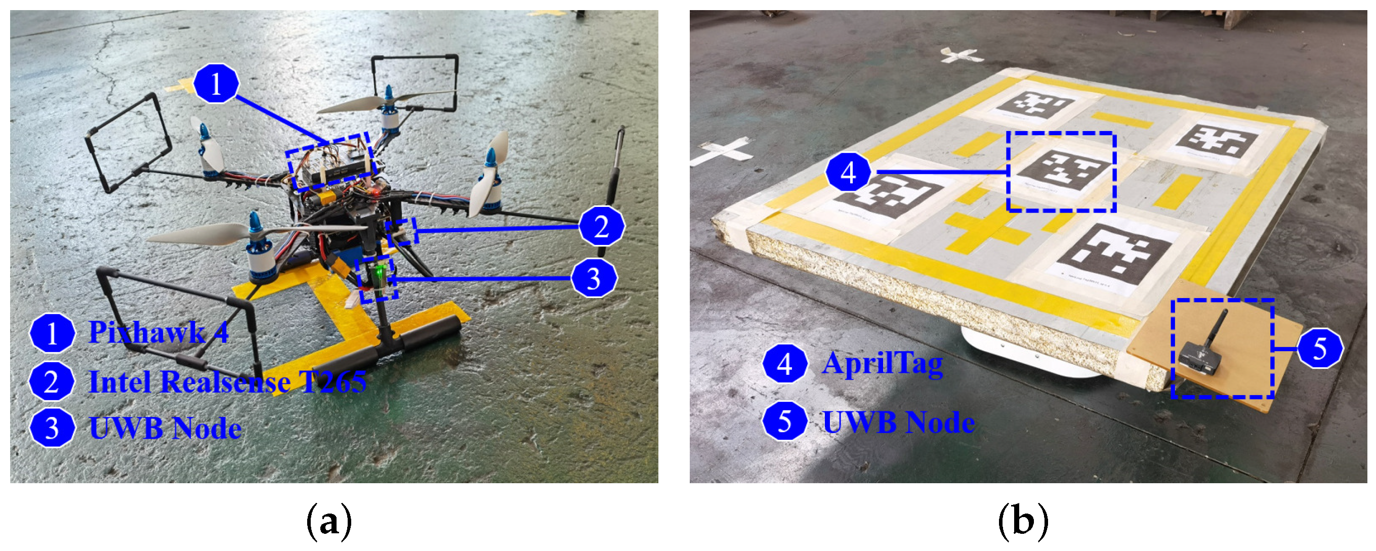
The UAV is equipped with one UWB node, a flight control computer that incorporates an inertial IMU and a camera mounted directly beneath its fuselage. The UGV is equipped with one UWB node, an IMU and encoders, which provide its motion state information. Note that the UWB node enables distance measurements between the UAV and UGV through bidirectional time of flight (TWTOF). Additionally, UWB can also be utilized for data communication between the UAV and UGV.
For autonomous docking in GPS-denied environments, there have been numerous works on precise landing, but docking with minimal deployment costs remains a challenge. The focus of this article is on navigation, so the impact of uneven ground is ignored.
2.1. UAV and UGV Models
Consider a situation wherein the UAV is docking with a UGV on a plane. To simplify the computational requirements for solving the problem, we consider that a low-level trajectory tracking controller is sufficient, eliminating the need to include roll and pitch in the dynamics. Thus, the model of the UAV can be described as follows [
31]:
where
and
represent the position and yaw angle of the UAV in the
frame, respectively;
is the
all-zero matrix;
is the rotation matrix from
to
; and
and
are the
frame linear velocity and angular rates, which are the control inputs.
Similarly, the model of the two-wheeled UGV is given as follows [
32,
33]:
where
t is time and
is the yaw angle of UGV with respect to
. The UGV moves in a plane, so its height is a constant (e.g., zero).
and
are the linear and angular velocities, respectively;
and
are the mass and moment of inertia of the UGV, respectively;
l and
r are the distance between the two wheels and the radius of the wheel, respectively; and
and
are the torques of the right and left wheels, respectively. In addition, it is worth noting that the linear velocity,
, and angular velocity,
, of the UGV can be expressed as follows:
where
and
are the velocities of the left and right wheels of the UGV, respectively.
and
are mutually independent random variables representing additive process noise to the left and right wheels, respectively. After the 2D UGV model is extended to 3D, the following dynamic model can be obtained:
where
is the position of the UGV at time instant
with respect to
,
, and
is the rotation matrix of
relative to
.
Remark 1. It should be noted that the situation considered in this paper is, ideally, flat ground without obstacles. Therefore, the UAV can use vertical take-off and landing methods without considering the roll and pitch angles, and the UGV does not need to consider the roll, pitch, and altitude changes that may occur. Of course, for some real-world scenarios, a road may not be flat. In this situation, especially landing, it needs to consider roll and pitch.
2.2. Relative Attitude Relationship of Two Vehicles
In order to achieve target docking, the relative attitude relationship between the UAV and UGV needs to be analyzed as follows. In the following, the continuous time is sampled by a sampling period,
, and the instant,
, is abbreviated by
k for all
. As shown in
Figure 2, the local pose of the target with respect to the UAV can be given as follows:
where
and
are the relative position and yaw angle between the UAV and UGV, respectively. By combining the above two equations with the discretization of Equations (
1) and (
4), after some manipulation, one can obtain the following:
where
and
are the position and yaw angle process noise at time instant
, respectively, such as wind turbulence affecting the UAV and UGV.
Note that when the UGV does not enter the FOV of the camera, the true distance can be expressed as follows: , where and are the measurement distance and noise, respectively.
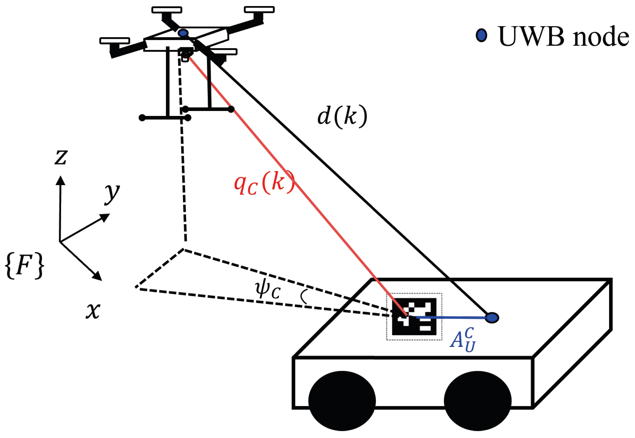
When the UAV enters the landing phase, as shown in
Figure 3, the vision sensor begins to recognize the AprilTag [
17] deployed on the UGV and detects the target point pose as follows:
where
and
are the relative yaw angle and position of the UGV obtained from the camera measurement and
is the measurement noise of the camera. For the measurement of
, vision-based methods are used for localization [
17], and the conversion relationship between the world coordinate
and camera coordinate
systems is given as follows:
where
and
are the rotation and offset matrices, respectively, which are obtained by camera calibration and internal parameters. In addition,
in
Figure 3 is the distance between the COMs of the UWB and AprilTag.
2.3. Control Objectives
The three control objectives used in this study are introduced below.
Problem 1.
(The localization phase). The objective of this phase is to compute the transition matrix, , and the relative position, , while controlling the UAV to take off at a uniform speed.
Problem 2.
(The navigation phase). The goal of this control phase is to design a controller for driving the UAV close to the UGV and making the UGV enter the FOV of the UAV, so as to meet the following conditions:where is a constant, representing the maximal FOV of the UAV. Problem 3.
(The landing phase). In this phase, the UGV is already in the FOV of the UAV’s camera. The Vision-IMU-UWB fusion navigation mode is enabled to design a controller with the target of landing control, i.e., Remark 2. During the first two phases, the UAV obtains its own displacement through visual–inertial odometry (VIO) using a vision sensor and IMU, and UWB can provide the speed and yaw angle of UGV while obtaining the relative distance. When switching to landing mode, vision will be switched from VIO to AprilTag for landing by fusing Vision-IMU-UWB information.
3. Navigation Control Design
Under the following assumptions, this section will study the navigation docking and autonomous landing control of a UAV on a mobile UGV.
Assumption 1. For the UAV and UGV in a 3D space, the linear and angular velocities of both vehicles are bounded, that is, , , and . In addition, in order for the UAV to dock with the UGV, and are also assumed.
Assumption 2. In the first two phases, the UAV and UGV are within range of the UWB sensors. In the process of autonomous landing, the UAV can always detect the AprilTag on the UGV.
This study examines autonomous docking under non-cooperative conditions. Therefore, in an actual engineering context, the motion performance of the UAV is better than that of the UGV, and the speed variation in the UGV is usually small when entering the landing phase, so Assumptions 1–2 are reasonable.
Figure 4 shows the framework of the entire autonomous docking. In this framework, UAVs and UGVs perform measurements through their own sensors, and all measured data are processed by the UAV’s on-board computer. The autonomous docking framework includes the take-off, navigation and landing phases, and the specific implementation process will be presented in
Section 3.1,
Section 3.2 and
Section 3.3.
3.1. Take-Off Positioning Phase
According to the framework designed in the previous section, the required relative position,
, and conversion matrix,
, of
relative to
are obtained through the measured data of UAV in the take-off phase. As shown in
Figure 5, when the UAV takes off vertically at a constant speed, its VIO obtains altitude, UGV displacement (determined by the UGV speed and yaw angle) and their distance information
through UWB. By projecting the spatial relationships onto the
-plane, we establish the Cayley–Menger determinant [
34] relationship at time instants 0 and 1 as follows:
Hence, we can determine the angles, and , that describe the geometric relationship between the two. Moreover, considering the deviation in the angles between them at this instant, we installed a UWB sensor in the forward direction of the UAV and another UWB sensor at the front of the UGV. Utilizing the relationship between their signal strengths, we can derive the actual relative position between the UAV and UGV.
Remark 3. In projection, the height sensor is used to calculate , where is the z axis coordinate of the UAV. In summary, the relative position relationship and transformation matrix in the coordinate system are mainly solved using the above geometric methods. After obtaining the relative position, based on previous work [35], the angle between the forward directions of the two UWB sensors can be calculated using UWB signal strength, thereby determining the transformation matrix, , and the relative position coordinates in . 3.2. Navigation Control Algorithm
In this section, we will directly refer to
Figure 6 to describe the main idea of completing the navigation task. With the preparation for navigation in the take-off stage and considering the position information, an inverse proportional saturation controller is designed as follows:
where
denotes the estimate of
to be introduced later;
;
is the rotation matrix from
to
; the yaw angle,
, is not considered at this stage for the time being; and
represents the larger value between
A and
B. Note that the controller, at this time, mainly controls the quantities in the
-plane, and the height control is zero. Finally, the obtained control signal,
, is transmitted to the UAV through the flight control computer, enabling the control of the UAV in the body coordinate system.
As shown in
Figure 2, by using the displacement relationship between UAVs and unmanned ground vehicles in space, the following results can be obtained:
where
is the measurement noise of UWB, which is a random noise sequence that satisfies the following assumptions.
Assumption 3. There exists a constant, , such that the measurement noise, , satisfies the following: Remark 4. is the error generated by the UWB sensor through measurements that are within 10 cm and independently uncorrelated for each moment.
The following equation can be obtained using Equations (
13) and (
14):
With the above relationship, let us define
Using Equation (
17), one then has the following:
which will later be employed to estimate
.
Remark 5. For in Equation (17), through , the following can be obtained:where, by defining , the term has a mean of 0 and takes values from the interval . In addition, is a random noise with a mean of zero and takes values from the interval . Therefore, is regarded as a noise random sequence with zero mean value and takes values from the interval . To proceed, let us first define the following parameters:
where
p is the horizon of multiple innovation,
and
N is an integer.
Therefore, the cost function can be constructed through Equations (
20)–(
22), as follows:
where the above formula is the expectation of a square error. Then, by minimizing the cost function, the approximation algorithm is proposed as follows:
where
is an innovation vector, namely, multi-innovation. Equations (
20)–(
22), (
24) and (
25) are called the MIFG algorithm.
Lemma 1. For Equation (22), if the information vector, , in Equation (17) is persistently excited, that is, there exists and and an integer, , such that the following holds:and , and if , then satisfies the following: Remark 6. Compared with the simple use of two groups of data, such as estimating the relative position, , increasing the innovation horizon, p, will lead to a smaller relative position estimation error. However, a larger p will inevitably incur a heavier computational power, which should be a tradeoff in practical implementations.
Assumption 4. The relative position changing rate, , of the UAV and UGV, is uncorrelated with for . At the same time, the changing rate should be square-bounded, i.e., and , for some . In addition, it is assumed that and are independent, i.e., .
With the above preparation, it is now possible to present the first main result of this study, which is the convergence of the proposed multi-innovation forgetting gradient (MIFG) algorithm.
Theorem 1. For Equations (24) and (25), let Assumptions 1, 3 and 4 hold, and the innovation horizon . Then, the estimation error given by the MIFG algorithm satisfies the following: Remark 7. The physical meaning of Theorem 1 is that the error between the estimated relative position, , obtained by MIFG and the true relative position, , is bounded.
Remark 8. Compared with the literature relying on GPS information [9,36,37] or MCS [38,39,40] for positioning, the method in this study uses only a range sensor and its odometer to achieve navigation and positioning at a minimum deployment cost. Compared with relative positioning based on visual search, the method here has wider-range measurements, shorter searching times and requires fewer computing resources. Compared with [29,30], this study considers a dynamic random target. Compared with [28], we consider the measurement error and use historical data for estimation in control. 3.3. Multi-Sensor Fusion Landing Scheme
This subsection focuses on the case where the UGV appears in the FOV of the camera. The pose of the target is obtained by fusing multiple sensors, and the landing is completed by designing a controller.
As shown in
Figure 7, the overall idea is to fuse the Vision-UWB-IMU data based on the EKF to obtain the relative position coordinates between the UAV and UGV for landing control.
Assumption 5. In the landing phase, it is assumed that a change in vehicle speed can be ignored. In addition, the distance measured by UWB is the same as the distance measured by vision, that is, the position of the tag and UWB node are regarded as the same position on the UGV.
To proceed, define the following:
where
represents the relative position of the UAV to the landing site and
indicates the relative heading angle of the UAV to the landing point. Moreover, the dynamics of
in
can be compactly written as follows:
, where
f denotes the evolution function of
and
represents the system noise.
For a precise landing, the landing point is selected differently from the UWB location. According to
Figure 3, the relative position estimated by the UWB sensor at this moment is as follows:
The next step is to use the EKF method to fuse the on-board IMU/encoder, vision sensor and UWB data to obtain the following:
where
,
and
are position components of the estimated relative position and
represents the estimated relative yaw angle. In particular, the camera sensor will obtain the relative position and yaw angle between the UAV and AprilTag; the UWB continues to be used to estimate relative positions, as performed previously; and the IMU/encoder can obtain the relative velocity, position and angle between the UAV and UGV.
Remark 9. The EKF method has been widely used for different sensors in engineering applications and has been verified to be a better method in practice, so this study does not introduce the algorithm in detail [41,42]. Note that data are obtained from both the UAV’s IMU and UGV’s IMU/encoder, which are not presented in this study and can be found in [41]. After obtaining the relative position,
, of multi-sensor fusion, the controller is designed to track the position in
x and
y directions and compensate the UGV’s velocity as follows:
where
is the transformation matrix from
into
. Note that, unlike the navigation phase, the UAV controller is designed based on position control and
where
is a prespecified falling average height. Then, finally, when the estimated relative height,
, reaches a certain threshold value, i.e., satisfies the landing altitude, the UAV power is cut off to complete the landing.
Remark 10. The main contribution of this subsection is that compared with the method of relative positioning using only vision [13,17,43], the data fusion estimation of relative positioning combined with UWB, IMU, and the encoder is carried out, and the higher positioning accuracy is demonstrated using a numerical simulation. Moreover, an unmanned landing controller based on spatial location information is designed. 


