Article

An Autonomous Tracking and Landing Method for Unmanned Aerial Vehicles Based on Visual Navigation

1
Key Laboratory of CNC Equipment Reliability, Ministry of Education, School of Mechanical and Aero-Space Engineering, Jilin University, Changchun 130022, China
2
Chongqing Research Institute, Jilin University, Chongqing 401123, China
*
Authors to whom correspondence should be addressed.
Drones 2023, 7(12), 703; https://doi.org/10.3390/drones7120703
Submission received: 26 October 2023 / Revised: 8 December 2023 / Accepted: 11 December 2023 / Published: 12 December 2023

Abstract

:
In this paper, we examine potential methods for autonomously tracking and landing multi-rotor unmanned aerial vehicles (UAVs), a complex yet essential problem. Autonomous tracking and landing control technology utilizes visual navigation, relying solely on vision and landmarks to track targets and achieve autonomous landing. This technology improves the UAV’s environment perception and autonomous flight capabilities in GPS-free scenarios. In particular, we are researching tracking and landing as a cohesive unit, devising a switching plan for various UAV tracking and landing modes, and creating a flight controller that has an inner and outer loop structure based on relative position estimation. The inner and outer nested markers aid in the autonomous tracking and landing of UAVs. Optimal parameters are determined via optimized experiments on the measurements of the inner and outer markers. An indoor experimental platform for tracking and landing UAVs was established. Tracking performance was verified by tracking three trajectories of an unmanned ground vehicle (UGV) at varying speeds, and landing accuracy was confirmed through static and dynamic landing experiments. The experimental results show that the proposed scheme has good dynamic tracking and landing performance.

1. Introduction

UAVs offer numerous advantages, such as strong maneuverability, low maintenance costs, vertical takeoff ability, and impressive hovering capabilities. As a result, they are widely used in various fields, including search and rescue, exploration, disaster monitoring, inspection, and agriculture [1,2,3,4]. However, limitations on payload and flight time significantly restrict the range of UAV missions. Therefore, it is essential to develop fully autonomous multi-rotor UAVs that can collaborate with ground-based robots to perform more complex tasks [5,6]. In this case, especially during the takeoff and landing phases, high-precision vehicle position and attitude estimation and motion planning are required [7,8].
In recent years, scholars globally have extensively researched UAV tracking [9,10] and landing techniques [11], for instance, identifying safe landing locations using visual cues following a severe UAV malfunction [12]. Landing a UAV on an unmanned vessel is a challenging problem [13,14,15]. The fluctuating water surface causes unpredictable changes in the position and attitude of the unmanned vessel. Landing the UAV on the UGV can give the UGV system the ability to work in a three-dimensional space, and carrying the charging module on the UGV can solve the limitations of payload and flight time on the working range of the UAV, but it places high requirements on the accuracy of the drone landing [16,17,18,19]. The position and attitude of a UAV are estimated during the landing process, but the position and attitude of today’s UAVs are typically measured by inertial measurement units (IMUs) and Global Positioning System (GPS) [20]. However, the positioning accuracy of GPS is low, and it is not possible to use GPS positioning indoors or in places with a lot of cover. IMUs have the problem of accumulating errors in long-term positioning, making it difficult to perform high-precision tasks such as landing. Therefore, the selection of sensors is particularly important when the UAV performs the landing mission. Laser sensors can provide accurate distance information, accurately calculate the relative position and attitude relationship between the UAV and the landing landmark, and are used in UAV landing missions [14]. However, laser sensors are expensive, require a large amount of data, and have high platform requirements, making them unsuitable for mounting on small multi-rotor UAVs.
With the advantages of easy maintenance, low price, miniaturization, light weight, and low power consumption, vision sensors are widely used in various intelligent robots. With the development of technology, UAV visual localization can provide precise position and angle information, which can meet the accuracy requirements of UAV landing guidance. However, accurate landmark recognition is a challenge, and edge detection algorithms [21,22] and deep learning methods [19] are commonly used. These methods are computationally intensive and poorly portable, and deep learning also requires large amounts of data. Optical flow is also a promising solution for autonomous landing missions [23], but it is less stable as it is highly dependent on the environment.
During UAV landings, as the visual sensor approaches the landing landmark, there is a risk of losing information on global and relative position and attitude information, resulting in decreased landing precision or even failure. Therefore, a precise landmark must be designed to guide the UAV towards a successful landing. The use of ArUco marker is a common method for guiding UAV landings [17,18,19]. Compared to other markers, such as AprilTags and ARTags, ArUco markers can be easily generated and recognized using OpenCV. Ref. [24] compares AprilTags, ARTags, and ArUco markers in terms of recognition distance, accuracy, and computing resource consumption. ArUco markers have a low probability of detection errors during the recognition process and are therefore straightforward to set up and robust in tracking and landing UAVs. Therefore, we use the ArUco marker as landmark. When utilizing an ArUco marker for UAV landing guidance, the global information of the marker is forfeited when the UAV landmarks are in close proximity. As a result, nested ArUco markers or ArUco marker matrices are commonly implemented to ensure the precision of the low-altitude relative positions and attitudes of the UAV during landing.
This paper’s primary contribution is the development of dynamic tracking and landing control strategies for UAVs and the optimization of landmark structure and dimensions to obtain the best possible landmark parameters. By relying solely on vision to achieve dynamic tracking and precise landing of UAVs, an experimental platform for indoor UAV tracking and landing was established. The UAV tracking performance was validated by tracing three different trajectories of the unmanned ground vehicle (UGV) at varying speeds, while the landing precision of the UAV was confirmed through both static and dynamic landing experiments.

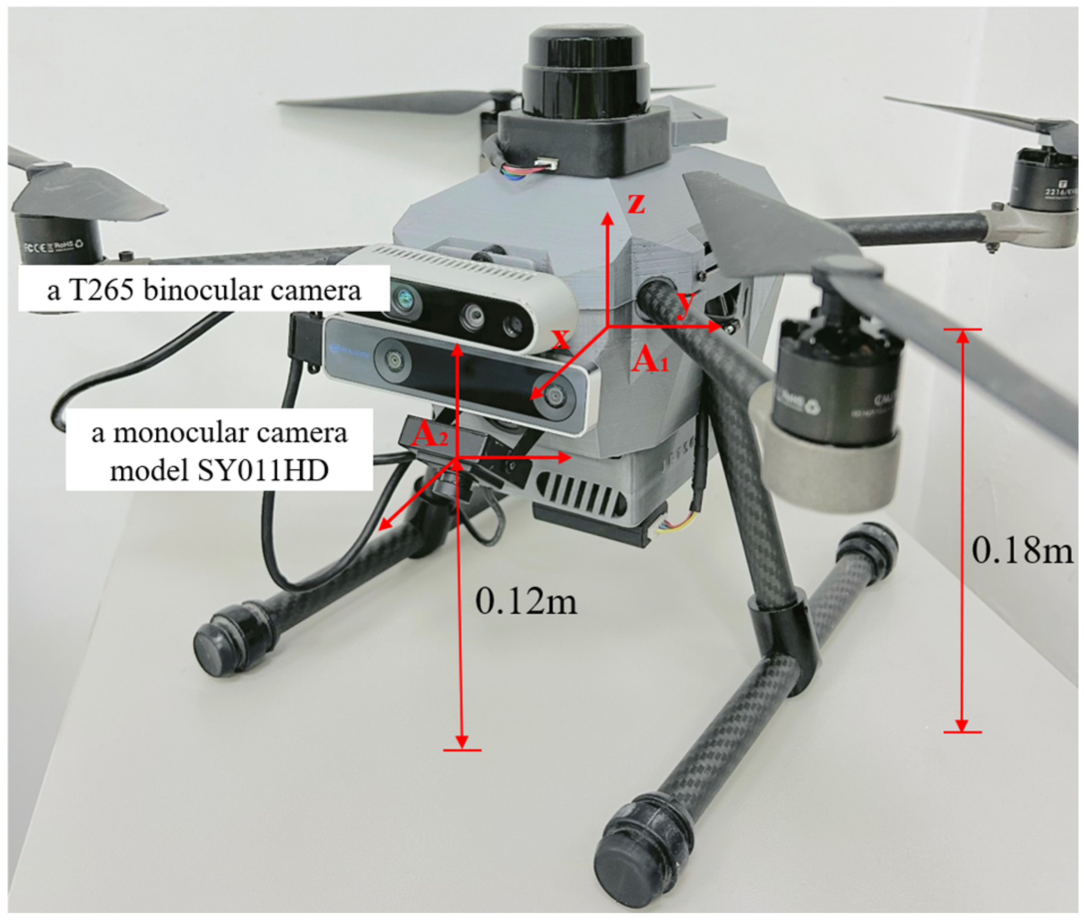
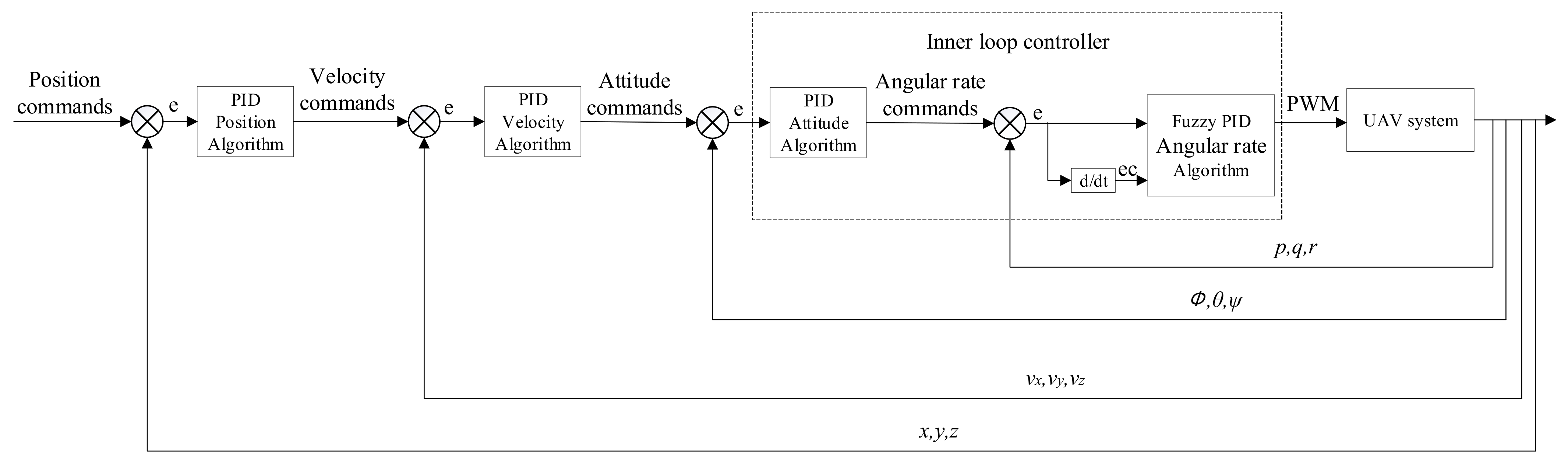
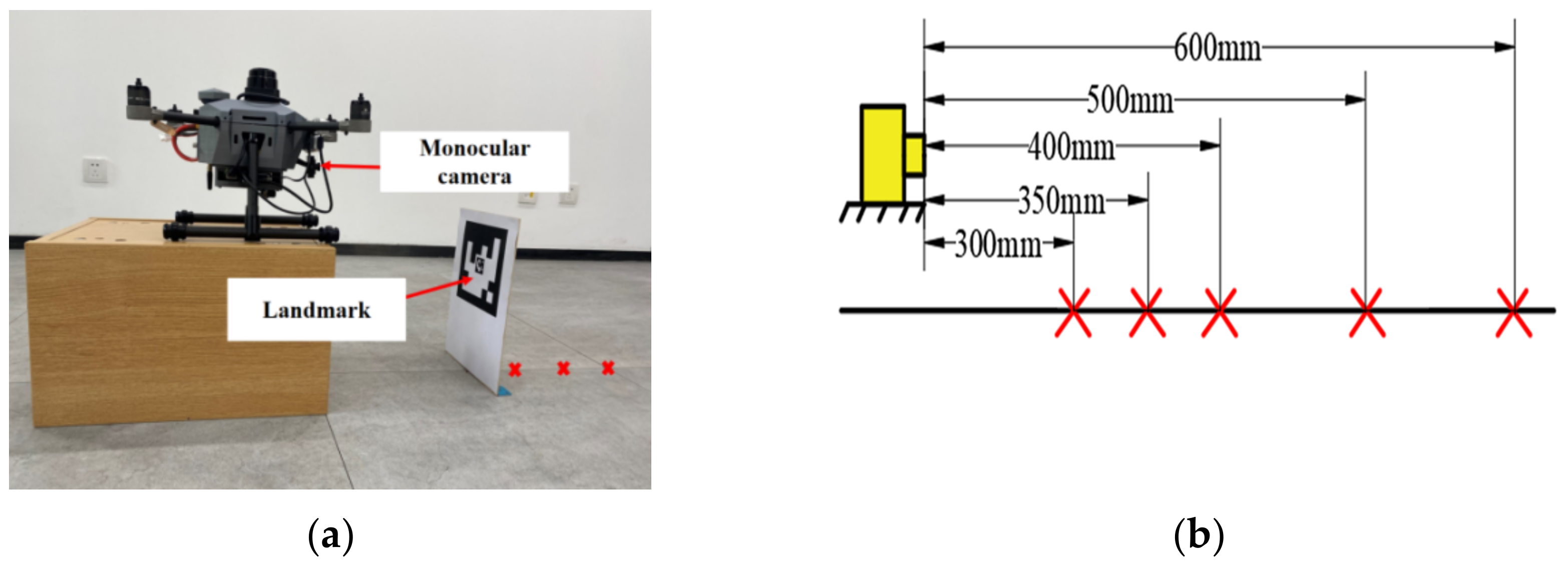
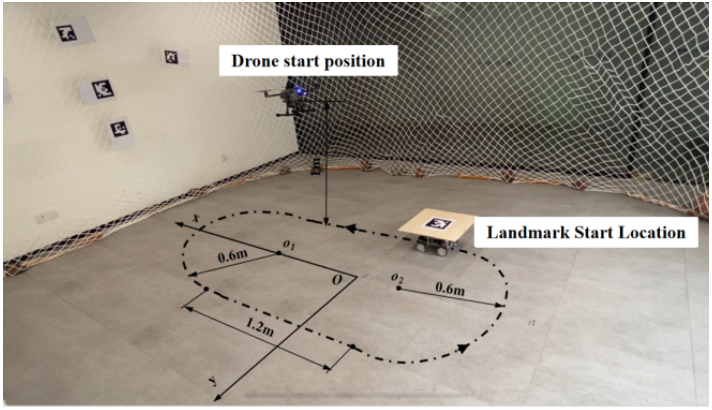
2. Materials and Methods

During the dynamic tracking and landing of the UAV, the state of the UAV is categorized into a tracking mode and a landing mode based on the relative position and attitude of the UAV and the landmark carried by the UGV (shown in Figure 1). Initially, the UAV utilizes vision to gather details about the surrounding area. If a landmark is identified, the UAV calculates the relative positions and attitudes of itself and the landmark. If no landmark is detected, the UAV will automatically elevate its altitude to broaden its field of view and locate the landmark. The controller receives the relative position and attitude obtained and translates it into commands to control the UAV. In tracking mode, the UAV sends commands to control the horizontal channel to the UAV’s flight controller to guide the UAV horizontally close to landmarks for autonomous UAV tracking, maintaining the UAV’s altitude to keep the target in view and adjusting the UAV’s speed to keep up with the target. The UAV enters the landing mode when the relative positions and attitudes of the UAV and the landmark meet the landing conditions. In landing mode, the UAV approaches the landmark horizontally, dropping its own altitude and keeping the UGV at the same speed as the tracked target; if the target is lost, it rises to expand the field of view to bring the target back into view; if the target is not lost, it calculates the straight-line distance to the center of the landmark. This straight-line distance refers to the distance from the center of the UAV to the center of the landmark(shown in Figure 2). When the straight-line distance is less than 0.3 m, the UAV’s landing command is triggered: the motor decelerates to land the UAV.
To fulfill the demands of the tracking and landing mission, the UAV is controlled through a controller featuring an inner and outer loop structure (shown in Figure 3). The inner loop structure controls the attitude angles ϕ, θ, ψ, and angular velocities p, q, r. An algorithm incorporating fuzzy PID is utilized for the attitude angular velocities, and a cascaded PID control regulates the attitude angles. Step response experiments were conducted in the MATLAB simulation platform for pitch angle, roll angle, yaw angle, and the corresponding angular velocity. The desired values were set to 0.1 for both the angle and angular velocity, with a simulation step size of 1 ms. The step response performance metrics were calculated from the step response curves: rise time “tr”, regulation time “ts”, peak time “tp”, and maximum overshoot “σ” (Table 1). The cascaded PID control algorithm is used in the outer loop structure to control the UAV’s position. The position controller comprises two loops to control speed and position. Simulation experiments were conducted on the system to track a circular trajectory with a 3 m radius. The desired positions of the x and y axes are updated at a rate of 0.2 radians per second (shown in Figure 4). The three-axis position response curves can be obtained. The resulting position response corresponds closely to the expected value, with a slight degree of hysteresis that produces an error of approximately 0.6 m. The z-axis position response is comparatively faster than the x and y axes’ responses. Consequently, the tracking effect of the system essentially meets the requirements.
Using only visual information for autonomous UAV tracking and landing in GPS-less environments requires both estimating the position and attitude of the UAV itself based on visual navigation techniques, and detecting and tracking landmarks to achieve a landing. Therefore, the UAV has to carry two cameras, the first with a T265 binocular camera from Intel for localization and the second with a monocular camera model SY011HD for target tracking. Figure 2 shows the mounting position of the two cameras on the UAV, and some performance parameters of the two cameras are shown in Table 2.
In this experimental research, we use the landmark generated by the ArUco library provided by OpenCV to guide the UAV to perform a tracking landing task. The inner and outer nested landmarks were used (shown in Figure 5), the landmarks were parameterized, and landmark parameter optimization experiments were performed to derive the optimal landmark parameters.
A black box surrounds each landmark, which initially detects quad candidates. Through inner and outer nested landmarks, up to two quads can be detected. When the camera detects two markers simultaneously, it independently calculates the contour perimeter of each marker and selects the quadrilateral marker with the smaller perimeter. In other words, the target is tracked and landed using information from the inner landmark. This approach increases the likelihood of maintaining the landmark within the camera’s field of view. When the camera is too close to the landmark, the outer marker occupies a larger area in the field of view and is more likely to lose global information, leading to a higher chance of losing the target and hindering the UAV’s landing. For the selected quadrilateral marker, we conduct a decoding operation. If the decoding is successful, it confirms the landmark as the target. Subsequently, we obtain the relevant information including the landmark, corresponding contour, and corner points. This information aids in determining the relative position of the UAV in relation to the landmark.
In the UAV tracking landing missions, landmark failure typically occurs at the time of touchdown. While the relative distance between the UAV and the landmark in the height direction in the landing mode is between 0.3 and 0.6 m, the variation of the relative distance between the UAV and the landmark in the landmark parameter optimization experiments is therefore set in the range of 0.3 to 0.6 m (shown in Figure 6). The UAV uses vision to measure the relative distance between the UAV and inner and outer markers of varying sizes. The position of the UAV does not move, changing the position of the landmark. The red “x” in the graph indicates each position of the landmark in the experiment, and the results of three experiments were recorded at each position. Table 3 shows the estimated relative distances for inner markers of different sizes. Table 4 shows the estimated relative distances for outer markers of different sizes. During the experiment aimed at calculating the dimensional parameters of the outer marker, no inner marker was present.
To achieve more accurate landings, it is necessary for the relative position estimation data to possess a higher level of accuracy as the distance between the UAV and the landmark decreases. Based on data in the table, the relative distance derived from the inner marker of size 30 mm × 30 mm is closer to the actual value when the relative distance is small. Although the UAV cannot detect the inner marker measuring 30 mm × 30 mm at long distances, it can still obtain relative position information by recognizing the outer marker, which follows the sequence of landmark recognition in real-world scenarios. An outer marker with a size of 150 × 150 mm was chosen for more precise relative position estimation at smaller distances. The optimal nested landmark parameters are then determined (shown in Figure 7).
We designed the hardware platform for the tracking and landing system (shown in Figure 8). We used the Robot Operating System (ROS) as the backbone of the software and control. The UAV features a high-speed monocular camera model SY011HD and a binocular T265 camera, an on-board processor, the Nvidia-developed Jetson Xavier NX board, and flight controllers utilizing the Pixhawk4 hardware. In this system, the ground PC logs in remotely via WiFi to the onboard processor Jetson Xavier NX. The UAV’s onboard processor retrieves the UAV’s status information from the T265 camera via the ROS system. Concurrently, the SY011HD monocular camera transmits captured image information to the processor. Landmark identification occurs, and the relative positions between the UAV and the ground landmark are calculated to extract pertinent control information. The UAV is able to execute tracking and landing tasks by receiving control commands transmitted via the MAVROS package to its flight controller.

3. Results

Indoor flight experiments on UAV tracking landings were conducted in this research. The experimental scenario can be seen in Figure 9, which includes a quadcopter UAV with a wheelbase of 450 mm, a ground-based UGV, and a landing platform with the nested ArUco markers. A protective net was constructed around the experimental site’s perimeter, and ArUco markers were affixed to the net to enhance the UAV’s positional accuracy. A coordinate system was established at the experimental site, as depicted in Figure 9. We conduct experiments to track the flight of ArUco markers that move with the UGV’s three types of motion: linear reciprocating, circular, and straight-sided elliptical. In the experimental scenario, we plotted the motion trajectories of the UGV on the ground for three different paths to verify its position reliability. During the experiments, the UGV’s position and speed data are sourced from the wheel speed odometer, while UAV’s position and attitude information is obtained from the T265 camera. Inevitably, the UAV and UGV inherently generate a positioning measurement error. The auxiliary positioning ArUco markers present on the protective net serve the purpose of providing as much visual feature information as possible to the T265 binocular camera. Before the experiment, we conducted calibration experiments on the wheel speed odometer with the three motion trajectories of the UGV, respectively, compared the true value of the ground trajectory with the data measured by the odometer, and calibrated the cumulative error of the wheel speed odometer, so as to obtain more truthful information about the position of the UGV. Since the wheel speed odometer is calibrated to measure the UGV position very accurately, there is no requirement for an external measurement system to position the UGV. It will not affect the comparison with the experimental results. The offset of the initial UAV and UGV positions from the origin of the defined coordinate system were recorded prior to the experiment’s commencement. Since the position and attitude transformations of UAV and UGV are based on the body coordinate system, and the position information is recorded with its own starting point as the origin, the position information of the two in the same coordinate system can be obtained by making a difference between the data recorded by the two and the deviation of their respective initial positions.
During the experiment, in order to verify the effectiveness of UAV tracking and landing, we investigated the relative position deviation and velocity deviation between the UAV and UGV. Part of the bias arises from the algorithmic bias produced during the tracking process, and the other part of the bias derives from the dynamic response bias of the control system. Prior to the experiment, we optimized the parameters of the flight controller. Since we are focused on implementing a comprehensive method for vision-based tracking and landing of UAVs, we only analyze the overall bias generated by the tracking and landing system. The UGV was made to move at three speeds, v1 = 0.2 m/s, v2 = 0.4 m/s, and v3 = 0.6 m/s, while performing three different forms of motion in order to test the robustness and accuracy of the UAV’s dynamic tracking and landing.

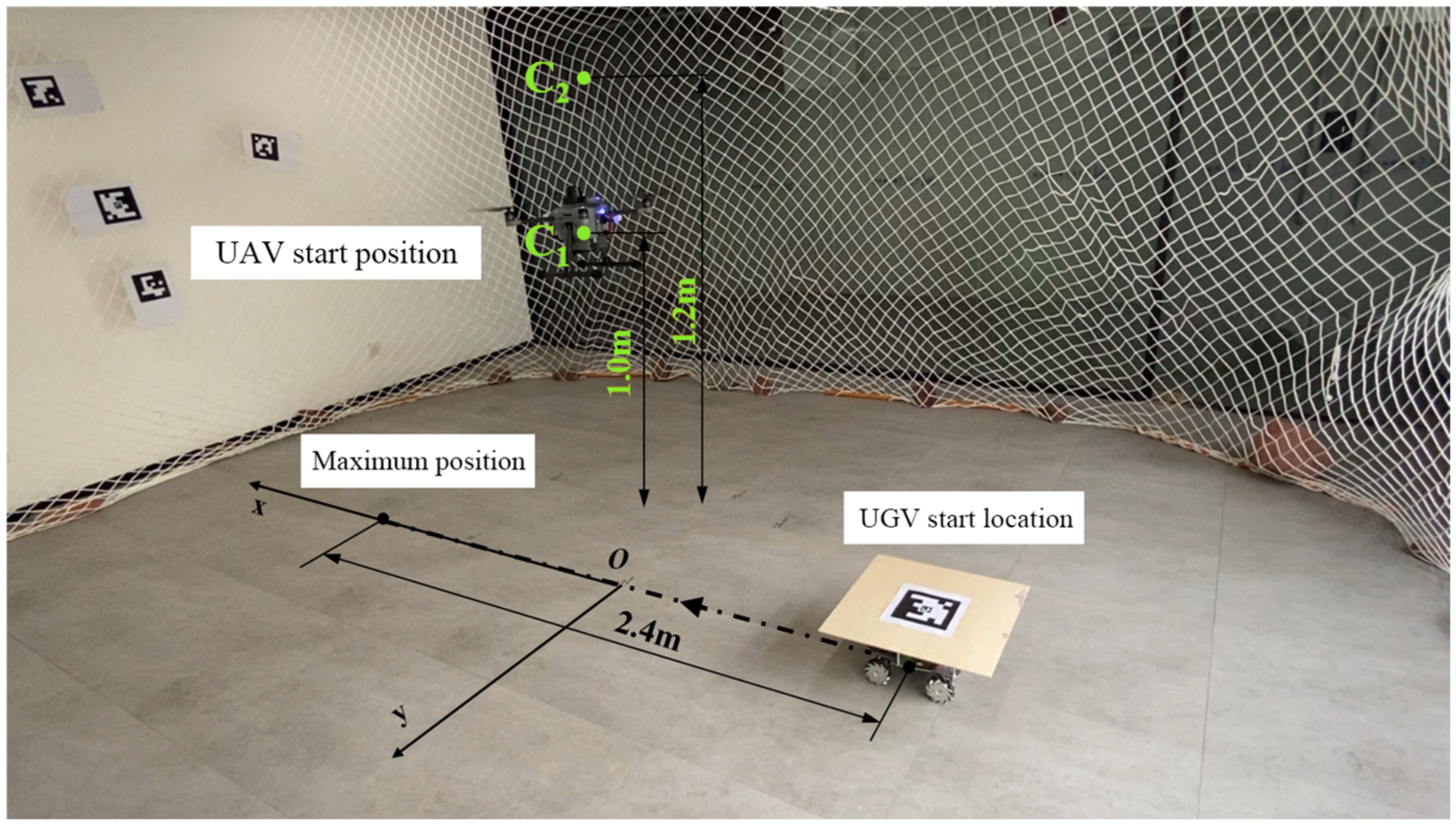
3.1. Tracking Experiments

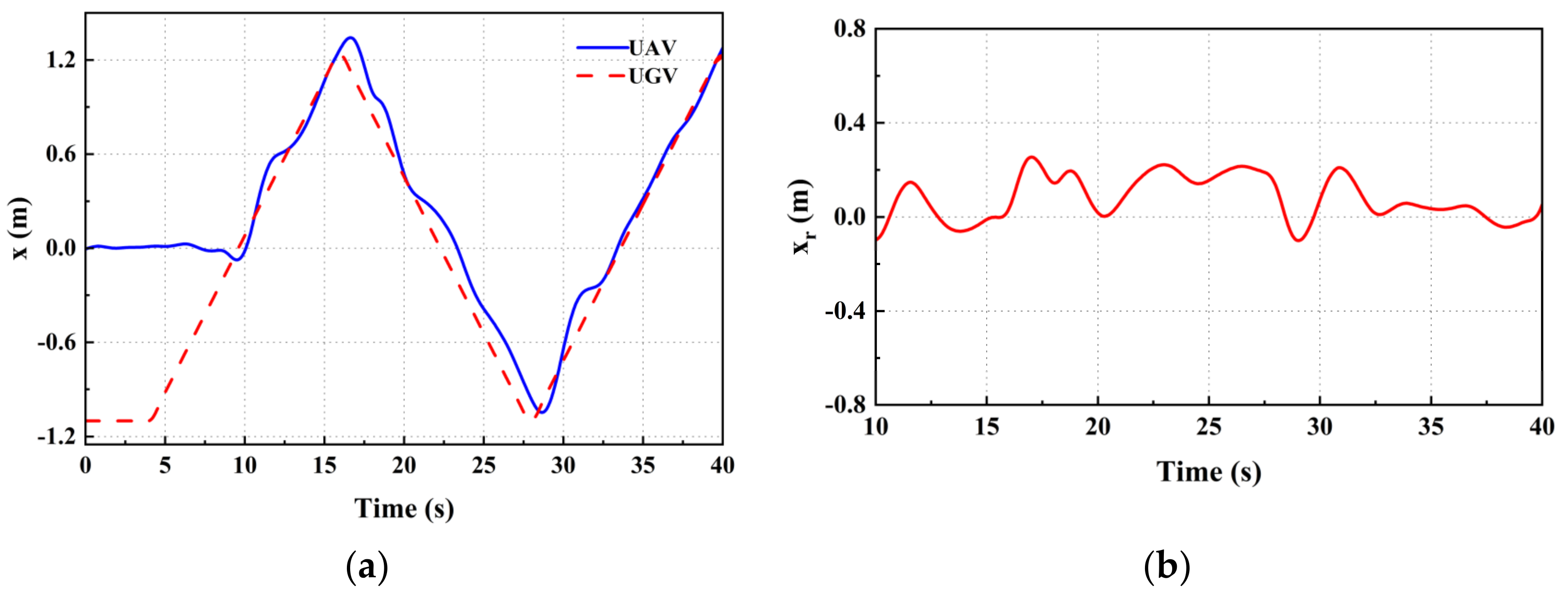
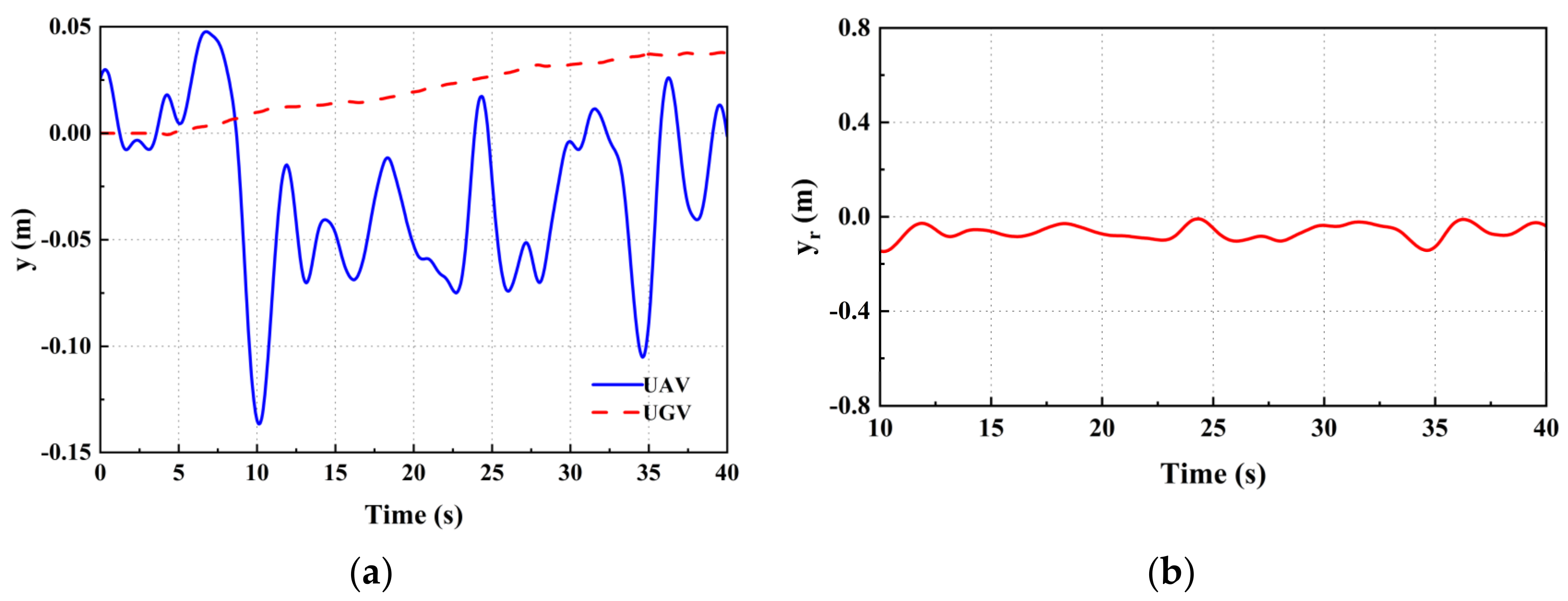
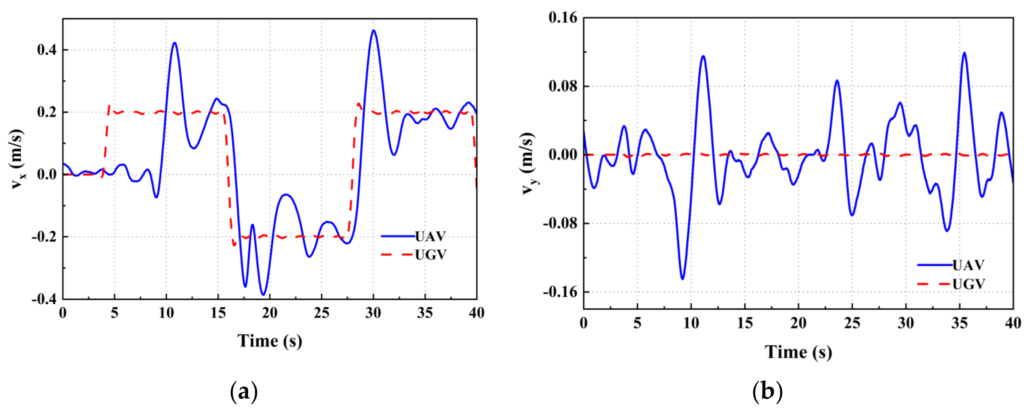
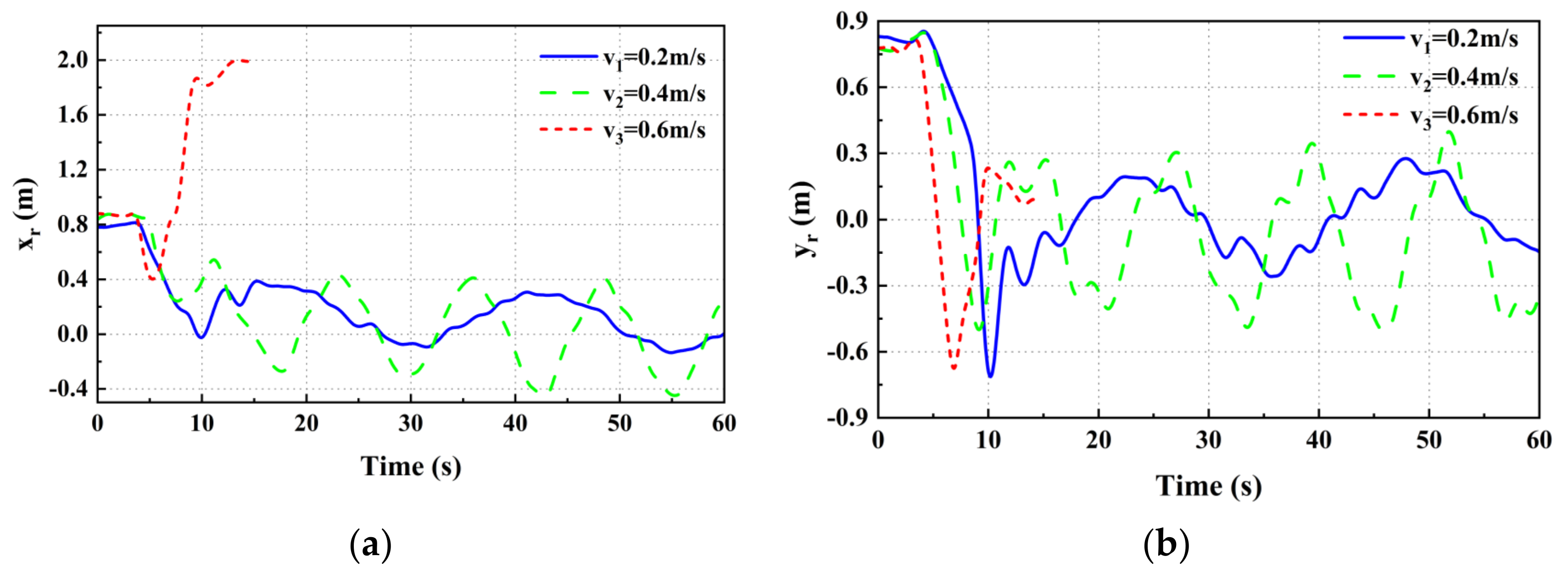
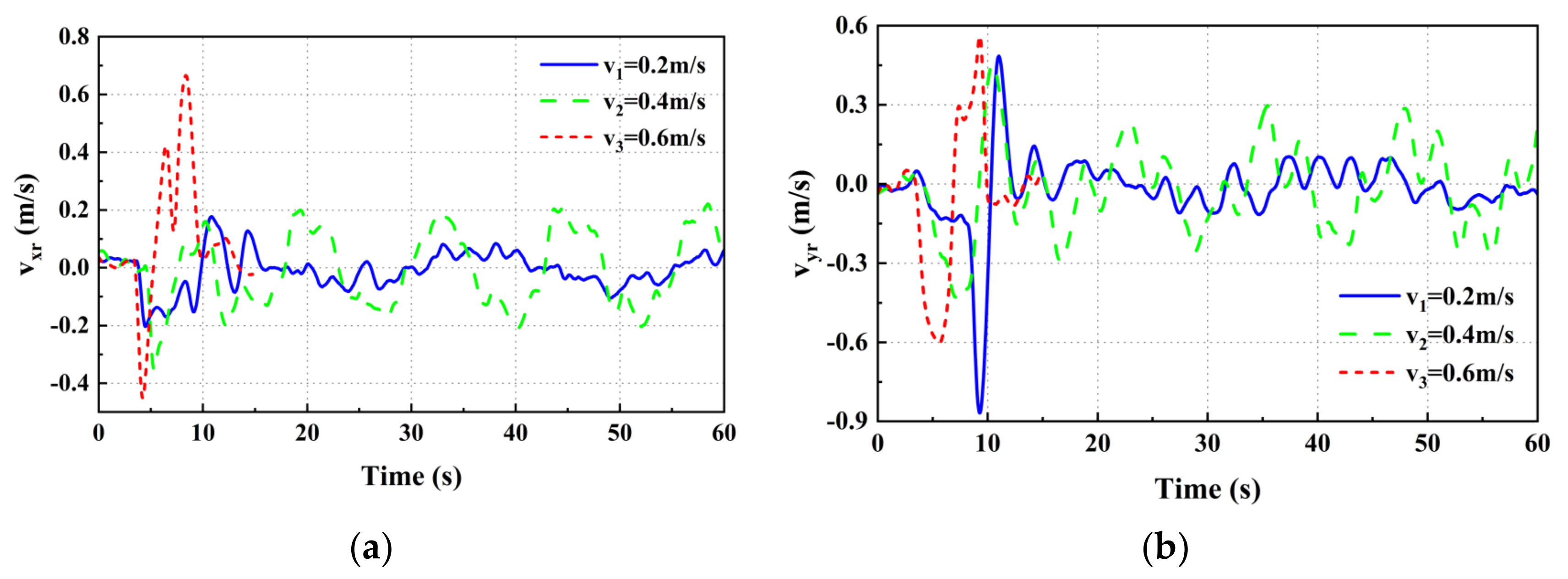
3.1.1. Linear Reciprocating Trajectory

In the experiment, landmarks follow the UGV while it moves in a straight reciprocating motion at three different speeds. This is done to verify the tracking performance of the UAV. Taking into account the influence of the UAV’s movement speed and camera field of view on tracking performance, we adjusted the starting point of the UAV’s tracking at different heights depending on the speed (shown in Figure 10).
When the UGV is moving at velocity v1, the UAV’s position relative to the UGV in the x and y axes can be obtained (Figure 11 and Figure 12). xr and yr represent the deviations of the UAV and UGV along the x and y axes, respectively. The speeds of the UAV and the UGV on the x and y axes are depicted in Figure 13. There was a momentary increase in the speed of the UAV at 10 s, attributed to the landmark entering the UAV’s field of view. The UAV’s speed overshooting at 18 s and 28 s recurs as a result of the UGV changing direction. To ensure timely tracking of the landmark, an appropriate value of proportional gain (Kp) is set in the velocity controller, which ensures that the UAV can keep up with the UGV but also ensures that the control system is not divergent. Therefore, the UAV is highly responsive to landmark velocity changes and the controller exhibits overshooting behavior. During stable tracking, the UAV’s linear velocities along the x and y axes fluctuate at a rate commensurate with the speed of the UGV motion attachment.
From Figure 14, we are able to obtain the positional deviation of both the UAV and UGV on the x and y axes while the UGV is moving at three distinct speeds, namely xr and yr. The UGV’s tracking was stable at speed v1 but failed to maintain stability for extended durations at speeds v2 and v3. The UAV was more susceptible to losing the target due to the experimental site’s limitations. The UAV flew at a lower altitude, and the camera’s field of view was smaller. The mean and the mean square deviation of positional deviations in the x and y axes during constant tracking at speeds v1 and v2 were calculated and presented in Table 5. The mean outcomes in the table indicate that there is a slight increase in positional deviation between the UAV and the UGV in both the x- and y-axis directions as the speed of UGV movement increases. However, it still remains at the decimeter level. The table’s mean square error results indicate a gradual increase in x-axis position deviation fluctuation with the UGV’s increasing speed, whereas the UGV’s speed does not have a direct relation to y-axis position deviation fluctuation.
From Figure 15, one can derive the velocity deviation between the UAV and UGV on the x and y axes, denoted as vxr and vyr, respectively, when the UAV moves at three distinct velocities. The mean squared sum of the difference in velocity between the UAV and the UGV in the x- and y-axis directions is computed for UGV velocities v1 and v2. The findings are presented in Table 6. When comparing the speed deviation fluctuations near 0 m/s at different speeds, it becomes more evident that the fluctuation near 0 m/s increases as the mean square sum of the speed deviation increases. As the UGV’s speed increases, the mean square sum of the deviation in the x-axis velocity also increases, resulting in more noticeable fluctuation. Meanwhile, the y-axis deviation fluctuation remains consistent near the speed of 0 m/s. One part of the deviation comes from the algorithmic error generated during the tracking process, while the other part of the deviation comes from the dynamic response error of the control system. We analyzed the overall system error. When the velocity of UGV is v1, the mean square error in the x-axis velocity is 0.013 m/s, and the mean square error in the y-axis velocity is 0.00189 m/s. When the velocity of UGV is v2, the mean square error in the x-axis velocity is 0.133 m/s, and the mean square error in the y-axis velocity is 0.0132 m/s.

3.1.2. Circular Trajectory

The UAV circular trajectory tracking experiment was performed in parallel to the linear reciprocating motion tracking experiment. The UGV moves in a circular motion, with a radius of 0.8 m, at three distinct velocities. Only the starting point coordinates for the UAV and UGV were altered in comparison to the linear reciprocal motion tracking experiment (shown in Figure 16).
We can determine the amount of deviation in position between the UAV and the UGV when the UGV is moving at three distinct speeds (shown in Figure 17). Achieving stable tracking is possible at UGV speeds v1 and v2; however, at speed v3, the target is lost around the 15th second, making it impossible to maintain stable tracking for a long time. The probable reason for this is the low flight altitude of the UAV, which narrows the field of view of the camera and thereby increases the chances of target loss. The mean and mean square deviation of the position deviation of the UAV and the UGV were calculated and the results are shown in Table 7. It can be concluded that as the speed of the UGV increases, the mean position error and the mean square error of the x and y axes increase to a certain extent, i.e., the position error and the degree of fluctuation of the position error are positively correlated with the speed of the UGV. Furthermore, when compared with Table 5, the mean value of the x-axis position deviation for the UGV making a circular motion at the same speed is smaller. And since the UGV has a y-axis velocity in the circular motion, the mean and the mean square of the y-axis position deviation are larger in the circular motion.
We can obtain the velocity deviation between the UAV and the UGV on the x and y axes when the UGV is moving at three different speeds (shown in Figure 18). The mean square sum of the velocity deviations was calculated and the results are shown in Table 8. The fluctuation of UAV and UGV speed deviation becomes more noticeable as the speed of the UGV increases. Compared to Table 6, the fluctuation of the velocity deviation in the x-axis direction is smaller for the same velocity in circular motion. At the same time, since the UGV has a y-axis velocity during its circular motion, the phenomenon of fluctuating velocity deviation in the y-axis direction between the UAV and the UGV is more noticeable.
As a whole, when the UGV moves at three different speeds, the position deviation of the UAV and the UGV in the x- and y-axis directions can be kept within the range of ±0.4 m under the stable tracking state of the UAV and the velocity deviation of the two in the x- and y-axis directions basically stays within the ranges of ±0.2 m/s and ±0.3 m/s, which means that the tracking performance of the UAV is good.

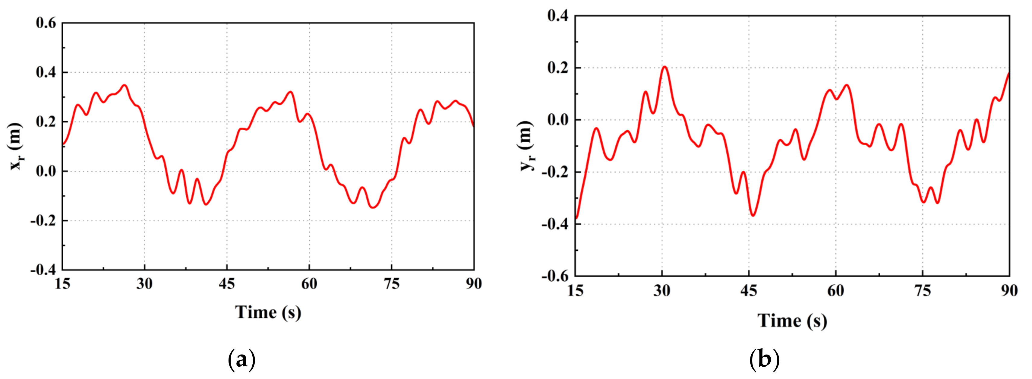
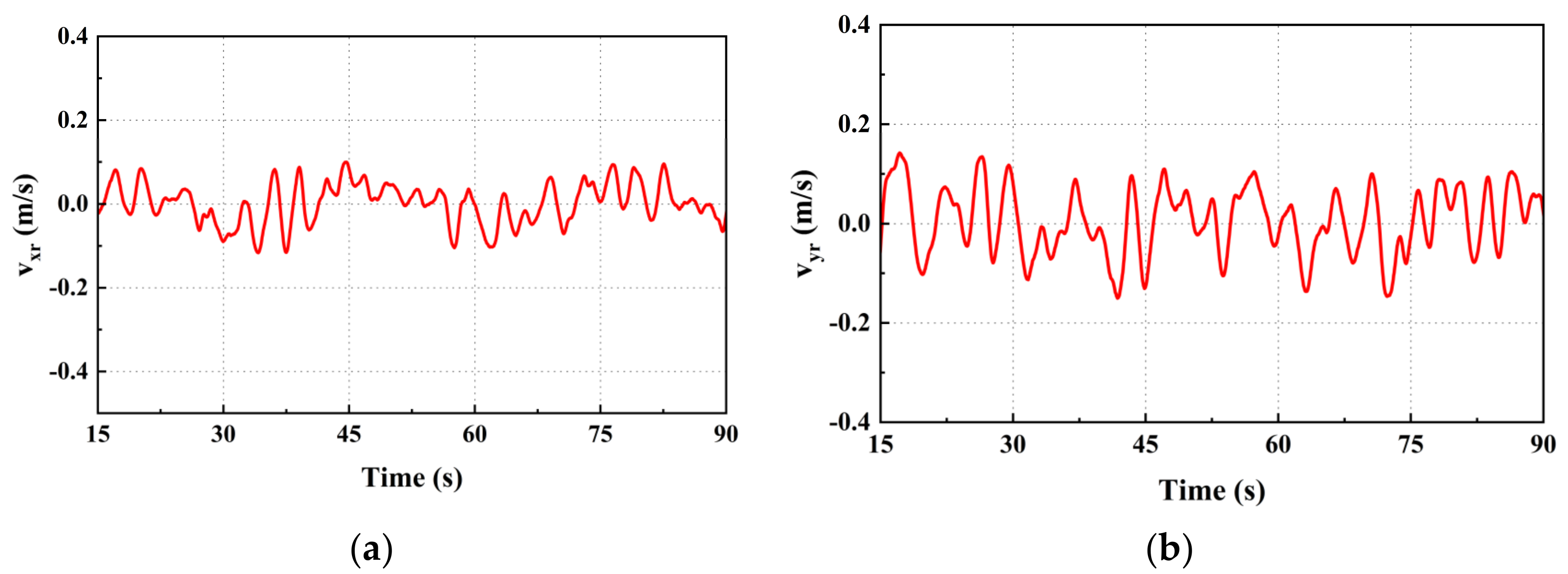
3.1.3. Straight-Sided Ellipse Trajectory

Experiments on the UAV’s tracking of the UGV moving in a straight elliptical trajectory are shown in Figure 19. Since the results of the previous experiments show that the UAV can achieve the tracking of the UGV when it is moving at three speeds, the experiments are conducted only for the UGV moving at speed v1 when the UGV is moving in a straight-sided elliptical trajectory.
We can obtain the position and velocity deviation of the UAV and the UGV when the UGV moves in a straight-sided ellipse with velocity v1 (Figure 20 and Figure 21). The position deviation between the UAV and the UGV in the x- and y-axis directions is always within the range of ±0.4 m, and the speed deviation in the x- and y-axis directions is always within the range of ±0.15 m/s, which indicates that the tracking performance of the UAV for the complex trajectory is still good.

3.2. Landing Experiments

To further verify the landing performance of the UAV, we conducted landing experiments in static and dynamic scenarios (shown in Figure 22). We expect the horizontal landing accuracy to be no more than 0.5 m. In the stationary landmark landing experiment, the UAV ascends to a specific altitude and initiates a tracking landing mission once the landmark enters the field of view of the UGV. To minimize the possibility of error, we replicated three experiments and tabulated the x- and y-axis position coordinates and averaged values from each experiment in Table 9. In the dynamic landing experiment, the UGV moves linearly along the x-axis at three different speeds, while the UAV performs dynamic tracking and landing experiments on the UGV. When the landmark enters the monocular camera’s field of view, the UAV initiates the tracking landing mission. The UAV horizontally approaches the landmark while computing its relative position and altit. Additionally, it adjusts its speed to match that of the UGV. As the UAV reduces its flight altitude, it measures its distance from the center of landmark d. When the relative position of the two meets the landing conditions, the UAV enters the landing mode. During the landing process, it makes sure that the landmark is within the field of view of the monocular camera, while the speed of the UAV is adjusted to ensure that it keeps up with the target during the dynamic landing process. The landmark undergoes decoding measures to obtain information and corner points, followed by the calculation of the relative position between the UAV and the landmark. Based on our pre-experiments, we consider the position and size of the UAV, as well as the requirement to guarantee safety and stability during dynamic landings. When the distance, d, is less than or equal to 0.3 m, the on-board processor will send a command to the UAV flight controller to land and the duty cycle of the PWM will be reduced. The motor will decelerate and the UAV will land on the UGV. Table 10 displays the dynamic landing accuracy of the UAV at three separate vehicle speeds. The results of the experiment indicate that the UAV’s static landing accuracy can achieve a range between 0.03 and 0.04 m. During dynamic landing scenarios, the UAV demonstrated an x-axis landing accuracy of 0.23 m and a y-axis landing accuracy of 0.02 m, which is consistent with the predetermined expectations and satisfies the landing accuracy requirements.

4. Discussion

During the experiment, the UAV was unable to track for an extended period when the UGV was moving at velocity v3. This limitation can be attributed to the low flight altitude of the UAV and site constraints causing the camera to capture an insufficient image, hence increasing the likelihood of loss of the target. In this research, the structural design of the ArUco marker and dimension parameter optimization improved the system’s robustness in recognizing landmarks to some extent. However, it fails to consider the UAV control strategy in situations when the target becomes occluded or is lost for an extended period during the tracking process. Subsequent research can utilize this as a starting point to enhance the system’s ability to identify and track targets with greater accuracy and efficacy.

5. Conclusions

In this paper, we propose a method for tracking and landing UAVs in dynamic environments using nested ArUco markers. Firstly, this study examines tracking and landing as a unified process and proposes a switching strategy for transitioning between tracking and landing modes. Our proposed inner and outer loop controllers, which combine serial PID and fuzzy algorithms, effectively control a quadrotor UAV. Relative position and attitude estimation and landmark recognition detection rely only on vision. Mode conversion of the UAV for dynamic tracking and landing tasks is achieved by calculating the relative positional information between the UAV and the UGV using landmarks. Second, two landmarks with varying sizes were created as nested landmark codes to aid the UAV in tracking and positioning the UGV, taking into account the correlation between ArUco marker size and positioning accuracy. The experiments yielded the optimal landmark size parameters for enhancing the robustness of landmark classification to meet the task requirements. Finally, tracking and landing experiments were conducted at three different speeds. Overall, our adopted method improves the accuracy and robustness of tracking and landing during the dynamic tracking and landing process of UAVs on UGVs with varying motion trajectories. Furthermore, our method demonstrates higher landing accuracy against the dynamic landing platform, providing evidence for its feasibility in dynamic tracking and landing of UAV.

Author Contributions

Conceptualization, H.Z.; Methodology, B.W.; Validation, B.W. and R.M.; Data curation, B.W.; Writing—original draft preparation, B.W. and R.M.; Writing—review and editing, H.Z., T.Y. and Y.S.; Supervision, H.Z.; Project administration, H.Z.; Funding acquisition, H.Z. All authors have read and agreed to the published version of the manuscript.

Funding

This research was funded by the Jilin Province Key R&D Plan Project, grant number 20220202034NC, and the Jilin Provincial Development and Reform Commission Industrial Technology Research and Development Program in 2020, grant number 2020C018-2.

Data Availability Statement

The data used to support the findings of this research are available from the corresponding author upon request.

Conflicts of Interest

The authors declare no conflict of interest.

References

  1. Al-Ghussain, L.; Bailey, S.C.C. Uncrewed Aircraft System Measurements of Atmospheric Surface-Layer Structure during Morning Transition. Bound. -Layer Meteorol. 2022, 185, 229–258. [Google Scholar] [CrossRef]
  2. Greco, R.; Barca, E.; Raumonen, P.; Persia, M.; Tartarino, P. Methodology for measuring dendrometric parameters in a mediterranean forest with UAVs flying inside forest. Int. J. Appl. Earth Obs. Geoinf. 2023, 122, 13. [Google Scholar] [CrossRef]
  3. Abrahams, M.; Sibanda, M.; Dube, T.; Chimonyo, V.G.P.; Mabhaudhi, T. A Systematic Review of UAV Applications for Mapping Neglected and Underutilised Crop Species’ Spatial Distribution and Health. Remote Sens. 2023, 15, 4672. [Google Scholar] [CrossRef]
  4. Sanchez-Lopez, J.L.; Pestana, J.; Saripalli, S.; Campoy, P. An Approach Toward Visual Autonomous Ship Board Landing of a VTOL UAV. J. Intell. Robot. Syst. 2014, 74, 113–127. [Google Scholar] [CrossRef]
  5. Michael, N.; Shen, S.J.; Mohta, K.; Mulgaonkar, Y.; Kumar, V.; Nagatani, K.; Okada, Y.; Kiribayashi, S.; Otake, K.; Yoshida, K.; et al. Collaborative mapping of an earthquake-damaged building via ground and aerial robots. J. Field Robot. 2012, 29, 832–841. [Google Scholar] [CrossRef]
  6. Miki, T.; Khrapchenkov, P.; Hori, K. UAV/UGV Autonomous Cooperation: UAV assists UGV to climb a cliff by attaching a tether. In Proceedings of the IEEE International Conference on Robotics and Automation (ICRA), Montreal, QC, Canada, 20–24 May 2019; IEEE: Piscataway, NJ, USA, 2019; pp. 8041–8047. [Google Scholar]
  7. Sanchez-Lopez, J.L.; Castillo-Lopez, M.; Olivares-Mendez, M.A.; Voos, H. Trajectory Tracking for Aerial Robots: An Optimization-Based Planning and Control Approach. J. Intell. Robot. Syst. 2020, 100, 531–574. [Google Scholar] [CrossRef]
  8. Kassab, M.A.; Maher, A.; Elkazzaz, F.; Zhang, B.C. UAV Target Tracking by Detection via Deep Neural Networks. In Proceedings of the IEEE International Conference on Multimedia and Expo (ICME), Shanghai, China, 8–12 July 2019; IEEE: Piscataway, NJ, USA, 2019; pp. 139–144. [Google Scholar]
  9. Elloumi, M.; Escrig, B.; Dhaou, R.; Idoudi, H.; Saidane, L.A. Designing an energy efficient UAV tracking algorithm. In Proceedings of the 13th International Wireless Communications and Mobile Computing Conference (IWCMC), Valencia, Spain, 26–30 June 2017; IEEE: Piscataway, NJ, USA, 2017; pp. 127–132. [Google Scholar]
  10. Altan, A.; Hacioglu, R. Model predictive control of three-axis gimbal system mounted on UAV for real-time target tracking under external disturbances. Mech. Syst. Signal Proc. 2020, 138, 23. [Google Scholar] [CrossRef]
  11. Jin, S.G.; Zhang, J.Y.; Shen, L.C.; Li, T.X. On-board Vision Autonomous Landing Techniques for Quadrotor: A Survey. In Proceedings of the 35th Chinese Control Conference (CCC), Chengdu, China, 27–29 July 2016; pp. 10284–10289. [Google Scholar]
  12. Nepal, U.; Eslamiat, H. Comparing YOLOv3, YOLOv4 and YOLOv5 for Autonomous Landing Spot Detection in Faulty UAVs. Sensors 2022, 22, 464. [Google Scholar] [CrossRef] [PubMed]
  13. Zhang, H.T.; Hu, B.B.; Xu, Z.C.; Cai, Z.; Liu, B.; Wang, X.D.; Geng, T.; Zhong, S.; Zhao, J. Visual Navigation and Landing Control of an Unmanned Aerial Vehicle on a Moving Autonomous Surface Vehicle via Adaptive Learning. IEEE Trans. Neural Netw. Learn. Syst. 2021, 32, 5345–5355. [Google Scholar] [CrossRef] [PubMed]
  14. Abujoub, S.; McPhee, J.; Westin, C.; Irani, R.A. Unmanned Aerial Vehicle Landing on Maritime Vessels using Signal Prediction of the Ship Motion. In Proceedings of the Conference on OCEANS MTS/IEEE Charleston, Charleston, SC, USA, 22–25 October 2018; IEEE: Piscataway, NJ, USA, 2018. [Google Scholar]
  15. Li, W.Z.; Ge, Y.; Guan, Z.H.; Ye, G. Synchronized Motion-Based UAV-USV Cooperative Autonomous Landing. J. Mar. Sci. Eng. 2022, 10, 1214. [Google Scholar] [CrossRef]
  16. Persson, L.; Muskardin, T.; Wahlberg, B. Cooperative Rendezvous of Ground Vehicle and Aerial Vehicle using Model Predictive Control. In Proceedings of the 56th Annual IEEE Conference on Decision and Control (CDC), Melbourne, Australia, 12–15 December 2017; IEEE: Piscataway, NJ, USA, 2017. [Google Scholar]
  17. Araar, O.; Aouf, N.; Vitanov, I. Vision Based Autonomous Landing of Multirotor UAV on Moving Platform. J. Intell. Robot. Syst. 2017, 85, 369–384. [Google Scholar] [CrossRef]
  18. Borowczyk, A.; Nguyen, D.T.; Nguyen, A.P.V.; Nguyen, D.Q.; Saussié, D.; Le Ny, J. Autonomous Landing of a Multirotor Micro Air Vehicle on a High Velocity Ground Vehicle. In Proceedings of the 20th World Congress of the International-Federation-of-Automatic-Control (IFAC), Toulouse, France, 9–14 July 2017; pp. 10488–10494. [Google Scholar]
  19. Xu, Y.B.; Liu, Z.H.; Wang, X.K. Monocular Vision based Autonomous Landing of Quadrotor through Deep Reinforcement Learning. In Proceedings of the 37th Chinese Control Conference (CCC), Wuhan, China, 25–27 July 2018; pp. 10014–10019. [Google Scholar]
  20. Li, W.J.; Fu, Z.Y. Unmanned aerial vehicle positioning based on multi-sensor information fusion. Geo-Spat. Inf. Sci. 2018, 21, 302–310. [Google Scholar] [CrossRef]
  21. Lim, J.; Lee, T.; Pyo, S.; Lee, J.; Kim, J.; Lee, J. Hemispherical InfraRed (IR) Marker for Reliable Detection for Autonomous Landing on a Moving Ground Vehicle from Various Altitude Angles. IEEE-ASME Trans. Mechatron. 2022, 27, 485–492. [Google Scholar] [CrossRef]
  22. Yuan, B.X.; Ma, W.Y.; Wang, F. High Speed Safe Autonomous Landing Marker Tracking of Fixed Wing Drone Based on Deep Learning. IEEE Access 2022, 10, 80415–80436. [Google Scholar] [CrossRef]
  23. de Croon, G.; Ho, H.W.; De Wagter, C.; van Kampen, E.; Remes, B.; Chu, Q.P. Optic-flow based slope estimation for autonomous landing. Int. J. Micro Air Veh. 2013, 5, 287–297. [Google Scholar] [CrossRef]
  24. Kalaitzakis, M.; Cain, B.; Carroll, S.; Ambrosi, A.; Whitehead, C.; Vitzilaios, N. Fiducial Markers for Pose Estimation: Overview, Applications and Experimental Comparison of the ARTag, AprilTag, ArUco and STag Markers. J. Intell. Robot. Syst. 2021, 101, 26. [Google Scholar] [CrossRef]
Figure 1. UAV visual tracking landing system control strategy.
Drones 07 00703 g001
Figure 2. Mounting positions of the two cameras. The UAV’s center, known as A1, is positioned on the frame’s central axis, 0.18 m above the ground. The coordinates for A1 are set at (0 m, 0 m, 0 m). Meanwhile, the SY011HD camera’s center, A2, is located at (0.08 m, 0 m, 0.06 m).
Drones 07 00703 g002
Figure 3. Control system structure.
Drones 07 00703 g003
Figure 4. Circular trajectory response: (a) circular trajectory tracking; (b) three-axis positional response.
Drones 07 00703 g004
Figure 5. The ArUco markers: (a) outer marker; (b) inner marker.
Drones 07 00703 g005
Figure 6. Parameter optimization experiment: (a) shows the experimental scenario; (b) shows the experimental design.
Drones 07 00703 g006
Figure 7. A tracking landing landmark.
Drones 07 00703 g007
Figure 8. The hardware platform for the tracking and landing system.
Drones 07 00703 g008
Figure 9. The experimental scenario.
Drones 07 00703 g009
Figure 10. Linear reciprocating tracking experimental environment. C1 represents the initial altitude of the UAV while the UGV is in motion at velocity v1. The coordinates of point C1 in space are designated as (0 m, 0 m, 1.0 m). C2 is the initial altitude of the UAV while it travels at velocities v2 and v3. The coordinates of C2 are (0 m, 0 m, 1.2 m). In all three velocity changes, the UGV’s initial coordinates are consistently (−1.1 m, 0 m, 0 m), while the landmark’s initial position is (−1.1 m, 0 m, 0.3 m) due to the landing platform’s height being 0.3 m from the ground.
Drones 07 00703 g010
Figure 11. UAV x-axis position relationship diagram: (a) x-axis absolute position relationship; (b) position deviation in x-axis direction.
Drones 07 00703 g011
Figure 12. UAV y-axis position relationship diagram: (a) y-axis absolute position relationship; (b) position deviation in y-axis direction.
Drones 07 00703 g012
Figure 13. UAV and UGV line speed relationship chart: (a) x-axis velocity relationship; (b) y-axis velocity relationship.
Drones 07 00703 g013
Figure 14. Position relationship between UAV and UGV at three speeds: (a) x-axis position deviation; (b) y-axis position deviation.
Drones 07 00703 g014
Figure 15. Velocity relationship between UAV and UGV at three speeds: (a) x-axis speed deviation; (b) y-axis speed deviation.
Drones 07 00703 g015
Figure 16. Circular trajectory tracking experimental environment. The starting coordinates of the UGV are consistently (0 m, −0.8 m, 0 m). D1 represents the initial altitude of the UAV when the UGV is in motion at speed v1. The coordinates of D1 in space are (0 m, 0 m, 1.0 m). D2 is another initial altitude of the UAV, but this time when the UGV moves at speeds v2 and v3. The coordinates of D2 are (0 m, 0 m, 1.2 m).
Drones 07 00703 g016
Figure 17. Position relationship between UAV and UGV at three speeds: (a) x-axis position deviation; (b) y-axis position deviation.
Drones 07 00703 g017
Figure 18. Velocity relationship between UAV and UGV at three speeds: (a) x-axis speed deviation; (b) y-axis speed deviation.
Drones 07 00703 g018
Figure 19. Straight-sided ellipse trajectory tracking experimental environment. The coordinates of the UAV tracking start point are (0.9 m, −0.6 m, 1.0 m) and the coordinates of the UGV start point are (−0.3 m, −0.6 m, 0 m).
Drones 07 00703 g019
Figure 20. Position deviation of UAV from UGV: (a) x-axis position deviation; (b) y-axis position deviation.
Drones 07 00703 g020
Figure 21. Speed deviation of UAV from UGV: (a) x-axis velocity deviation; (b) y-axis velocity deviation.
Drones 07 00703 g021
Figure 22. UAV landing experiment environment: (a) Static experimental environment; the landmark coordinate point is (0.48 m, 0 m, 0 m) and the UAV start point is (0 m, 0 m, 0 m); (b) dynamic experimental environment; E1 serves as the initial altitude for the UAV when the UGV is traveling at speed v1. The coordinates of E1 in space are (0.0 m, 0.0 m, 1.0 m). On the other hand, when the UGV is moving at speeds v2 and v3, E2 serves as the starting altitude point of the UAV, and its coordinates are (0.0 m, 0.0 m, 1.2 m). It is worth noting that the UGV starting coordinates remain constant at (−1.1 m, 0 m, 0 m) regardless of the speed.
Drones 07 00703 g022
Table 1. Attitude angle and its angular velocity step response metrics.
Attitude ParametersPerformance Indicators
t r (s) t s (s) t p (s) σ (%)
q 0.22 0.27 0.32 3.01
θ 0.400.60 1.53 0.97
p 0.22 0.27 0.32 2.96
ϕ 0.450.60 1.41 0.91
r 0.14 0.18 0.70 0.09
ψ 0.270.40 0.60 1.38
Table 2. Some performance parameters of the cameras.
Parameter TypesPerformance Parameters
SY011HDT265
Active Pixels/frames per second 1920 × 1080 / 30 f p s 848 × 800 / 30 f p s
Angle of vision 130 ° 163 °
Interface typeUSB2.0USB3.1
Table 3. Inner ArUco marker of different sizes’ relative distance estimation data.
Size (mm)Reference Value (mm)Measured Value 1 (mm)Measured Value 2 (mm)Measured Value 3 (mm)Average Value (mm)
20 × 20300306310312309.3
350----
400----
500----
600----
30 × 30300313312311312
350369366368367.7
400426419421422
500----
600----
40 × 40300313311313312.3
350369366371368.7
400426419421423
500524527520523.7
600----
Where “-” indicates that the relative distance could not be calculated because the marker was not detected due to camera resolution issues.
Table 4. Outer ArUco marker of different sizes’ relative distance estimation data.
Size (mm)Reference Value (mm)Measured Value 1 (mm)Measured Value 2 (mm)Measured Value 3 (mm)Average Value (mm)
100 × 100300305306306306
350361360361361
400411412413412
500517518519518
600620623621621
150 × 150300306306306306
350359358358358
400410411410410
500516514515515
600621619620620
200 × 200300307307307307
350359360358359
400410411410410
500515514515515
600619618618618
Table 5. Mean and mean square deviation of the position deviation of UAV from the UGV.
VelocityAverage Value ErrorMean Square Error
x A V E (m/s) y A V E (m/s) x M S E (m/s) y M S E (m/s)
v1 6.73 × 10 2 2.55 × 10 2 7.44 × 10 2 3.08 × 10 2
v2 4.11 × 10 1 8.88 × 10 2 2.75 × 10 1 6.54 × 10 2
Table 6. Mean square sum of velocity deviation of UAV and UGV.
VelocityMean Square Error
v x M S (m/s) v y M S (m/s)
v1 1.30 × 10 2 1.89 × 10 3
v2 1.33 × 10 1 1.32 × 10 2
Table 7. Mean and mean square deviation of the position deviation of UAV from the UGV.
VelocityAverage Value ErrorMean Square Error
x A V E (m/s) y A V E (m/s) x M S E (m/s) y M S E (m/s)
v1 1.65 × 10 1 1.41 × 10 1 1.14 × 10 1 1.02 × 10 1
v2 2.41 × 10 1 2.43 × 10 1 1.35 × 10 1 1.37 × 10 1
Table 8. Mean square sum of velocity deviation of UAV and UGV.
VelocityMean Square Error
v x M S (m/s) v y M S (m/s)
v1 2.89 × 10 3 7.88 × 10 3
v2 7.63 × 10 2 7.55 × 10 2
Table 9. Static landing experiment accuracy and its mean value.
Experimental
Sequence
x-Axis Landing
Accuracy (m)
y-Axis Landing
Accuracy (m)
Test 10.050.04
Test 20.010.04
Test 30.040.05
Average value0.030.04
Table 10. Dynamic landing experiment accuracy and its mean value.
Velocityx-Axis Landing
Accuracy (m)
y-Axis Landing
Accuracy (m)
v10.140.04
v20.230.01
v30.320.01
Average value0.230.02
Disclaimer/Publisher’s Note: The statements, opinions and data contained in all publications are solely those of the individual author(s) and contributor(s) and not of MDPI and/or the editor(s). MDPI and/or the editor(s) disclaim responsibility for any injury to people or property resulting from any ideas, methods, instructions or products referred to in the content.

