Abstract
Fixed-wing, solar-powered unmanned aerial vehicles (SUAVs) can use thermals to expand the duration of flight. Nevertheless, due to the demand for calculating the thermal state parameters of the SUAV during flight, the existing methods still have some shortcomings in their practical applications, such as an inaccurate location estimation of the thermal and an insufficient seeking efficiency. In this paper, by integrating the Gaussian distribution model of thermal updraft of the pitching and roll moment of SUAVs, it is demonstrated that the approach introduced is superior to the traditional methods, disregarding the pitching moment. The simulation indicated that the accuracy and convergence speed of the thermal state estimation, performed while employing the cubature Kalman filter (CKF), are significantly improved after the SUAVs pitching moment is considered. The proposed method improves the automaticity and intelligence of SUAVs autonomous thermal search and enhances the cognitive and decision-making capabilities of SUAVs.
1. Introduction
Unmanned aerial vehicles (UAVs) are widely used in many applications, such as transportation, communication, and target tracking, due to their flexibility, strong adaptability, and low-power consumption [1]. Typically, UAVs can fly automatically without an on-board operator, with a limited payload to accomplish challenging or dangerous missions for human beings, such as humanitarian search and rescue. Nevertheless, general UAVs are powered by batteries, which provide a limited energy capacity, and thus cannot perform long-duration missions [2]. Recently, solar-powered UAVs (SUAVs) have demonstrated greater flight endurance, hence becoming widespread in areas such as communication relays, target tracking, and border surveillance [3,4]. The solar energy harvested by the SUAVs during the daytime covers the electricity demands throughout the day. That is, the SUAV will use the energy stored in the battery overnight, while simultaneously powering and charging during the daytime with the harvested solar energy [5]. Therefore, it is recommended to store additional energy whenever possible, in accordance with the availability of solar energy and battery capacity. A large wingspan is typically adopted for SUAVs for effective energy harvesting, one emerging research area is making SUAVs have the ability to exploit updrafts in the air to increase their flight time [6,7,8].
Based on the study of bird soaring [9], techniques for extracting energy from the atmosphere have been used by humans since the late 1920s [10], such as cross-country flight by manned glider pilots with the localization and utilization of thermal updrafts. Thermals are a special atmospheric phenomenon existing within the low troposphere. There are two main sources of updraft motion: heat caused by the uneven heating of the Earth’s surface by solar radiation, and updrafts along the upwind side of a ridge, cliff, or wave [11]. Exploiting updrafts is considered advantageous for the scenarios that require fixed-wing SUAVs to stay airborne for a long time. The method of utilizing updrafts is straightforward, that is, it uses updrafts to counteract the vertical downward force caused by gravity.
Similar to bird soaring, maximizing the absorption and utilization of thermal updrafts is of great research value for SUAVs. Many investigations have been conducted on exploiting thermal updraft. A method of autonomous soaring to seek the updrafts is proposed in [12], where autonomous thermalling was modeled by a partially observable Markov decision process. A reinforcement learning approach was presented to tackle the task of interthermal cross-country soaring flight in [13]. Therein, the method addresses the decision dilemma between utilizing updrafts while accomplishing the mission objectives. In the case of model-free updrafts, a grid-based thermal mapping approach employing a set of Kalman filters to evaluate the vertical wind speed was utilized [14]. Another approach for a model-free wind field estimation was given in [15]. The above methods enable the mapping of updraft fields without using predefined models. However, we believe that introducing a priori knowledge about the general shape of the thermals may be beneficial for fast localization, especially in the case of limited residence time in a single updraft. After all, the thermal force of the individual updraft field varies over different locations and locating the center of the updraft quickly is essential.
The key to model-based methods is to estimate the center location, the distribution radius, and the center strength of thermal accurately. In [16], using two coupled extended Kalman filters (EKF), the thermal parameter and location estimation was performed. It was found that performing the updates of each of these filters within a loop improved the overall state estimate accuracy. Hazard proposed the unscented Kalman filter (UKF) framework based on the Gaussian thermal model as its measurement and state transaction model, to estimate the thermal state parameters [17]. The simulation result shows that the algorithm is feasible. However, in some special flight path cases, such as straight flight paths, the algorithm in [17] cannot estimate the thermal state parameters as expected, due to inadequate information. Samuel Tabor proposed an autonomous thermal-seeking method, ArduSoar, based on an open-source autopilot software suite, Ardupilot [18]. ArduSoar uses EKF to estimate the state of Gaussian thermal, but its thermal-seeking efficiency is relatively low. In [19], the rolling moment of the SUAV was involved in the measurement and state transition model, and different filter framework such as EKF [20,21], UKF [22,23], and Particle Filter (PF) [24,25,26] were compared in his work. The obtained results in [19] indicate that inducing the roll moment into the measurement model and employing filtering algorithms can effectively estimate the position and strength of the thermal updraft center in time. However, besides the roll moment, the pitching moment of the UAV is also physically relevant to the state information of the thermal updraft. No algorithmic model is available that simultaneously augments both the roll and pitching moment to the thermal updraft measurement model and accomplishes the localization and strength estimation of the updraft using an effective nonlinear filtering algorithm [27].
In this paper, based on the Gaussian distribution model of thermal updraft [28] and the roll moment model proposed by Hazard [19], a pitching moment model of UAVs in a thermal field is proposed. By simultaneously introducing the roll and pitching moment into the thermal updraft measurement model, the UKF and cubature Kalman filter (CKF) [29] algorithms are performed to update the thermal updraft status information instantly.
This paper is structured as follows: The modeling knowledge associated with thermal updrafts and the modeling procedure of the roll and pitching moments of fixed-wing solar UAVs are given in Section 2. In Section 3, after establishing the measurement model proposed in this paper, UKF and CKF algorithms are illustrated. State estimation of the SUAV is accomplished under multiple flight paths in a thermal updraft, and the simulation results and discussion are given in Section 4. A conclusion on the content presented is finally drawn in Section 5.
2. Pitching Dynamics Modeling of SUAV
2.1. Review of Prior Models
Gaussian Thermal Model:
The perception and utilization of thermal is inseparable from the mathematical model of thermal. This study relies on the thermal model proposed by Wharington [28] and modified by Allen [30]. As shown in Figure 1, the and axes in the 3D plot represent the eastward and northward directions of the fixed Earth inertial system, respectively, while the axis represents the thermal updraft velocity. The model is mainly based on three assumptions:
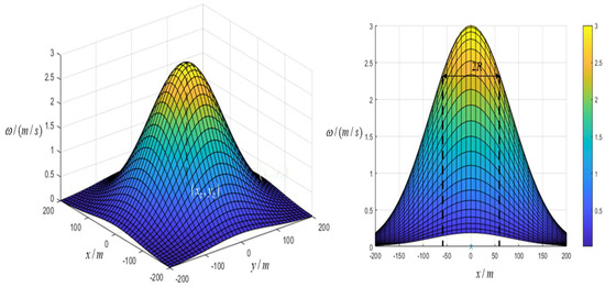
Figure 1.
Three−dimensional and side view of Gaussian thermal updraft model, with .
(1) The state of thermal is stable: the center location, distribution, and vertical wind speed of the thermal do not change in respect to time.
(2) Thermal only has one center and its coordinate position is .
(3) In the same horizon plane, the vertical velocity distribution of thermal updraft is a 2-dimension Gaussian distribution. The maximum vertical velocity of the thermal is (3 m/s). The vertical velocity of the thermal at coordinates is given in Equation (1), where denotes the vertical velocity of the thermal updraft at position , is the peak velocity corresponding to the center of updraft, and represents the radial of thermal strength.
2.2. UAVs Roll Moment Model in Thermal
The UAVs roll moment model is the model [19] that including the SUAVs roll moment in the Gaussian thermal model. As shown in Figure 2, in a typical Gaussian thermal environment, non-uniform upward air velocity around SUAVs can produce a moment for SUAVs pitching axis and roll axis, especially for SUAVs with a large span-chord ratio. The magnitude of the roll and pitching moment have certain physical relations with the thermal state information.
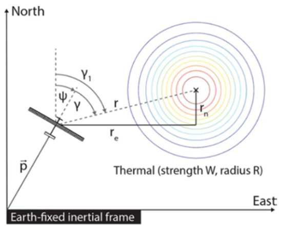
Figure 2.
Relative coordinates and relative heading of aircraft in thermal updraft field.
The relationship between the magnitude of the roll moment and the thermal field is given by Oettershagen [19] as follows:
is the roll moment induced by thermal updraft on the SUAV. is the flat tail lift coefficient. is the air density. is SUAVs air speed. is the chord length of the wing. is the wingspan. is the center strength of the thermal. is the radius of the thermal. and are and coordinates of the thermal center relative to UAV (under the North–East system). is the roll angle of the SUAV, and is the heading angle of the SUAV.
2.3. UAVs Pitching Moment Model in the Thermal
In general, SUAVs center of gravity and its wings aerodynamic center are in the same position, which means that additional lift on UAVs wings does not influence the pitching moment. SUAVs pitching moment in the thermal field is only caused by the non-uniform air velocity distribution on the SUAVs tailplane. Figure 3 shows the uneven distribution of lift force in the thermal field.
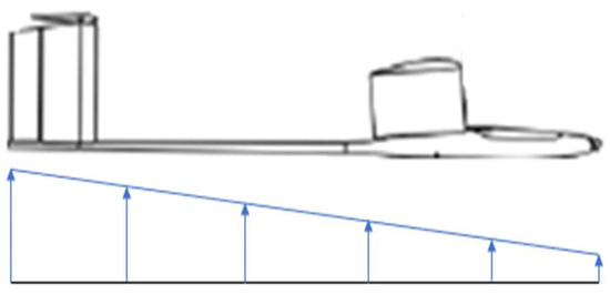
Figure 3.
The uneven distribution of the updraft in the thermal updraft field along the fuselage axis.
The pitching moment of SUAVs on the pitching axis in the thermal field can be obtained by multiplying additional lift force on the flat tail by the flat tail moment arm:
where is the area of the flat tail, and is the moment arm of the flat tail (that is, the distance from the aerodynamic center to the gravity center of SUAV). is the updraft difference between the tail’s aerodynamic center and the SUAVs center of gravity, calculated by (4). Other parameters own the same meaning as Equation (2).
The gradient of the updraft distribution along SUAVs fuselage axis is:
By substituting Equations (4) and (5) into Equation (3), the pitching moment of the SUAV in the thermal field can be deduced as:
3. State Estimation Algorithms
3.1. Thermal State Estimation and Measurement Models
In Section 2, the mathematical models of the thermal and roll moment of the fixed-wing SUAV in the thermal are introduced. However, thermal model still needs to be adapted into appropriate time-update and measurement-update equations for facilitating the application of the state estimation. Given the thermal model in Equation (1), the thermal state can be represented as:
Consider the single thermal updraft model described by the system state estimation equation
and the measurement model
where is the discrete-time index, and represents the measurement vector. Process noise and measurement noise are given by and , respectively, as zero-mean white noise with known distributions. The three measurement variables in (9) are obtained by Equations (1), (2) and (6). By augmenting the roll and pitching moments of a fixed-wing UAV into the thermal updraft state model with the given prior knowledge, the accurate localization and strength analysis of the center of the thermal updraft is fundamentally a state estimation process. Within the state estimation problem based on known models, filtering algorithms are favored owing to their superiority in rapidity and accuracy. There are many available filter frameworks, such as the EKF, UKF and PF. Each of these frameworks has its own advantages and disadvantages. In order to control the variables, we use the UKF and CKF framework in this study.
3.2. Unscented Kalman Filter
UKF combines unscented transform (UT) with the Kalman filter. The basic idea of UT is to approximate a Gaussian distribution with sigma points (where is the dimension of the state vector). That is, to replace the approximation of the nonlinear function by an approximation of the probability density distribution of nonlinear functions. This feature determines that UKF is only applicable to Gaussian noise systems. Since UKF does not linearize the nonlinear function and ignore its higher-order terms, the estimates of the mean and variance are more accurate than those by EKF [27]. Next, UKF and CKF algorithms are introduced based on the following model for convenience.
Here, and are the state and measurement vectors. and are the process and measurement noises. The underlying idea of the filter based on Gaussian assumption is to derive the posterior distribution of states by Gaussian approximation, namely:
The main steps of the UKF algorithm are as follows:
Prediction:
- 1.
- Calculating sigma points:
In which, and are a scale factor. decides the distribution of the sigma points around . Generally, is a small positive number (), and the value of is .
- 2.
- Time update:
In which
The value of is two under the Gaussian distribution [23].
Update:
- Calculating sigma points:
- Measurement update:
- State Estimation:
3.3. Cubature Kalman Filter
The cubature Kalman filter (CKF) [29] is also a commonly used nonlinear filtering algorithm, which can be obtained by only using volume points instead of integrating points. The specific process can be summarized as follows.
Prediction:
- Calculating sigma point:
- Time update:
Updating:
- Calculating sigma point:
- Measurement update:
- State Estimation:
4. Simulation Results Analysis
In order to verify the effectiveness of the new model, a simulation system was established. In the simulation, the efficiency and accuracy of the UKF and CKF estimations with different measurement and state transition models were compared.
4.1. The Algorithm Efficiency
The simulation is mainly used to compare the improvements of the efficiency and accuracy of the filter after considering the pitching moment in the algorithm. First of all, a single Gaussian thermal was generated in the simulation. Next, the initial flight position of the aircraft was selected, and a straight flight path was set for the SUAV to fly through the thermal. Then, the data generated by the simulation, such as the UAV position, attitude, roll moment value, pitching moment value in the thermal field, and the thermal’s vertical speed at the corresponding location, are inputted into the algorithm to estimate the state of the thermal. Finally, the history of the filter estimation outcomes is recorded. The parameters of the simulation experiment were set as shown in Table 1.

Table 1.
Simulation experiment parameters.
Figure 4 depicts the history of thermal center location estimation for UKF prediction using different prior models. Figure 5 then gives the corresponding error and variance of the UKF estimates of the state and position of the thermal updraft. It is evident that the tracking accuracy of the thermal rise center is effectively improved by adding the pitching moment to the measurement models. Figure 6 shows the thermal tracking process of the CKF under different measurement models. The corresponding estimated accuracy and variance are given in Figure 7. Figure 5a and Figure 7a show that the accuracy of state estimation, especially the accuracy of position estimation, increases with the quantity of data points. The rapid decrease in the residuals after considering the pitch moment implies that incorporating the pitch moment into the measurement models is meaningful for the thermal tracking algorithm.
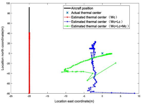
Figure 4.
Estimating history of thermal location under UKF.
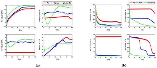
Figure 5.
(a) State estimation residual history under different prior model under UKF; and (b) state estimation variance history under different prior model under UKF.
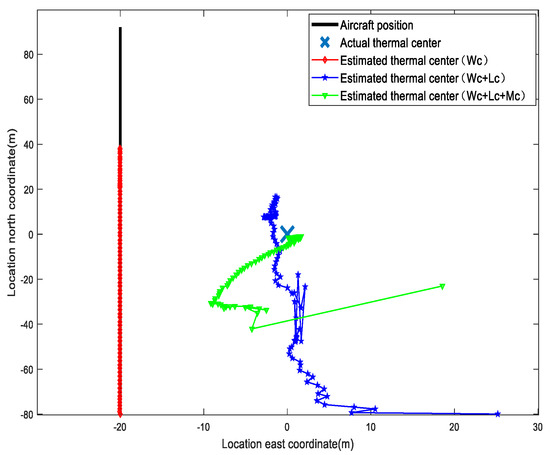
Figure 6.
Estimating history of thermal location under CKF.
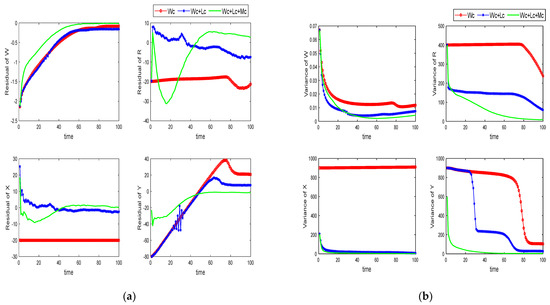
Figure 7.
(a) State estimation residual history under different prior model under CKF; and (b) state estimation variance history under different prior model under CKF.
Figure 5b and Figure 7b both depict that after including the pitching moment in the measurement model, the estimated results converge quicker than the model, which only considers the Gaussian thermal model and SUAVs roll moment in the thermal. It means that the new algorithm can make SUAVs tracking thermal more efficiently. In addition, on the straight flight path, if the measurement model only includes the Gaussian thermal model and roll moment, the algorithm may not have enough information to accurately estimate the coordinates of the thermal.
In this flight mode, taking the three-dimensional measurement information as an example, the comparison of the residual errors of the estimated results of the UKF and CKF on the thermal updraft is shown in Figure 8. It can be seen from the figure that the estimation effect of CKF is slightly better than that of UKF.
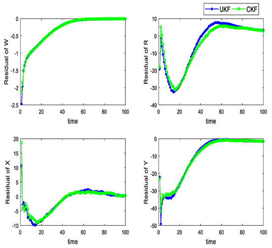
Figure 8.
Comparison chart of UKF and CKF residuals.
In addition to the residual and variance comparison plots of the estimation results, the root mean square error (RMSE), a widespread algorithm evaluation metric, is also adopted here as a criterion to measure the improvement.
where is the estimated value corresponding to the true state at time in the simulation run .The simulation is performed for a total of runs, each run containing time steps. As shown in Table 2, the average RMSE (ARMSE) of the UKF and CKF for 100 time steps over 100 simulation runs are given, where 1D, 2D, and 3D denote the dimensionality of the measurement model, respectively. The mean runtimes of the two algorithms are given in Table 3.
Table 2.
Comparison of ARMSEs of UKF and CKF under different measurement models.
Table 3.
Comparison of runtimes of UKF and CKF under different measurement models.
4.2. The Algorithm Efficiency under Different Flight Paths
In order to verify that under different flight paths the efficiency and accuracy of the new algorithm still improved, different flight paths were set in the simulation to compare the convergence of the parameter residuals and variance.
A special flight path, which directly passed through the center of the thermal, was set in the comparison. As shown in Figure 9, the thermal center location estimation histories are predicted by UKF and CKF. Figure 10a,c indicates the parameters of residual history under three different measurement models. It can be found that under this flight path, the thermal coordinates estimation’s residual converges quickly. All of the parameters are estimable, since the coordinate of the thermal center is the initial state estimation. From Figure 10b,d, the thermal coordinates confidence interval does not convergence, which means that the accurate estimation of the thermal center is a coincidence. Similar conclusions can be drawn from the quantitative analysis in Table 4.
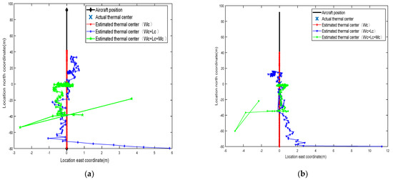
Figure 9.
(a) Estimating history of thermal location in the new flight path under UKF; and (b) estimating history of thermal location in the new flight path under CKF.
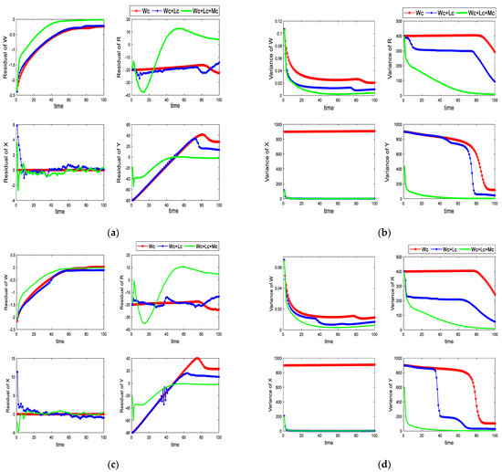
Figure 10.
(a) State estimation residual history under different prior model in the new flight path under UKF; (b) state estimation variance history under different prior model in the new flight path under UKF; (c) state estimation residual history under different prior model in the new flight path under CKF; and (d) state estimation variance history under different prior model in the new flight Path under CKF.
Table 4.
Comparison of ARMSEs of UKF and CKF under different measurement models.
Similarly, the comparison of the residual error of the estimation results of the UKF and CKF on the thermal updraft under the three-dimensional measurement model is shown in Figure 11.
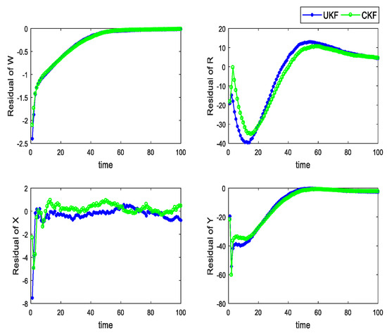
Figure 11.
Comparison chart of UKF and CKF residuals.
4.3. The Algorithm Efficiency While Hovering around the Thermal
The actual process of SUAVs utilizing the thermal is to locate the thermal center while hovering around the thermal. When SUAVs detect that the intensity of vertical air velocity reaches a certain threshold, the state estimation algorithm will be turned on and the SUAVs will be controlled to hover around the thermal center with a specific hover radius. In order to verify the effect of the new model in the actual thermal-seeking process, we built SUAVs heading control in the simulation to control SUAVs hovering around the thermal during the thermal state estimating process. Figure 12a–d demonstrates the convergence of the residuals and variance of the state estimation results with a time migration. Figure 13a,b shows the SUAVs flight trajectory and the thermal coordinate estimation history under a different measurement model. Table 5 shows the time cost for the algorithms under different conditions. Consistent with the preceding, the ARMSE values of the state estimation of 100 cycles of the UKF and CKF running with 100 time steps are each provided in Table 6.
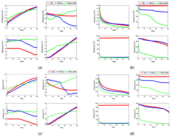
Figure 12.
(a) State estimation residual history under different prior model while hovering around the thermal under UKF; (b) state estimation variance history under different prior model while hovering around the thermal under UKF; (c) state estimation residual history under different prior model while hovering around the thermal under CKF; and (d) state estimation variance history under different prior model while hovering around the thermal under CKF.
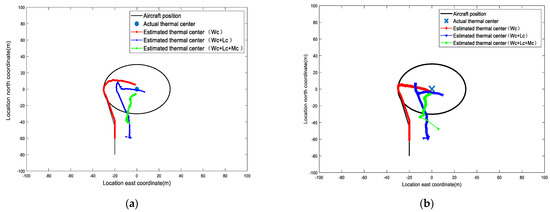
Figure 13.
(a) Estimating history of thermal location while hovering around the thermal under UKF; and (b) estimating history of thermal location while hovering around the thermal under CKF.
Table 5.
Comparison of runtimes of UKF and CKF under different measurement models.
Table 6.
Comparison of ARMSEs of UKF and CKF under different measurement models.
Similarly, the comparison of the residual error of the estimation results of the UKF and CKF on the thermal updraft is shown in Figure 14. The results show that both UKF and CKF can accurately estimate the state of the thermal updraft, while CKF is more stable. From the above results, it is easy to see that while the SUAVs are flying around the thermal updraft, although the SUAVs can eventually achieve accurate localization under all three measurement models, the 3D measurement model can identify the shortest path to the center, which ultimately reflects the best convergence and accuracy in the results of state estimation. From the quantitative analysis in Table 6, the accuracy of the 3D measurement system in evaluating the location of the thermal center is improved by 80% compared to the 1D measurement system, and by 60% compared to the 2D system Therefore, it is feasible and necessary to augment the pitching moment to the measurement model. This is of practicable value for elongating the endurance of the solar UAV. As for the nonlinear state estimation, both the UKF and CKF show great superiority, with CKF proving its stability.
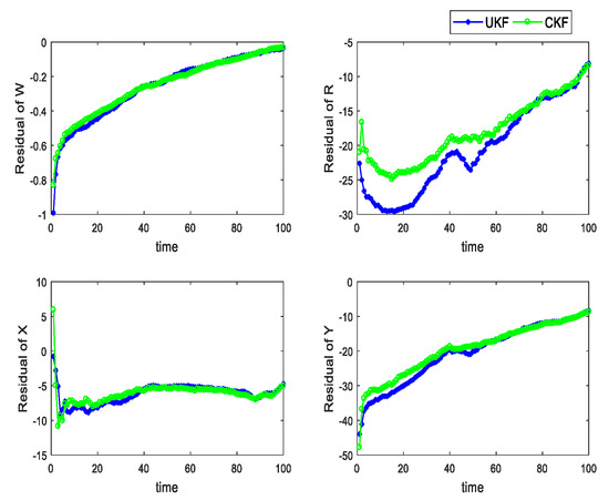
Figure 14.
Comparison chart of UKF and CKF residuals.
5. Conclusions
In this paper, based on the Gaussian thermal model, the pitching moment model of fixed-wing SUAVs in thermals is proposed. The model allows SUAVs to estimate the thermal online. Simulation experiments show that after introducing the SUAVs pitching moment into the system measurement model, the convergence speed of the algorithm and the accuracy of the thermal center positioning are greatly improved. Since the algorithm is tested by the flight simulation data of a real SUAV model, the algorithm can effectively improve the search efficiency of the thermal in the real experiment. This paper only describes the method of improving the SUAVs thermal-seeking efficiency by improving the prior model. Regardless of whether it is in the framework of the CKF or UKF state estimation, the introduction of the pitching moment can improve the UAVs perception and utilization of thermal updraft to a certain extent.
Since state estimation algorithms and SUAVs flight strategy are also important factors that limit the thermal-seeking efficiency, some additional extensions can be conducted in these fields to increase the UAVs cognition and decision-making ability in the future.
Author Contributions
Conceptualization and methodology, K.L. (Ke Li 1) and X.C.; software, K.L. (Ke Li 1) and X.C.; validation, S.W., K.L. (Ke Li 2) and H.L.; writing—review and editing, X.C. and H.L.; supervision, K.L. (Ke Li 1) and B.L.; project administration, K.L. (Ke Li 1); funding acquisition, K.L. (Ke Li 1) All authors have read and agreed to the published version of the manuscript.
Funding
This work is supported by the National Natural Science Foundation of China (No. 61773039) and (No. 20XXJCJQXX1045).
Data Availability Statement
Not applicable.
Conflicts of Interest
The authors declare no conflict of interest.
References
- Gupta, S.G.; Ghonge MM, P.M.; Jawandhiya, P. Review of Unmanned Aircraft System (UAS). Int. J. Adv. Res. Comput. Eng. Technol. 2013. [Google Scholar] [CrossRef]
- Lun, Y.; Wang, H.; Wu, J.; Liu, Y.; Wang, Y. Target Search in Dynamic Environments With Multiple Solar-Powered UAVs. IEEE Trans. Veh. Technol. 2022, 71, 9309–9321. [Google Scholar] [CrossRef]
- Tian, Z.; Haas, Z.J.; Shinde, S. Routing in Solar-Powered UAV Delivery System. Drones 2022, 6, 282. [Google Scholar] [CrossRef]
- Chu, Y.; Ho, C.; Lee, Y.; Li, B. Development of a Solar-Powered Unmanned Aerial Vehicle for Extended Flight Endurance. Drones 2021, 5, 44. [Google Scholar] [CrossRef]
- El-Atab, N.; Mishra, R.B.; Alshanbari, R.; Hussain, M.M. Solar Powered Small Unmanned Aerial Vehicles: A Review. Energy Technology 2021, 9, 2170121. [Google Scholar] [CrossRef]
- Kim, E.J.; Perez, R.E. Neuroevolutionary Control for Autonomous Soaring. Aerospace 2021, 8, 267. [Google Scholar] [CrossRef]
- Huang, Y.; Chen, J.; Wang, H.; Su, G. A method of 3D path planning for solar-powered UAV with fixed target and solar tracking. Aerosp. Sci. Technol. 2019, 92, 831–838. [Google Scholar] [CrossRef]
- Reddy, G.; Celani, A.; Sejnowski, T.J.; Vergassola, M. Learning to soar in turbulent environments. Proc. Natl. Acad. Sci. USA 2016, 113, E4877–E4884. [Google Scholar] [CrossRef]
- Mohamed, A.; Taylor, G.K.; Watkins, S.; Windsor, S.P. Opportunistic soaring by birds suggests new opportunities for atmospheric energy harvesting by flying robots. J. R. Soc. Interface 2022, 19, 20220671. [Google Scholar] [CrossRef]
- Notter, S.; Groß, P.; Schrapel, P.; Fichter, W. Multiple Thermal Updraft Estimation and Observability Analysis. J. Guid. Control Dyn. 2020, 43, 490–503. [Google Scholar] [CrossRef]
- Allen, M.J. Autonomous Soaring for Small Unmanned Aerial Vehicles (UAVs). 2006. Available online: https://xueshu.baidu.com/usercenter/paper/show?paperid=1y2w0xb0w44q0my0652j00d0rw780327 (accessed on 17 January 2023).
- Guilliard, I.; Rogahn, R.; Piavis, J.; Kolobov, A. Autonomous Thermalling as a Partially Observable Markov Decision Process. In Proceedings of the 14th Conference on Robotics—Science and Systems, Pittsburgh, PA, USA, 26–30 June 2018. [Google Scholar]
- Notter, S.; Zürn, M.; Groß, P.; Fichter, W. Reinforced Learning to Cross-Country Soar in the Vertical Plane of Motion. In Proceedings of the AIAA Scitech 2019 Forum, San Diego, CA, USA, 7–11 January 2019. [Google Scholar]
- Cheng, K.; Langelaan, J.W. Guided Exploration for Coordinated Autonomous Soaring Flight. In Proceedings of the AIAA Guidance, Navigation, and Control Conference, National Harbor, MD, USA, 13–17 January 2014. [Google Scholar]
- Lawrance NR, J.; Sukkarieh, S. Path Planning for Autonomous Soaring Flightin Dynamic Wind Fields. In Proceedings of the IEEE International Conference on Robotics and Automation (ICRA), Shanghai, China, 9–13 May 2011. [Google Scholar]
- Kahn, A.D. Atmospheric Thermal Location Estimation. J. Guid. Control Dyn. 2017, 40, 2359–2365. [Google Scholar] [CrossRef]
- Hazard, M. Unscented Kalman Filter for Thermal Parameter Identification. In Proceedings of the 48th AIAA Aerospace Sciences Meeting Including the New Horizons Forum and Aerospace Exposition, Orlando, FL, USA, 4–7 January 2010. [Google Scholar]
- Tabor, S.; Guilliard, I.; Kolobov, A. ArduSoar: An Open-Source Thermalling Controller for Resource-Constrained Autopilots. In Proceedings of the 25th IEEE/RSJ International Conference on Intelligent Robots and Systems (IROS), Madrid, Spain, 1–5 October 2018. [Google Scholar]
- Oettershagen, P.; Stastny, T.; Hinzmann, T.; Rudin, K.; Mantel, T.; Melzer, A.; Wawrzacz, B.; Hitz, G.; Siegwart, R. Robotic technologies for solar-powered UAVs: Fully autonomous updraft-aware aerial sensing for multiday search-and-rescue missions. J. Field Robot. 2018, 35, 612–640. [Google Scholar] [CrossRef]
- Meng, Y.; Wang, W.; Han, H.; Ban, J. A visual/inertial integrated landing guidance method for UAV landing on the ship. Aerosp. Sci. Technol. 2019, 85, 474–480. [Google Scholar] [CrossRef]
- Song, H.-L.; Ko, Y.-C. Robust and Low Complexity Beam Tracking With Monopulse Signal for UAV Communications. Ieee Trans. Veh. Technol. 2021, 70, 3505–3513. [Google Scholar] [CrossRef]
- Guo, K.; Ye, Z.; Liu, D.; Peng, X. UAV flight control sensing enhancement with a data-driven adaptive fusion model. Reliab. Eng. Syst. Saf. 2021, 213, 107654. [Google Scholar] [CrossRef]
- Julier, S.; Uhlmann, J.; Durrant-Whyte, H.F. A new method for the nonlinear transformation of means and covariances in filters and estimators. IEEE Trans. Autom. Control 2000, 45, 477–482. [Google Scholar] [CrossRef]
- Djuric, P.M.; Kotecha, J.H.; Zhang, J.; Huang, Y.; Ghirmai, T.; Bugallo, M.F.; Miguez, J. Particle filtering. IEEE Signal Process. Mag. 2003, 20, 19–38. [Google Scholar] [CrossRef]
- Santos, N.P.; Lobo, V.; Bernardino, A. Unscented Particle Filters with Refinement Steps for UAV Pose Tracking. J. Intell. Robot. Syst. 2021, 102, 52. [Google Scholar] [CrossRef]
- Fu, R.; Al-Absi, M.A.; Lee, Y.S.; Al-Absi, A.A.; Lee, H.J. Modified Uncertainty Error Aware Estimation Model for Tracking the Path of Unmanned Aerial Vehicles. Appl. Sci. 2022, 12, 11313. [Google Scholar] [CrossRef]
- Lefebvre, T.; Bruyninckx, H.; De Schutter, J. Kalman filters for non-linear systems: A comparison of performance. Int J Control 2004, 77, 639–653. [Google Scholar] [CrossRef]
- Edwards, D. Implementation Details and Flight Test Results of an Autonomous Soaring Controller; In Proceedings of the 46 th AIAA Guidance, Navigation and Control Conference and Exhibit, Reno, Nevada, 7–10 January 2008.
- Arasaratnam, I.; Haykin, S. Cubature Kalman Filters. IEEE Trans Autom Control 2009, 54, 1254–1269. [Google Scholar] [CrossRef]
- Allen, M. Updraft Model for Development of Autonomous Soaring Uninhabited Air Vehicles. In Proceedings of the 44th AIAA Aerospace Sciences Meeting and Exhibit, Reno, Nevada, 9–12 January 2006. [Google Scholar]


Disclaimer/Publisher’s Note: The statements, opinions and data contained in all publications are solely those of the individual author(s) and contributor(s) and not of MDPI and/or the editor(s). MDPI and/or the editor(s) disclaim responsibility for any injury to people or property resulting from any ideas, methods, instructions or products referred to in the content. |
© 2023 by the authors. Licensee MDPI, Basel, Switzerland. This article is an open access article distributed under the terms and conditions of the Creative Commons Attribution (CC BY) license (https://creativecommons.org/licenses/by/4.0/).