Object Detection-Based System for Traffic Signs on Drone-Captured Images

Abstract

The construction industry is on the path to digital transformation. One of the main challenges in this process is inspecting, assessing, and maintaining civil infrastructures and construction elements. However, Artificial Intelligence (AI) and Unmanned Aerial Vehicles (UAVs) can support the tedious and time-consuming work inspection processes. This article presents an innovative object detection-based system which enables the detection and geo-referencing of different traffic signs from RGB images captured by a drone’s onboard camera, thus improving the realization of road element inventories in civil infrastructures. The computer vision component follows the typical methodology for a deep-learning-based SW: dataset creation, election and training of the most accurate object detection model, and testing. The result is the creation of a new dataset with a wider variety of traffic signs and an object detection-based system using Faster R-CNN to enable the detection and geo-location of traffic signs from drone-captured images. Despite some significant challenges, such as the lack of drone-captured images with labeled traffic signs and the imbalance in the number of images for traffic signal detection, the computer vision component allows for the accurate detection of traffic signs from UAV images.

1. Introduction

Unmanned Aircraft Vehicles (UAV), commonly referred to as drones, can perform aerial operations that manned aircraft find challenging. Using drones offers considerable economic savings and benefits for the environment, and at the same time, it reduces human life risks. Currently, some factors limit drone-based services and product innovation [1]:

• Increasing dependence on poorly interoperable proprietary technologies.
• The risk that they entail for people, other vehicles, and property.

Additionally, the potential applications for drones, especially those in manned areas or non-segregated airspace, are only possible by developing and validating certain key enabling technologies. The development and integration of these technologies require the drone to be equipped with sophisticated sensors to have a precise knowledge of the environment (perception), trusted communication capabilities (identification, availability, and cyber-security), and the ability to make intelligent decisions autonomously in real-time to react to unforeseen situations (detect and avoid, safe coordination, and contingency). The embedded architecture of drones shares limitations with most computer-embedded systems: limited space, limited power resources, increasing computation requirements, the complexity of the applications, time-to-market requirements, etc. [2].

These issues have a massive impact on the European innovation framework. Hence, there needs to be support for the initiatives that bring globally harmonized, commercially exploitable, and widely accessible R&D ecosystems. One of these initiatives is the H2020-ECSEL-2018 project named Comp4Drones [3] which aims to provide a framework of key enabling technologies for safe and autonomous drones. This project focuses on safe software and hardware drone architectures and deals with a holistically designed ecosystem, ranging from the application to electronic components, realized as a tightly integrated multi-vendor and compositional drone-embedded architecture solution and a toolchain complementing the compositional architecture principles.

Within the scope of the Comp4Drones project, an object detection-based system emerges as a key enabling technology for payload data analytics to address one of the main challenges in the construction industry, that is, the inspection, assessment, and maintenance of civil infrastructures and construction elements. Today, a specialized workforce is in charge of performing visual inspections and making the corresponding inventories. This work is a tiresome and time-consuming task prone to human errors, and therefore, an expensive job, so accelerating the process is crucial. Therefore, the construction industry is on the path to digital transformation by widely incorporating the BIM (building information modeling) concept in the civil works environment. Additionally, current trends in Artificial Intelligence (AI) and Unmanned Aerial Vehicles (UAVs) can support a smart inspection process, using low-cost drones, RGB cameras, automated detection algorithms, and remote operations [4]. With this in consideration, this article presents an innovative object detection-based system which enables the detection and geo-referencing of different traffic signs from RGB images captured by the drones’ onboard camera, improving the realization of the road element inventories in any civil infrastructure or construction elements.

2. Related Work

Object detection is a computer vision technique that detects instances of semantic objects of a particular class inside a picture, indicating object position and object class via a bounding box description. In this respect, the results of AlexNet’s performance in the 2012 ImageNet Challenge [5] encouraged using deep learning methods alongside Convolutional Neural Networks (CNN) for computer vision issues. As a result, all current techniques for object detection are deep learning-based, and they use CNNs to carry out this detection.

CNN-based object detectors have recently led to a significant improvement in the performance and efficiency of object detection techniques, thanks to fundamental advances in both deep learning algorithms and high-quality annotated datasets. Related to such datasets, some of the most prominent in the field include PASCAL VOC [6], MSCOCO [7], ImageNet [8], and DOTA [9].

CNN-based object detectors are divided into two main frameworks: one-stage algorithms and two-stage algorithms. The first group usually includes models based on You Only Look Once (YOLO) [10] or a Single Shot MultiBox Detector (SSD) [11], which employ an object classifier and regression in a dense manner without using a region proposal; while the second group includes models such as Faster Region-based CNN (R-CNN) [12] or a Region-based Fully Convolutional Network (R-FCN) [13], which extracts region proposals followed by classification and regression.

The two-stage detection method has often been used and is still a powerful paradigm. In this case, the first stage creates Regions of Interest (RoI, or object proposals), and then in the second stage, bounding box regression is used to categorize and locate the objects. The region proposal stage is skipped during the one-stage detection; instead, direct classification and localization of the bounding boxes are performed. Two-stage algorithms provide the highest detection accuracy, although they are frequently slower. Due to the several inference steps required for each image, the performance (frames per second) is not as good as that of one-stage detectors.

The most important two-stage object detection algorithms are based on the Region-CNN (R-CNN) family [14]. The R-CNN is one of the most sophisticated CNN-based deep learning object detection techniques. The Fast R-CNN [15] and Faster R-CNN have evolved algorithms for faster object detection than R-CNN, as well as other advancements such as Mask R-CNN [16] and the most recent development, Granulated R-CNN (G-RCNN) [17].

Nevertheless, state-of-the-art object detection models that achieve promising performance in natural scene datasets, such as PASCAL VOC or MSCOCO, usually exhibit unsatisfactory results on UAV images. For example, mainstream detectors such as Cascade R-CNN or CornerNet showed a strong performance in an empirical study carried out in 2018 on the MSCOCO dataset, achieving APs of 42.8% and 40.6%, respectively [18]. However, these good metrics dropped off significantly when these models were evaluated in UAV-specialized datasets such as VisDrone [19]. In the VisDrone Challenge of 2019, the previous models Cascade R-CNN and CornerNet only achieved APs of 16.09% and 17.41%, respectively [20].

This cross-domain gap between standard images (e.g., MSCOCO or PASCAL VOC) and UAV images may be ascribed to the following factors [19,21,22]:

• Small object detection. Objects are usually small in size in UAV images, and deep neural networks based on convolution kernels usually overlook or heavily compress small objects’ intrinsic features and patterns, especially when the images have a high resolution.
• Occlusion. The objects are generally occluded by other objects or background obstacles in drone-based scenes.
• Large-scale variations. The objects usually have a significant variation in scale, even for objects of the same class.
• Viewpoint variation. Since the dataset contains images captured from a top-view angle, while other images might be captured from a lower-view angle, the features learned from the object at different angles are not transferable in principle.

Different techniques have been also created to fix the challenges mentioned above. A common solution is to split the high-resolution image into small uniform crops and apply the object detection model on each one. Still, the problem is the computational increase involved in processing each part. In connection, other techniques emerged to optimize the cropping of images. For example, using the Density-Map guided object detection Network (DMNet) [23] provides guidance for cropping images based statistically on an object density map of an image. Another way is the use of pyramid networks or FPN [24] since they improve the detection accuracy by fusing high-level and low-level features.

Alternatively, one of the most important ways to achieve greater accuracy in UAV images is by creating high-quality annotated datasets specialized in this type of imagery. Mittal et al. [21] made a compilation of some of the most prominent datasets in this field, such as VEDAI [25], UAV-BD [26], and VisDrone [19]. However, creating new datasets with a wider variety of objects is still necessary, as many of these datasets focus on vehicle detection.

Regarding Traffic Sign Detection (TSD) or road sign detection, the first solutions used classic machine learning techniques such as SVM [27], but currently, deep learning is being used and performs remarkably well. Nowadays, TSD is very important in developing autonomous vehicles and Automated Driver Assistance Systems (ADAS), so the models are specialized in images of the traffic signs for terrestrial vehicles [28,29]. Amongst other solutions, Tabernik et al. [30] used a modified Mask R-CNN to detect 200 traffic signals in a new large signal dataset, while Shen et al. [31] implemented spatial pyramid pooling (SPP) to boost YOLOv3 [32], and detected the four Taiwan prohibitory signs. More recently, other scientific articles have emerged, such as detection using the multi-scale attention pyramid network [33] or improved Faster R-CNN [34]. However, TSD from UAV has yet to have as many studies conducted as compared to TSD from terrestrial vehicles. The study by Houben et al. [35] showed that it may be possible to use YOLOv2 in UAV videos, and Ertler et al. [36] used UAV images for road traffic elements detection using YOLOv4.

Below,

Table 1. Summary of object detection models and their potential application to TSD using UAV images/videos.

Object Detection Model				Traffic Sign Detection (TSD)	UAV Images/Videos
- Fast +	+ Accuracy -	One-stage algorithms	YOLO
			SSD		X
			YOLOv2	X	X
			YOLOv4
		Two-stage algorithms	R-CNN
			Fast R-CNN
			Faster R-CNN	X	X
			Mask R-CNN	X
			G-RCNN
			Cascade R-CNN
			CornetNet

summarizes all the above-mentioned object detection models and their potential application to TSD using UAV images or videos, ranked from less to more accuracy and more to less speed.

Therefore, this article goes beyond the existing related works by adopting a two-stage model based on the Region-CNN (R-CNN) family [14], working over UAV images for TSD, while proposing a new and high-quality annotated dataset, given that it is one of the most important ways to improve the accuracy of the object detection models.

3. Proposed Solution

The proposed object detection-based system is a computer vision component based on previously-trained CNN algorithms, able to automatically detect and geo-reference different traffic signs from RGB images captured by the drones’ onboard camera.

This computer vision component follows the typical methodology for a deep-learning-based SW: first, the dataset creation; then, the election and training of the most accurate object detection model; and finally, testing of the trained object detection model. Based on this, Figure 1 shows the conceptual implementation diagram of the computer vision component, leading to the following sub-sections.

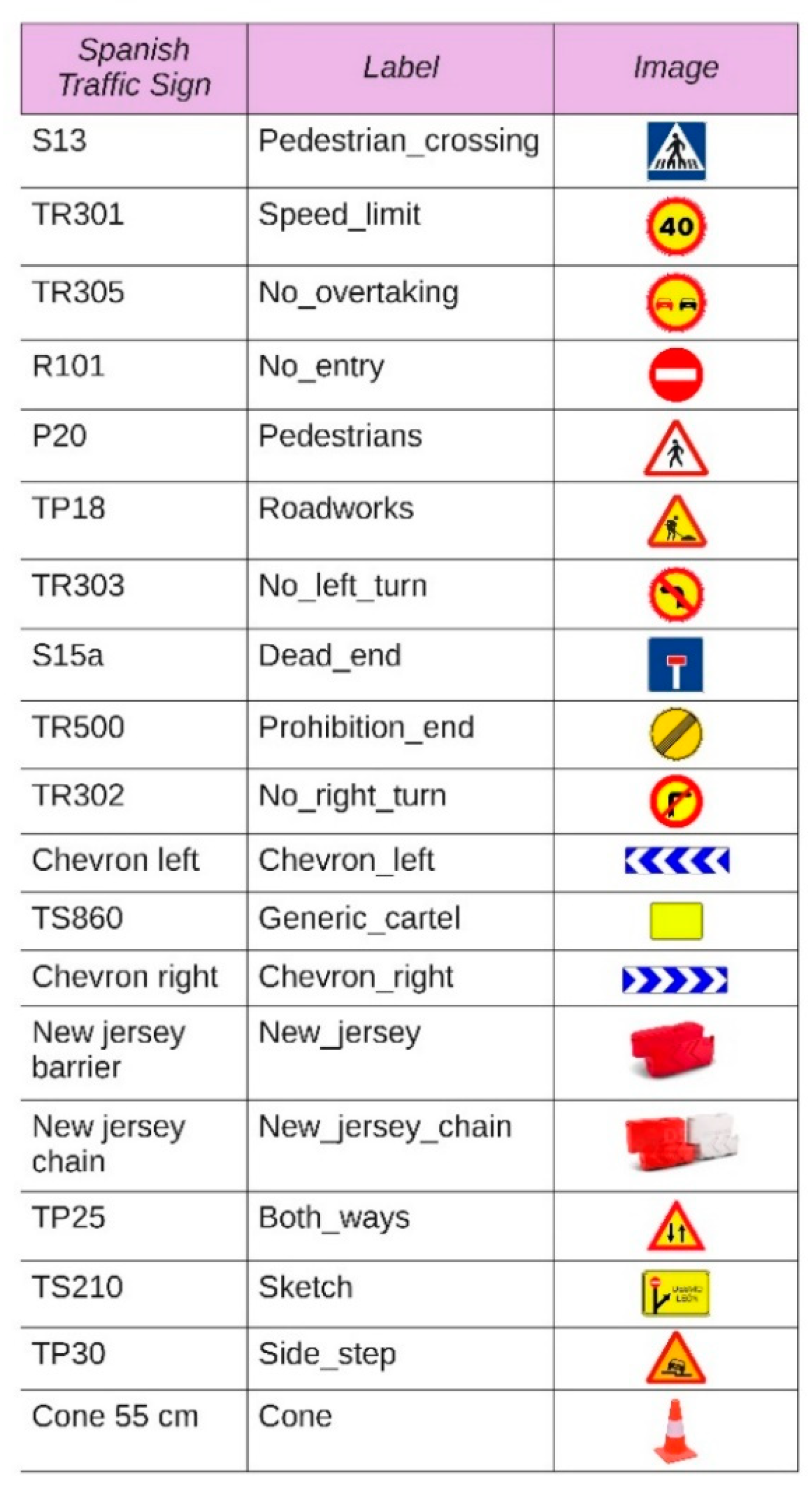
3.1. Dataset Collection

Following state-of-the-art techniques and based on the artificial intelligence methodology, one of the critical steps in achieving greater accuracy for object detection algorithms, in this case, is the creation of high-quality annotated datasets in UAV images. As stated in this particular case, there are a few labeled image datasets for traffic signal detection with a UAV view, so creating new datasets with a wider variety of traffic signs is necessary.

In the first attempt, datasets contained traffic signs with a frontal view. However, due to the change of view between a chopped plane and a frontal plane, it was necessary to perform a preliminary study to see if a model trained with this type of image could be extrapolated to images captured with UAVs. For this purpose, the German Traffic Sign Detection Benchmark (GTSDB) dataset [37] was used. The GTSDB dataset contains an excellent set of images labeled for detection, although with a minimal number of categories, as described in Section 3.1.1. This study allowed for discarding drone flight altitudes and pitch angles of the UAV camera since the models trained with frontal view images were not extrapolated to images of these configurations. Specifically, flights were tested with configurations of 12, 15, 20, 30, and 45 m of flight altitude and with 35, 45, 50, and 90 degrees of camera pitch. After the study, it was concluded that the valid flights were those with altitudes between 12 and 20 m and angles between 35° and 50°, including the limits in both cases.

Once the analysis’ feasibility was confirmed with the available data, a dataset with the largest number of images of the requested classes was built, according to the description in Section 3.1.6. For most of the classes, it was sufficient to select the suitable ones from the datasets mentioned in Section 3.1.2, however in some special categories, such as “cone” and “new-jersey”, the lack of data was solved utilizing simulation techniques with Unreal Engine and AirSim, as detailed in Section 3.1.3.

Considering this methodology, the following subsections describe the process for the Comp4Drones dataset creation.

3.1.1. Dataset for Preliminary Study

The German Traffic Sign Detection Benchmark (GTSDB) was presented at the International Joint Conference on Neural Networks (IJCNN) 2013 [37]. It is a dataset composed of 900 images (600 for training and 300 for testing), divided into four categories, “prohibitory”, “danger”, “mandatory”, and “other”.

This dataset has helped to perform the preliminary study of the behavior of models trained with images of street and road signs from the frontal view, applied in the detection of images obtained by UAVs with images taken at different heights and different camera tilt angles.

3.1.2. Datasets Used

The Mapillary Traffic Sign Dataset [38] is the world’s largest and most diverse publicly available traffic sign dataset. With 401 classes of traffic signs and more than 50,000 manually annotated images, trained machines can detect and recognize traffic signs. It has approximately 300,000 tags, where the most frequent class is “other sign”. After analyzing the classes, it was possible to use from the complete dataset, 6289 images with a total of 11 classes and 8986 labels.

The Belgium traffic sign dataset [39] contains more than 210 assigned categories in 9006 images and 13,480 labeled signs. After studying the data, we found that only 14 categories of the original dataset could be used, leaving 1729 images with 1852 labels for the project. Of these 14 categories, only 10 had labeled signals useful for the detection model.

The Russian Traffic Sign Dataset [40], comprises 179,138 images with 198 signal categories and 104,358 labels. From this set, after performing the exploratory analysis of the data, it was seen that for our project, a total of 33,736 labels could be used in a total of 22,401 images with 14 categories. Therefore, this dataset is the main dataset of the project, since it is the one that contributes the most images and tags to the final set used for training, contributing 70% of the images and 77% of the tags.

The DFG Slovenian Traffic Sign Dataset [30] contains more than 200 assigned categories in 6957 images and 14,208 labeled signals. After studying the data, it was found that only 12 categories from the original dataset, resulting in 1369 images with 1549 labels, could be used for the project.

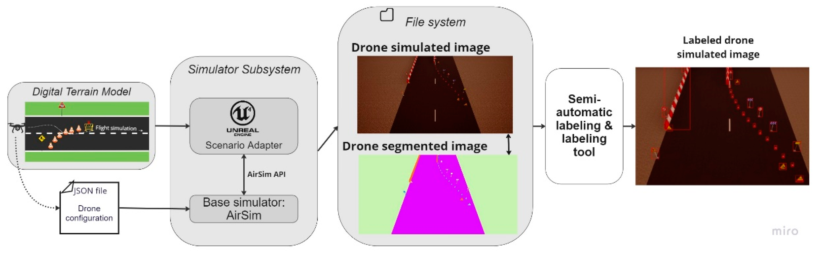
3.1.3. Videos Generated with AirSim (Drone Simulation Environment)

Due to the lack of data in some of the project classes, such as “cone” and “new_jersey”, we decided to work with the simulation alternative to cover this gap in the data. For that purpose, the Unreal Engine tool was used to generate road environments with traffic signs. Then, these environments were included in the AirSim [41] simulator to obtain simulated UAV flight videos and flight images in both RGB and segmented images (which has helped in the labeling work, allowing a semi-automation of the same). Figure 2 shows the labeling process:

In order to have a wide variety of simulated scenarios, simulated flights under different degrees of luminosity were performed. Therefore, different levels of variability of the same scenarios in different periods of the day were obtained. The result is the generation of 52 images and the inclusion of 240 traffic sign labels based on the environments and traffic sign simulation models provided for the Comp4Drones project. Figure 3 shows the trained model’s performance under three simulations with different luminosity levels.

3.1.4. Images from Drone Flight Videos

Under the scope of the Comp4Drones European project [4], in the Flight Test Centre ATLAS (Villacarrillo, Jaén, Spain), a data collection campaign was performed in the real environment to build a dataset with real drone-captured images. ATLAS counts with 1.000 Km² of segregated airspace until 5.000 ft. available jointly with a main runaway of 600 m and an auxiliary one of 400 m allowed for performing long-range flights even with the current Spanish UAS regulations. The drone used for the flight replicates the Matrice600 platform from DJI: an off-the-shelf multi-rotor platform with a 5 Kg payload, around 20 minutes of endurance, and a very versatile configuration since it has enough space to integrate the different sensors and equipment, in this case, an RGB camera.

In more detail, to construct the dataset, the drones performed nine flights at different heights and angles along a road with different types of signals, collecting more than 4500 images that we compiled for testing purposes.

Table 2. Summary of images captured during the data collection campaign.

Flight No.	Images Captured	Height	Degrees	Direction
1	533	20 m	45°	Railway
2	591	20 m	45°	Parallel to railway
3	234	30 m	Zenithal	Railway
4	511	20 m	35°	Railway
5	596	20 m	35°	Parallel to railway
6	573	20 m	50°	Railway
7	530	20 m	50°	Parallel to railway
8	437	12 m	45°	Railway
9	525	15 m	45°	Zig zag

summarizes the number of images captured for each flight that will be used to train the computer vision component.

Figure 4 shows an example of the images captured from the drone during the data collection campaign in Spain.

3.1.5. Cones Dataset

To work on the detection of cones, three different specific datasets were analyzed: the Traffic Cone Image Dataset [42] with 263 images, compiled for testing purposes and labeled by hand; the Duckietown Object Detection Dataset [43] with 1956 images of only three classes, from which 372 have cone annotations; and the Real-time Traffic Cones Detection For Automatic Racing [44], similar to the first one, with 544 images, fully annotated.

A closer look at Figure 5 shows that the types of images available in these datasets do not fit with the rest of the traffic signal datasets. Therefore, these datasets do not help improve the model in detecting the cone element since they cause undesired results and unrealistic detections, as can be seen in Figure 6.

To solve this problem and to cover the lack of “cone” images captured from a drone, it was decided to generate some simulated environments and perform the labeling. For this reason, very few “cone” elements are available in the dataset.

3.1.6. Dataset Used in Training

For each of the selected datasets, an exploratory study of the data was conducted to filter and choose the categories that match those desired for the project, preventing the use of the entire dataset in any of the cases. In Figure 7, all the traffic signs used are compiled, including their label and an example image. Figure 8 shows the number of samples available for each class and considers the merged dataset. Note that, at this point, for the “new_jersey”, “new_jersey_chain”, and “cone” classes, only simulated images were used, and for the rest of the classes, only real images were considered.

A total of 31,841 images with 46,363 labels, split 90–10% between the training and test sets were employed.

Table 3. Data distribution of the traffic sign classes in the training and test sets.

Traffic Sign Class	Train	Test
Pedestrian_crossing	24,189	2687
Speed_limit	9279	1137
No_overtaking	2037	263
No_entry	1374	167
Pedestrians	1305	160
Roadworks	1280	169
No_left_turn	416	47
Dead_end	367	41
Prohibition_end	270	34
No_right_turn	170	22
Chevron_left	141	20
Generic_cartel	139	15
Chevron_right	107	19
New_jersey	102	16
New_jersey_chain	92	14
Both_ways	94	10
Sketch	85	9
Side_step	63	7
Cone	14	2

shows the final distribution of these two sets. In the distribution plots, the data are very unbalanced between the most represented classes, “pedestrian_crossing” or “speed_limit”, and the least represented classes, “cone” and “side_step”. It is important to bear this fact in mind as it will accentuate the model results’ differences.

3.2. Election and Training of the Object Detection Model

As mentioned in Section 2, many generations arose regarding the R-CNN family [10,14]. These generations generally outperform their predecessors in efficiency, test execution time, and performance. Regardless, these networks usually require several phases [45]:

• A region proposal algorithm is used to create bounding boxes or locations of potential objects in the image. In the R-CNN architecture, it is an algorithm such as Edge Boxes.
• A feature generation stage is used to gather information about these objects’ features, so a CNN is generally used.
• A final stage of final classification determines the object’s class.
• A regression layer is used to improve the accuracy of the object’s bounding box coordinates.

Specifically, Faster R-CNN [12], the successor of R-CNN and Fast R-CNN [15], is an object detection network first published in 2015 that proposes the use of a new module for the region proposal algorithm, that is, a Region Proposal Network (RPN). This new module shares convolutional features with the detection network, improving efficiency and detection. This RPN is trained end-to-end to generate good object candidates, and then it uses Fast R-CNN as a detection network to generate the final predictions. In other words, it is a new detection mechanism in which the RPN tells Fast R-CNN where to look. Figure 9 shows the general architecture of the Faster R-CNN model.

Therefore, the choice of the Faster R-CNN detection model for this work is motivated by the fact that it has been a widely-implemented model in the industry since its publication, with a performance that made it state-of-the-art at its inception. Given its wide use, many machine learning frameworks have included this model in their libraries or via API (for example, PyTorch [46] or TensorFlow [47]), facilitating its study and implementation. There are also several implementations based on this model within the field of aerial image object detection, such as [48,49,50].

More specifically, the RPN takes an image of any size as input and returns a set of object proposals and an “objectness” score for each that indicates a measure of belonging to an object or the background. In our case, RPN proposes new traffic signal regions. For this, a CNN is used as a backbone, for example, VGG-16 [51]. In this case, 13 convolutional layers are shared between the CNN backbones of the detection and proposition components. The feature map output by the last shared convolutional layer is scanned with a 3 × 3 spatial window to obtain the proposed regions, which then forms a mini-network that generates a smaller feature delivered to two siblings fully connected layers: a box regression layer (reg) and a box classification layer (cls). Multiple proposed regions are predicted at each position of the sliding window, with a maximum of k propositions. Therefore, if the bounding box is coded as four coordinates (two corners) and the classification into two scores (two-class softmax and object or background), the reg layer has four k outputs with the k boxes coordinates and the cls layer has two k scores, indicating the probability of being an object, for each proposal. The number k parameterizes different sizes and aspect ratios, called anchors. Each anchor is associated with a specific size and aspect ratio, by default k = 9 is used with three size scales (small, medium, and large, depending on the area in pixels) and three aspect ratios (1:1, 1:2, and 2:1). In Figure 10, we can see the idea behind the anchors and how they are visualized in the input image.

Complementarily, Fast R-CNN is the detector network in the Faster R-CNN architecture. The Fast R-CNN does not define the CNN backbone or how the Region of Interest (RoI) is achieved, since the RPN is used as the region proposal algorithm and the same CNN backbone is used for both components. Fast R-CNN consists of a CNN that generates a feature map, a new layer called RoI pooling, and some fully connected layers finished with two sibling output layers: one for the object classification and another for regression to refine bounding boxes. In our case, Fast R-CNN predicts the type of traffic sign.

The training of the proposed object detection model with the Faster R-CNN architecture was carried out with the Object Detection Tensorflow API [47], applying a configuration with 19 classes, an input size of 640 × 640, an InceptionRestnetV2 from Keras used as feature extractor, an anchor configuration with the following: scale {0.25, 0.5, 1.0, 2.0}, aspect_ratios {0.5, 1.0, 2.0}, height_stride of 16, width_stride of 16, a batch_size of 2, and momentum optimized with a value of 0.9, and data augmentation applying changes only in saturation, contrast, and hue. A server with an AMD Ryzen 9 3900X 12-Core CPU, 32 GB of RAM, and an NVIDIA GeForce RTX 3090 GPU was used for the training, and the environment configuration was carried out in a Docker container with Python 3.8.10 and the TensorFlow 2.9.2 framework.

It is essential to know that the drone images have dimensions of 5472 × 3648 pixels and that the model input is 640 × 640, so image pre-processing was performed in different sizes with iterative cropping to avoid losing detections of medium or small elements. Such an iterative cropping process consists of analyzing the whole image, dividing the image in two and analyzing each of the halves, dividing the entire image in four and analyzing the four parts, and so on until the entire image has been divided into sixteen pieces. To rebuild the results as single detections of each element of the image, non_max_suppression was applied on all the bounding boxes detected in relation to the original image’s dimensions.

3.3. Geolocation of Detected Traffic Signs

Once the Faster R-CNN network works on the traffic signs’ detection and position according to the image pixels, it uses the drone geo-localization to seek the traffic signs’ geo-localization. To calculate the traffic signs’ geo-localization, the method from the study “Detection, tracking, and geolocation of moving vehicle from UAV using monocular camera” [52] was followed. For the calculations, a series of data provided by the drone is required, such as the geolocation of the drone in latitude, longitude, and altitude, and camera parameters such as the angles and focal length. Figure 11 shows a schema of the calculations:

This study [52] shows the steps to obtain the latitude and longitude coordinates of the detected traffic sign from the UAV’s geographical position, which receives images and information from the lens used as the focal length. The following items summarize the process:

• Establish the transformation formula of the pixel coordinate frame to the East-North-Up (ENU) frame through the camera frame. For this purpose, the rotation of the ENU frame matrix of the drone camera is calculated. The position of the drone in ENU frame values is obtained.
• Calculate the position of the signal in the image using the image size and the bounding box.
• Finally, calculate the target signal’s depth and the target’s latitude and longitude in terms of the target position in the ENU frame. Transform the ENU frame coordinates into the World Geodetic System (GPS coordinates).

In this case, fourteen data parameters for the geo-location calculation are used which can be divided into camera and drone-related data such as the pitch, roll, yaw, and focal length of the camera as well as the latitude, longitude, and height of the drone when taking the image. Reference data for the calculation, such as the latitude, longitude, and reference altitude, are taken at the starting point of the drone flight as well as data obtained from the object-detection model, such as the X and Y position of the detected element and width and height of the analyzed image.

4. Results and Discussion

As a result, the proposed object detection-based system enables the detection and geo-referencing of different traffic signs from drone-captured images with the final purpose of accelerating the realization of road element inventories carried out in the inspection, assessment, and maintenance of civil infrastructures. The system outputs a CSV file that lists all detected traffic signs over the test images, indicating the type of traffic sign, the classification score, and the geo-localization in cartesian and geographic coordinates. Figure 12 shows how this computer vision component is used in the application scenario proposed within the Comp4Drones project.

The following subsections describe the performance of the computer vision component quantitatively through evaluation metrics, as well as qualitatively through several examples of detection on different types of images.

4.1. Evaluation of the Object Detection Model

4.1.1. Evaluation Metrics

The mean Average Precision (mAP) is currently the primary metric used for object detection, though its definition changes depending on the dataset or criteria being studied [53]. It is, therefore, necessary to clarify the following concepts in order to comprehend this metric:

• Precision (P): is the ratio of True Positive (TP) detections to all positive detections, including False Positives (FP).
• $P = \frac{TP}{TP + FP}$
• Recall (R): is the ratio of True Positive (TP) detections to all real positives, including those that were not detected, that is, False Negatives (FN).
• $R = \frac{TP}{TP + FN}$
• Precision/recall curve (p(r)): is produced by combining the two previous metrics. The precision-recall curve helps to select the best threshold that maximizes both precision and recall.
• IoU (Intersection over Union): is a metric that measures the degree to which the real boundary box, which is frequently manually labeled, and the predicted boundary box overlap, as it is shown in Figure 13. This is the parameter used to establish a threshold to discriminate between a false positive and a true positive prediction (0 there is no overlap, 1 there is full overlap).

Figure 13. Calculation of the intersection over union.

Figure 13. Calculation of the intersection over union.

Considering these four measurements, the Average Precision (AP) can be calculated according to PASCAL VOC [6], either via interpolation for challenges,

$$AP \approx \frac{1}{11}{\sum }_{r \in \left\{0,0.1,\dots ,1\right\}}^{ }{p}_{interp}\left(r\right), \mathrm{where} p_{interp}\left(r\right) = \underset{r_r\ge r}{\max }p\left(r_r\right),$$

or as the area under the precision/recall curve (AUC),

$$AP = {\oint }_0^{1}p\left(r\right) dr, \mathrm{where} p\left(r\right) \mathrm{is} \mathrm{the} \mathrm{precision}/\mathrm{recall} \mathrm{curve},$$

and also approximated by the following formula,

$$AP = {\sum }_{ }^{ }\left(r_{n+1} -r_n\right) p_{interp}\left(r_{n+1}\right), \mathrm{where} p_{interp}\left(r_{n+1}\right) = \underset{r_r\ge r_{n+1}}{\max }p\left(r_r\right).$$

Finally, the mAP is calculated using the averaged AP of all classes. If the IoU threshold is equal to 0.5, this is the mAP for the PASCAL-VOC Challenge 2010+ criteria. The higher this score, the more accurate the model is.

For the evaluation of the proposed CNN-based object detection system, the framework proposed in MSCOCO [7] was used. They perform a slight modification in this metric and do not distinguish between AP and mAP, simply computing an average AP over all the categories and different IoU values which include AP, ${\mathrm{AP}}^{50}$(refer to the average precision calculated for the set IoU level of 0.5), and ${\mathrm{AP}}^{75}$ (IoU threshold of 0.75) metrics. Then, the AP is computed by averaging all 10 IoU thresholds (i.e., in the range {0.50:0.95}, with the uniform step size 0.05) of all categories, which is subsequently used as the main metric for ranking. In addition, the MSCOCO evaluation proposes to calculate the AP (averaging the 10 IoU thresholds) across three object scales: small (object area <${32}^2$ pixels), medium (${32}^2$ < area < ${96}^2$), and large (area > ${96}^2$) objects.

4.1.2. Evaluation with the New Dataset under PASCAL-VOC Challenge 2010+ Criteria

This section presents the model’s results in the new dataset of various traffic sign datasets, simulated images, and real drone-captured images. After training the model with 90% of the dataset images, the remaining 10% are evaluated according to the PASCAL-VOC Challenge 2010+ criteria. As a reminder, this criterion indicates the AP of each class using an IoU of 0.5. The results can be seen in

Table 4. Evaluation using PASCAL-VOC Challenge 2010+ criteria of the test dataset.

Traffic Sign Class	Average Precision (AP) %	Mean Average Precision (mAP) %
New_jersey_chain	95.03	56.30
Pedestrian_crossing	93.55
No_overtaking	89.49
No_entry	88.58
Prohibition_end	81.50
Pedestrians	80.16
Sketch	79.76
Speed_limit	78.55
Side_step	71.79
No_left_turn	70.75
Dead_end	68.08
Roadworks	60.66
No_right_turn	42.70
Chevron_left	37.77
Chevron_right	23.79
New_jersey	3.90
Both_ways	3.65
Generic_cartel	0.00
Cone	0

.

The best possible AP would be 100%, meaning that the model can identify all positive examples (i.e., traffic signs) without making false negatives. However, the mAP of 56.3% is an acceptable value in terms of the signal detection models’ performance, referencing other works, such as [22], in which the maximum mAP was 45.4%. In any case, the AP value is a complex measure that depends to a large extent on the problem, dataset, etc. It is more important to compare different detection models evaluating the same dataset or to be able to compare the relative performances between classes, as in our case.

More specifically, there are large differences in performance among classes due to an unbalanced dataset. There is a strong correlation between the number of images in the dataset and the consequential trained and the obtained AP. Except for “new_jersey_chain”, which is a simulated class, the class that is best detected by far is “pedestrian_crossing”, which is the class with the most samples in the training set, with more than 24,000, much higher “speed_limit” (9000), “no_overtaking” (2000), and the rest of the traffic signs. In addition, it must be added that it is a very different signal from the rest of the classes; it is a square blue signal (there are only two such classes) with a triangle in the middle, which improves detection and classification rates. For example, “no_overtaking” and “no_entry” also had excellent AP values due to being one of the most sampled classes. On the other hand, “speed_limit”, despite being the second class with the most samples, had a good AP, but not one of the best. This may be because it is a round signal and similar to many classes of the dataset, generating many false positives in the model.

Regarding classes with few training and test samples, the “sketch” and “side_step” signals stand out as good. Despite being two of the classes with fewer samples, they have an AP greater than 70%, although, in the same way, the test results are not very significant given the small size of the test sample of only nine and seven signals, respectively. On the other hand, other signals with few samples, such as “both_ways” or “generic_cartel”, were not practically detected in the few test images.

The effect of the number of classes on training is demonstrated in the case of signals that are the same but symmetrical, such as those of “no_turn” and “chevron”. These classes differ only between the right and left, and there is a higher AP in those with more data samples. In the case of “no_left_turn”, which has more than twice as many samples as its right counterpart, its AP is 70.75% versus 42.70% for the right. The same happens with the “chevron” classes, the left has about 30% more samples and its AP is 37.77%, compared to 23.79% for the right. However, both values are lower than average due to the number of training samples.

Regarding the simulated classes, “new_jersey_chain” stands out with the absolute best AP of 95.03%. This score may be because the model can detect all the New Jersey generated with the simulated drone images. However, the performance with the real ones is unknown, as there are no real images available captured from drones. At the same time, this makes the detection of an individual “new_jersey” practically null, with an AP lower than 4%, probably because it classifies them as a chain. Regarding the cones, no detection was obtained on the two cones that were in the test; since there are only fourteen simulated training ones, it is clear that the model did not learn to detect cones.

In conclusion, due to the large differences between the number of samples in the training set, a good AP was obtained for the classes with more training data. Still, these results are hindered by the model’s poor performance in those classes with few or simulated data. This fact means that the model has learned to detect about 10 classes out of the 19 total well. Furthermore, given the small number of test objects, some results may not be statistically significant.

4.1.3. Evaluation with the New Dataset under Microsoft COCO 2016 Challenge Criteria

In this case, the same results are evaluated as before but using the MSCOCO 2016 Challenge criteria. As mentioned, it shows the AP (equivalent to PASCAL’s mAP) for various IoU thresholds and object sizes.

Table 5. Evaluation using Microsoft COCO 2016 Challenge criteria of the test dataset.

Average Precision Type	Area Size	Average Precision (AP) %
$A{P}^{IoU=.50:0.05:.95}$ or AP	All	43.8
$A{P}^{50}$	All	60.5
$A{P}^{75}$	All	51.8
$A{P}^S$	Small	30.6
$A{P}^M$	Medium	47.3
$A{P}^L$	Large	66.4

shows the results obtained in the test set.

These results show that the $A{P}^{50}$ is 60.5%, very close to its PASCAL-VOC mAP equivalent. As expected, the $A{P}^{75}$drops to 51.8% as detection becomes more demanding by asking for a higher minimum IoU. With the AP, the same thing happens, going down to 43.8% due to the greater requirement. These are expected results that show that the model can detect accurately to a greater extent.

Regarding the AP, according to the object’s size, the importance of the size of the traffic sign in the image for its detection is observed. The large-size signals are detected with a good AP of 66.4%, while those with small size are only detected with an AP of 30.6%. Since the dataset is made up of frontal images obtained from cars, this effect with images obtained from UAVs should increase. Therefore, to reduce this effect, the real images obtained from the drone are cut to obtain better detection.

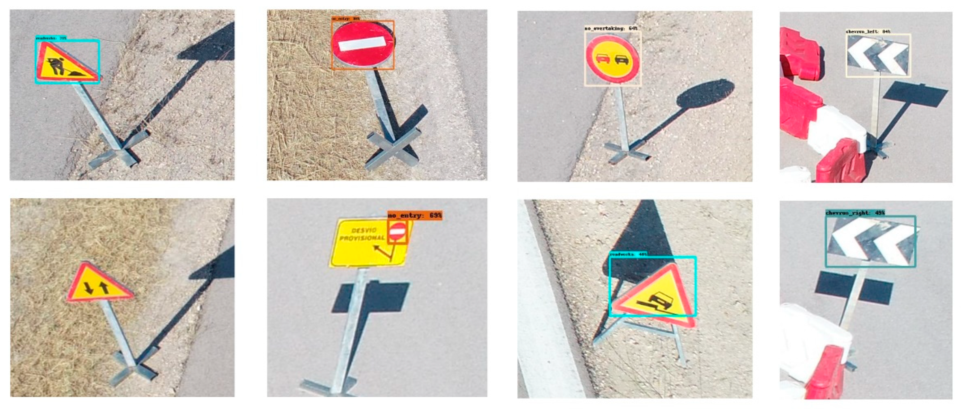
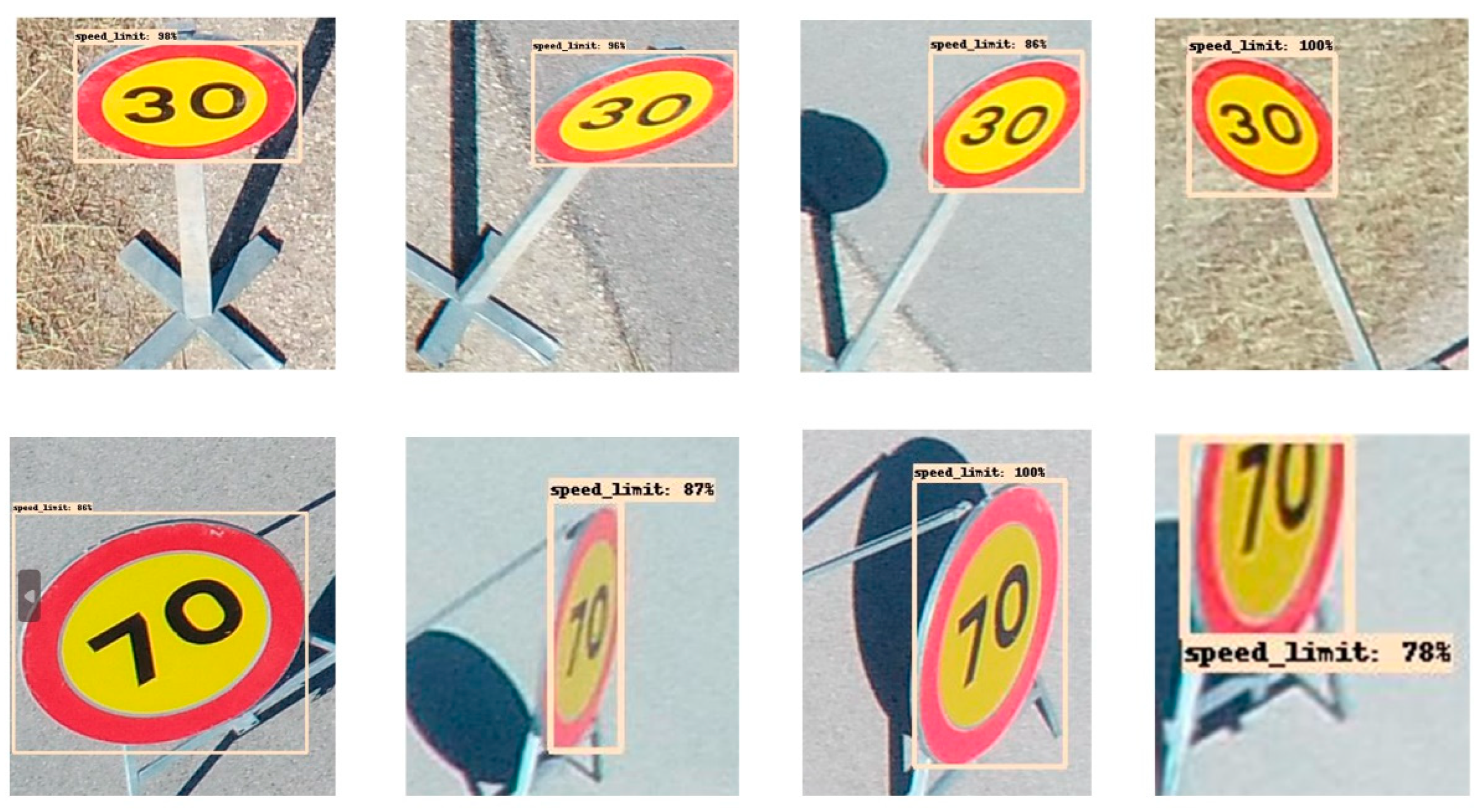
4.2. Detection Results

This section gathers the model’s results while detecting traffic signs on real and simulated drone images. It is important to note that on the one hand, the simulated drone images are labeled and are different from the ones used for training. On the other hand, the real drone images captured during the data collection campaign are not labeled.

4.2.1. Detections on Images from Videos Generated by Drone Simulation Environment

Given the lack of real images from drones for the detection of the required traffic signs, a test of the model is made over a series of videos generated with AirSim and Unreal Engine. The digital modeling includes a series of scenarios with traffic signals where the images are similar to the real images captured with the drone, i.e., high resolution and cropped with the same technique. An example of an image processed by the model is shown in Figure 14.

In more detail, Figure 14 shows the model’s performance over the traffic signs detected in the image. Notably, all speed limit signals were detected and classified correctly (precision 99%); the “no_right_turn” signal was classified as “speed_signal” (precision 64%), which may indicate that the model classifies many of the round signals with this class as they are oversampled in training, the excess of false positives being one of the reasons that it has a high AP, but lower than other classes with many samples. In addition, during the trials with other simulated images, the “no_right_turn” signal was either not detected or classified as a contrary turn signal (the left signal had more samples in the training set). Finally, the yellow signal of “generic_cartel” was not detected at any time, which may be due to it being a signal that differs significantly from one to another (high intra-class variance).

To discuss the model’s performance, Figure 15 shows examples with correct detections (upper side) and no detections (bottom side). Traffic signs with the largest APs (those with more training samples in general) were detected and classified correctly even though they were trained with frontal images obtained mainly from cars. This is the case of signals such as “pedestrains_crossing”, “no_entry”, or “no_overtaking”, all of which had an AP greater than 88% in the PASCAL-VOC evaluation. Another signal that was detected, but not every time, was the “roadworks” signal, which had an AP of 60.66%. As for signals that were not detected or were incorrectly classified, they were those with very low Aps, such as “Both_ways”. In addition, there were signals with high or relatively high APs in the test with frontal images that the model did not detect, such as “prohibition_end” (there may have been some confusion with the pedestrians crossing signal as it is blue and square too), “pedestrians”, or “dead_end”.

4.2.2. Detections on Images from Drone Flight Videos

Following the same procedure, the model was tested with real images containing a set of unlabeled traffic signals captured with the drone during the first data collection campaign performed within the Comp4Drones European project. The test of the model under this configuration throws up relevant conclusions for detecting traffic signs in real environments. Some examples of successful and incorrect detections are shown in Figure 16.

First of all, it is important to remark that not all traffic signs were found in the real test images, but some interesting results can be extracted from the available ones. For example, the “sketch” signal was not detected, instead, the forbidden direction signal inside it was detected, as shown in Figure 16 (specifically, the second image from left to right, bottom row). In addition, in no case were the “both_ways”, whose AP was less than 5%, and “side_step” signals detected. However, the model was able to detect signals such as “no_entry”, “roadworks”, or “no_overtaking” most of the time. The “left_chevron” was detected, but in some frames, it was confused with the right signal.

Even though with the simulated images the model had an AP of 95% with the “new_jersey_chain” class, the model could not recognize this signal correctly with the real images. On the one hand, there are very few trained real images of this class; on the other hand, the model was not able to learn the real features from the simulation images. As for the cones, they either were not detected, or other signals were detected using fragments of them, as indicated by the examples in Figure 17. The confusion was mainly with the class “no_entry” or “new_jersey_chain”, given the resemblance in colors, i.e., red/orange and white in between. Except for the cones and confusing signals, the model did not produce false positives.

One of the most interesting results was the detection of speed limit signals. The model was able to correctly recognize all signals of this type that appeared in the images obtained by the drone. As seen in Figure 18, regardless of the distortion, inclination, or if the signal appeared partially, the model detected this type of signal. This result shows that even if frontal images are used for training, while having a large amount of data, the model can detect signals with images obtained from a drone (smaller, distorted, or tilted signals).

Despite the good detection of speed limit signals, in many others, it was possible to verify that the model could not detect them correctly. This may be because many classes were trained with images that had a white background instead of yellow (temporary, due to roadworks). In addition, as verified with the PASCAL-VOC metric, it is necessary to obtain much more data for training and greater class balancing. Considering that the model worked perfectly with some signals, it is logical to think that this solution would be viable with a balanced dataset.

5. Conclusions

This article presents an innovative and valuable implementation of an object detection-based system that enables the detection and geo-location of traffic signs from drone-captured images, despite some major challenges encountered, such as the lack of drone-captured images with labeled traffic signs and the imbalance in the number of images for traffic signal detection.

One of the most important achievements in this paper is the creation of a high-quality annotated dataset with a wider variety of objects (traffic signs) to obtain better accuracy with object detection algorithms on drone-captured images, due to the lack of signal labeling and the imbalance in the number of images for traffic signal detection on drone-captured images. There are no datasets of drone-captured images (images from the air) with labeled traffic signs, there are only images from terrestrial vehicles (frontal images). Furthermore, there is a very unbalanced dataset, with some classes with more than 25,000 samples but most with less than 500. The proposed solution compiled the necessary classes from four different datasets. In addition, simulated labeled drone images were created using AirSim and Unreal Engine with a semi-automatic labeling system to populate the unrepresented classes. Future work would be to obtain much more labeled data from the specific traffic signs, preferably obtained with drones. Furthermore, another future line would be to use data augmentation techniques or obtain more simulated images of different scenarios, taking advantage of semi-automatic labeling.

The proposed solution adopts the Faster R-CNN detection model, amongst all the models mentioned above in Section 2, due to its wide use from its inception, in such a way that it facilitates future implementations of the proposed solution. Moreover, some future lines could be the use of more advanced image-slicing techniques such as SAHI [54], or the use of other detection models such as the new versions of YOLO [55].

Additionally, the proposed system was tested with simulated and real drone-captured images. On simulated images with AirSim, images with the highest AP of frontal images were correctly detected. On real images, traffic signs with many training classes were detected correctly most of the time. Still, others with few samples (e.g., “both_ways” or “side_step”), simulated samples (e.g., “cones” or “ new_jersey”), or with a lot of intra-class variation (e.g., “generic_cartel”) were not detected. However, it is important to remark on the results related to the “speed_limit” traffic sign, since this traffic sign was detected in all real drone-captured images, regardless of the distortion suffered when being on the edge of the capture, inclination, etc. As it can be seen in Section 3.1.6, this traffic sign is one of the most represented classes, so this implies that it is possible to correctly detect all traffic signs from UAV images if better-balanced training with much more labeled traffic signs is performed, i.e., what makes this system feasible is having more labeled data.

This system seeks to help the digital development of the construction industry in the context of the inspection and maintenance of civil infrastructures, specifically in the inventories of road traffic signs, accelerating such time-consuming and expensive work. According to the “Commercial Drone Industry Trends” report [56] by DroneDeploy, drones’ benefits in construction include savings between 5 and 20%, a 55% reduction in time for data insights, and an increase of 55% in safety. These numbers reflect the construction industry’s tendency in recent years so the work reflected in this article and performed under the Comp4Drones project is completely justified and very relevant for the future of the sector.

References

1. Mohsan, S.A.H.; Khan, M.A.; Noor, F.; Ullah, I.; Alsharif, M.H. Towards the Unmanned Aerial Vehicles (UAVs): A Comprehensive Review. Drones 2022, 6, 147. [Google Scholar] [CrossRef]
2. Nouacer, R.; Hussein, M.; Espinoza, H.; Ouhammou, Y.; Ladeira, M.; Castiñeira, R. Towards a Framework of Key Technologies for Drones. Microprocess. Microsyst. 2020, 77, 103142. [Google Scholar] [CrossRef]
3. C4DConsortium ECSEL Comp4Drones. Available online: https://www.comp4drones.eu/ (accessed on 10 November 2022).
4. C4DConsortium. D1.1—Specification of Industrial Use Cases Version 2.1; COMP4DRONES: Madrid, Spain, 30 April 2021. [Google Scholar]
5. Russakovsky, O.; Deng, J.; Su, H.; Krause, J.; Satheesh, S.; Ma, S.; Huang, Z.; Karpathy, A.; Khosla, A.; Bernstein, M.; et al. ImageNet Large Scale Visual Recognition Challenge. Int. J. Comput. Vis. 2015, 115, 211–252. [Google Scholar] [CrossRef]
6. Everingham, M.; Gool, L.; Williams, C.K.; Winn, J.; Zisserman, A. The Pascal Visual Object Classes (VOC) Challenge. Int. J. Comput. Vis. 2010, 88, 303–338. [Google Scholar] [CrossRef]
7. Lin, T.-Y.; Maire, M.; Belongie, S.; Bourdev, L.; Girshick, R.; Hays, J.; Perona, P.; Ramanan, D.; Zitnick, C.L.; Dollár, P. Microsoft COCO: Common Objects in Context. arXiv 2015, arXiv:1504.00325. [Google Scholar]
8. Deng, J.; Dong, W.; Socher, R.; Li, L.-J.; Li, K.; Fei-Fei, L. ImageNet: A Large-Scale Hierarchical Image Database. In Proceedings of the 2009 IEEE Conference on Computer Vision and Pattern Recognition, Miami, FL, USA, 20–25 June 2009; pp. 248–255. [Google Scholar]
9. Xia, G.-S.; Bai, X.; Ding, J.; Zhu, Z.; Belongie, S.; Luo, J.; Datcu, M.; Pelillo, M.; Zhang, L. DOTA: A Large-Scale Dataset for Object Detection in Aerial Images. In Proceedings of the 2018 IEEE/CVF Conference on Computer Vision and Pattern Recognition, Salt Lake City, UT, USA, 18–23 June 2018; pp. 3974–3983. [Google Scholar]
10. Redmon, J.; Divvala, S.; Girshick, R.; Farhadi, A. You Only Look Once: Unified, Real-Time Object Detection. In Proceedings of the 2016 IEEE Conference on Computer Vision and Pattern Recognition (CVPR), Las Vegas, NV, USA, 27–30 June 2016; pp. 779–788. [Google Scholar]
11. Liu, W.; Anguelov, D.; Erhan, D.; Szegedy, C.; Reed, S.; Fu, C.-Y.; Berg, A.C. SSD: Single Shot MultiBox Detector. In Proceedings of the Computer Vision—ECCV 2016; Leibe, B., Matas, J., Sebe, N., Welling, M., Eds.; Springer International Publishing: Cham, Switzerland, 2016; pp. 21–37. [Google Scholar]
12. Ren, S.; He, K.; Girshick, R.; Sun, J. Faster R-CNN: Towards Real-Time Object Detection with Region Proposal Networks. IEEE Trans. Pattern Anal. Mach. Intell. 2017, 39, 1137–1149. [Google Scholar] [CrossRef]
13. Dai, J.; Li, Y.; He, K.; Sun, J. R-FCN: Object Detection via Region-Based Fully Convolutional Networks. In Proceedings of the 30th International Conference on Neural Information Processing Systems (NIPS′16), Barcelona, Spain, 5–10 December 2016; pp. 379–387. [Google Scholar]
14. Girshick, R.; Donahue, J.; Darrell, T.; Malik, J. Rich Feature Hierarchies for Accurate Object Detection and Semantic Segmentation. In Proceedings of the IEEE Conference on Computer Vision and Pattern Recognition, Columbus, OH, USA, 23–28 June 2014; pp. 580–587. [Google Scholar]
15. Girshick, R. Fast R-CNN. In Proceedings of the IEEE International Conference on Computer Vision, Santiago, Chile, 7–13 December 2015; pp. 1440–1448. [Google Scholar]
16. He, K.; Gkioxari, G.; Dollár, P.; Girshick, R. Mask R-CNN. In Proceedings of the IEEE International Conference on Computer Vision, Venice, Italy, 22–29 October 2017; pp. 2980–2988. [Google Scholar]
17. Pramanik, A.; Pal, S.K.; Maiti, J.; Mitra, P. Granulated RCNN and Multi-Class Deep SORT for Multi-Object Detection and Tracking. IEEE Trans. Emerg. Top. Comput. Intell. 2022, 6, 171–181. [Google Scholar] [CrossRef]
18. Law, H.; Deng, J. CornerNet: Detecting Objects as Paired Keypoints. In Proceedings of the European Conference on Computer Visison (ECCV), Munich, Germany, 8–14 September 2018; pp. 734–750. [Google Scholar]
19. Zhu, P.; Wen, L.; Bian, X.; Ling, H.; Hu, Q. Vision Meets Drones: A Challenge. arXiv 2018, arXiv:1804.07437. [Google Scholar]
20. Du, D.; Zhu, P.; Wen, L.; Bian, X.; Lin, H.; Hu, Q.; Peng, T.; Zheng, J.; Wang, X.; Zhang, Y.; et al. VisDrone-DET2019: The Vision Meets Drone Object Detection in Image Challenge Results. In Proceedings of the IEEE/CVF International Conference on Computer Vision Workshops, Seoul, Korea, 27–28 October 2019; pp. 213–226. [Google Scholar]
21. Mittal, P.; Singh, R.; Sharma, A. Deep Learning-Based Object Detection in Low-Altitude UAV Datasets: A Survey. Image Vis. Comput. 2020, 104, 104046. [Google Scholar] [CrossRef]
22. Zhang, Z.; Zhou, X.; Chan, S.; Chen, S.; Liu, H. Faster R-CNN for Small Traffic Sign Detection. In Proceedings of the Computer Vision; Yang, J., Hu, Q., Cheng, M.-M., Wang, L., Liu, Q., Bai, X., Meng, D., Eds.; Springer: Singapore, 2017; pp. 155–165. [Google Scholar]
23. Li, C.; Yang, T.; Zhu, S.; Chen, C.; Guan, S. Density Map Guided Object Detection in Aerial Images. In Proceedings of the 2020 IEEE/CVF Conference on Computer Vision and Pattern Recognition Workshops (CVPRW), Seattle, WA, USA, 14–19 June 2020; pp. 737–746. [Google Scholar]
24. Lin, T.-Y.; Dollár, P.; Girshick, R.; He, K.; Hariharan, B.; Belongie, S. Feature Pyramid Networks for Object Detection. In Proceedings of the IEEE Conference on Computer Vision and Pattern Recognition, Honolulu, HI, USA, 21–26 July 2017; pp. 936–944. [Google Scholar]
25. Razakarivony, S.; Jurie, F. Vehicle Detection in Aerial Imagery: A Small Target Detection Benchmark. J. Vis. Commun. Image Represent. 2016, 34, 187–203. [Google Scholar] [CrossRef]
26. Wang, J.; Guo, W.; Pan, T.; Yu, H.; Duan, L.; Yang, W. Bottle Detection in the Wild Using Low-Altitude Unmanned Aerial Vehicles. In Proceedings of the 2018 21st International Conference on Information Fusion (FUSION), Cambridge, UK, 10–13 July 2018; pp. 439–444. [Google Scholar]
27. Maldonado-Bascon, S.; Lafuente-Arroyo, S.; Gil-Jimenez, P.; Gomez-Moreno, H.; Lopez-Ferreras, F. Road-Sign Detection and Recognition Based on Support Vector Machines. IEEE Trans. Intell. Transp. Syst. 2007, 8, 264–278. [Google Scholar] [CrossRef]
28. Ayachi, R.; Afif, M.; Said, Y.; Atri, M. Traffic Signs Detection for Real-World Application of an Advanced Driving Assisting System Using Deep Learning. Neural Process. Lett. 2020, 51, 837–851. [Google Scholar] [CrossRef]
29. Zhang, J.; Xie, Z.; Sun, J.; Zou, X.; Wang, J. A Cascaded R-CNN With Multiscale Attention and Imbalanced Samples for Traffic Sign Detection. IEEE Access 2020, 8, 29742–29754. [Google Scholar] [CrossRef]
30. Tabernik, D.; Skočaj, D. Deep Learning for Large-Scale Traffic-Sign Detection and Recognition. IEEE Trans. Intell. Transp. Syst. 2020, 21, 1427–1440. [Google Scholar] [CrossRef]
31. Tai, S.-K.; Dewi, C.; Chen, R.-C.; Liu, Y.-T.; Jiang, X.; Yu, H. Deep Learning for Traffic Sign Recognition Based on Spatial Pyramid Pooling with Scale Analysis. Appl. Sci. 2020, 10, 6997. [Google Scholar] [CrossRef]
32. Redmon, J.; Farhadi, A. YOLOv3: An Incremental Improvement. arXiv 2018, arXiv:1804.02767. [Google Scholar]
33. Shen, L.; You, L.; Peng, B.; Zhang, C. Group Multi-Scale Attention Pyramid Network for Traffic Sign Detection. Neurocomputing 2021, 452, 1–14. [Google Scholar] [CrossRef]
34. Li, X.; Xie, Z.; Deng, X.; Wu, Y.; Pi, Y. Traffic Sign Detection Based on Improved Faster R-CNN for Autonomous Driving. J. Supercomput. 2022, 78, 7982–8002. [Google Scholar] [CrossRef]
35. Tsai, Y.; Wei, C.C. Accelerated Disaster Reconnaissance Using Automatic Traffic Sign Detection with UAV and AI. In Proceedings of the Computing in Civil Engineering 2019: Smart Cities, Sustainability, and Resilience, Atlanta, GE, USA, 17–19 June 2019; pp. 405–411. [Google Scholar] [CrossRef]
36. Huang, L.; Qiu, M.; Xu, A.; Sun, Y.; Zhu, J. UAV Imagery for Automatic Multi-Element Recognition and Detection of Road Traffic Elements. Aerospace 2022, 9, 198. [Google Scholar] [CrossRef]
37. Houben, S.; Stallkamp, J.; Salmen, J.; Schlipsing, M.; Igel, C. Detection of Traffic Signs in Real-World Images: The German Traffic Sign Detection Benchmark. In Proceedings of the 2013 International Joint Conference on Neural Networks (IJCNN), Dallas, TX, USA, 4–9 August 2013; pp. 1–8. [Google Scholar]
38. Ertler, C.; Mislej, J.; Ollmann, T.; Porzi, L.; Neuhold, G.; Kuang, Y. The Mapillary Traffic Sign Dataset for Detection and Classification on a Global Scale. In Proceedings of the Computer Vision–ECCV 2020: 16th European Conference, Proceedings of the Part XXIII 2020, Glasgow, UK, 23–28 August 2020; Springer International Publishing: Berlin/Heidelberg, Germany, 2020; pp. 68–84. [Google Scholar]
39. Mathias, M.; Timofte, R.; Benenson, R.; Van Gool, L. Traffic Sign Recognition—How Far Are We from the Solution? In Proceedings of the 2013 International Joint Conference on Neural Networks (IJCNN), Dallas, TX, USA, 4–9 August 2013; pp. 1–8. [Google Scholar]
40. Shakhuro, V.; Konushin, A.; NRU Higher School of Economics. Lomonosov Moscow State University Russian Traffic Sign Images Dataset. Comput. Opt. 2016, 40, 294–300. [Google Scholar] [CrossRef]
41. Shah, S.; Dey, D.; Lovett, C.; Kapoor, A. AirSim: High-Fidelity Visual and Physical Simulation for Autonomous Vehicles. In Field and Service Robotics: Results of the 11th International Conference; Springer International Publishing: Berlin/Heidelberg, Germany, 2017. [Google Scholar]
42. Traffic-Cone-Image-Dataset. Available online: https://github.com/ncs-niva/traffic-cone-image-dataset (accessed on 24 November 2022).
43. Saryazdi, S. Duckietown LFV Using Pure Pursuit and Object Detection. Available online: https://github.com/saryazdi/Duckietown-Object-Detection-LFV/blob/dd08889a9e379c6cba85c24fb35743e6294c952f/DuckietownObjectDetectionDataset.md (accessed on 17 November 2022).
44. Dai, H. Real-Time Traffic Cones Detection For Automatic Racing. Available online: https://github.com/MarkDana/RealtimeConeDetection (accessed on 23 November 2022).
45. Ananth, S. Faster R-CNN for Object Detection. Available online: https://towardsdatascience.com/faster-r-cnn-for-object-detection-a-technical-summary-474c5b857b46 (accessed on 29 November 2022).
46. Faster R-CNN—Torchvision Main Documentation. Available online: https://pytorch.org/vision/main/models/faster_rcnn.html (accessed on 12 September 2022).
47. Huang, J.; Rathod, V.; Sun, C.; Zhu, M.; Korattikara, A.; Fathi, A.; Fischer, I.; Wojna, Z.; Song, Y.; Guadarrama, S.; et al. Speed/Accuracy Trade-Offs for Modern Convolutional Object Detectors. In Proceedings of the IEEE Conference on Computer Vision and Pattern Recognition, Honolulu, HI, USA, 21–26 July 2017; pp. 3296–3297. [Google Scholar]
48. Mo, N.; Yan, L. Improved Faster RCNN Based on Feature Amplification and Oversampling Data Augmentation for Oriented Vehicle Detection in Aerial Images. Remote Sens. 2020, 12, 2558. [Google Scholar] [CrossRef]
49. De Mello, A.R.; Barbosa, F.G.O.; Fonseca, M.L.; Smiderle, C.D. Concrete Dam Inspection with UAV Imagery and DCNN-Based Object Detection. In Proceedings of the 2021 IEEE International Conference on Imaging Systems and Techniques (IST), Kaohsiung, Taiwan, 24–26 August 2021; pp. 1–6. [Google Scholar]
50. Aktaş, M.; Ateş, H.F. Small Object Detection and Tracking from Aerial Imagery. In Proceedings of the 2021 6th International Conference on Computer Science and Engineering (UBMK), Ankara, Turkey, 15–17 September 2021; pp. 688–693. [Google Scholar]
51. Simonyan, K.; Zisserman, A. Very Deep Convolutional Networks for Large-Scale Image Recognition. arXiv 2015, arXiv:1409.1556. [Google Scholar]
52. Zhao, X.; Pu, F.; Wang, Z.; Chen, H.; Xu, Z. Detection, Tracking, and Geolocation of Moving Vehicle From UAV Using Monocular Camera. IEEE Access 2019, 7, 101160–101170. [Google Scholar] [CrossRef]
53. Padilla, R.; Netto, S.L.; da Silva, E.A.B. A Survey on Performance Metrics for Object-Detection Algorithms. In Proceedings of the 2020 International Conference on Systems, Signals and Image Processing (IWSSIP), Niteroi, Brazil, 1–3 July 2020; pp. 237–242. [Google Scholar]
54. Akyon, F.C.; Onur Altinuc, S.; Temizel, A. Slicing Aided Hyper Inference and Fine-Tuning for Small Object Detection. In Proceedings of the 2022 IEEE International Conference on Image Processing (ICIP), Bordeaux, France, 16–19 October 2022; pp. 966–970. [Google Scholar]
55. Wang, C.-Y.; Bochkovskiy, A.; Liao, H.-Y.M. YOLOv7: Trainable Bag-of-Freebies Sets New State-of-the-Art for Real-Time Object Detectors. arXiv 2022, arXiv:2207.02696. [Google Scholar]
56. Commercial Drone Industry Trends Report; DroneDeploy: San Francisco, CA, USA, May 2018.
Figure 1. Implementation of a conceptual diagram of the computer vision component.
Drones 07 00112 g001
Figure 2. Simulation labeling flowchart.
Drones 07 00112 g002
Figure 3. Flight performed in a simulated environment with different levels of luminosity.
Drones 07 00112 g003
Figure 4. Examples of images from the drone flight.
Drones 07 00112 g004
Figure 5. Examples of images from third-party datasets.
Drones 07 00112 g005
Figure 6. An example of the simulated environment with incorrect cone detections as large red boxes all over the environment.
Drones 07 00112 g006
Figure 7. List of all the traffic signals used, indicating each one’s label and example image.
Drones 07 00112 g007
Figure 8. Dataset distribution.
Drones 07 00112 g008
Figure 9. Faster R-CNN model general architecture.
Drones 07 00112 g009
Figure 10. Region Proposal Network (RPN) representing the sliding 3 × 3 window with the k anchors.
Drones 07 00112 g010
Figure 11. The projection model of the camera on the drone.
Drones 07 00112 g011
Figure 12. Computer vision component in the Comp4Drones application scenario.
Drones 07 00112 g012
Figure 14. Test image of a simulated drone video with AirSim. The ground truth bounding boxes are indicated in green; for the predictions, the bounding box, the classes, and the confidence level of the classification are indicated. On the right, there is a zoom with the predictions.
Drones 07 00112 g014
Figure 15. Examples of correctly detected simulated traffic signs above and undetected signals below.
Drones 07 00112 g015
Figure 16. Examples of correctly detected real drone traffic sign images above and undetected or misclassified signals below.
Drones 07 00112 g016
Figure 17. Incorrect detection of cones in real images obtained with the drone.
Drones 07 00112 g017
Figure 18. Detection of speed limit signs in real images obtained with the drone.
Drones 07 00112 g018