Article

UAV Path Planning Optimization Strategy: Considerations of Urban Morphology, Microclimate, and Energy Efficiency Using Q-Learning Algorithm

1
Postgraduate Program in Electrical Engineering, Federal University of Pará (UFPA), Belém 66075110, Brazil
2
Computer Science Area, Federal Rural University of the Amazon (UFRA), Belém 66077830, Brazil
*
Author to whom correspondence should be addressed.
Drones 2023, 7(2), 123; https://doi.org/10.3390/drones7020123
Submission received: 25 October 2022 / Revised: 18 December 2022 / Accepted: 30 December 2022 / Published: 9 February 2023
(This article belongs to the Special Issue AAM Integration: Strategic Insights and Goals)

Abstract

:
The use of unmanned aerial vehicles (UAVS) has been suggested as a potential communications alternative due to their fast implantation, which makes this resource an ideal solution to provide support in scenarios such as natural disasters or intentional attacks that may cause partial or complete disruption of telecommunications services. However, one limitation of this solution is energy autonomy, which affects mission life. With this in mind, our group has developed a new method based on reinforcement learning that aims to reduce the power consumption of UAV missions in disaster scenarios to circumvent the negative effects of wind variations, thus optimizing the timing of the aerial mesh in locations affected by the disruption of fiber-optic-based telecommunications. The method considers the K-means to stagger the position of the resource stations—from which the UAVS launched—within the topology of Stockholm, Sweden. For the UAVS’ locomotion, the Q-learning approach was used to investigate possible actions that the UAVS could take due to urban obstacles randomly distributed in the scenario and due to wind speed. The latter is related to the way the UAVS are arranged during the mission. The numerical results of the simulations have shown that the solution based on reinforcement learning was able to reduce the power consumption by 15.93% compared to the naive solution, which can lead to an increase in the life of UAV missions.

1. Introduction

The development of intelligent cities is a response to current fast-urbanization issues [1,2,3]. Intelligent cities use information and communication technology (CIT) to connect people, improve services and enhance urban systems, which improve the stability of the city. To better prepare the cities so that they are capable of adapting to changes and resisting the pressure arising from adverse situations, proper planning is necessary. This could be accomplished through the integration of city systems, thus, connecting all components of a city, including people, businesses, technologies, processes, data, infrastructures, consumption, spaces, power, strategies, and management to support themselves and use the resources of one another with minimum waste to enhance the city’s preparedness against challenges that may appear such as natural disasters, malicious attacks and climatic changes [4,5,6].
In the context of intelligent cities, unmanned aerial vehicles (UAVs) have been used extensively as defense assets such as remotely controlled aircraft, and automated drones, among others [7]. It is estimated that the production of UAVs should reach US$ 45.8 billion by 2025 [8]. Over the years, the utilization of UAVs has expanded to the military field. another way, UAVs have been proposed for disaster relief, the protection of plantations, the monitoring of traffic, and environmental detection [9]. UAVs have existed for decades and have been significantly influencing our lives, though only recently their civil and commercial use has become viable with the development of new technologies. Ultimately, UAVs have been used for a wide array of applications such as surveillance, shipping, and aerial photographing [9,10,11].
In the telecom field, UAVs may be used as relays to provide support to applications since they can provide seamless communication to devices that are out of the coverage area of conventional cellphone networks, thus allowing intense dataflow in fields such as urban monitoring, which focus on control algorithms, as well as movement detection, which focus on multimedia collection solutions in real-time [12]. In the healthcare field, UAVs have been used as a bridge between various body area networks (BANs) where they work as data collectors with lower power consumption [13,14].
To resolve network overload issues, UAVs have been used as intermediary links between base stations to improve signal reception as well as increase the system’s capacity. UAVs create several intermediary links to connect users in macro-cells and microcells. The proposed system has been evaluated according to several performance parameters such as network delay, throughput coverage, and spectral efficiency. According to [15], when compared with unassisted UAV systems, they can improve efficiency by up to 38% and reduce delays by up to 37.5%. Therefore, this model is adequate for areas with high connection demand.
It is expected that UAVs become enablers of future wireless technologies such as 6G since they support high data rate transmissions to remote communities and they may also assist with disaster relief actions in the aftermath of earthquakes or terrorist attacks by providing network infrastructure to locations where typical cellphone networks simply do not exist. For [16,17], the main resources associated with UAVs in comparison with fixed infrastructures are their facility to be implemented and their connectivity (LoS).
Despite the benefits associated with UAVs, quite a few challenges have been encountered such as flight autonomy due to battery capacity, emphasized in [18,19]. Due to limited battery capacity, it is necessary to optimize the UAVs’ power consumption to establish an association between the propulsion power and the flight trajectory based on the wind velocity [20,21]. Therefore, climatic factors such as wind velocity are obstacles that may become impediments to the future of UAVs.
Climate factors such as wind speed not only affect energy consumption but are also related to some accidents involving UAVs. The most comprehensive cases are listed below: [22] The National Transportation Safety Board (NTSB) reports that an accident occurred in June 2016. During the maiden flight of Aquila, Facebook’s solar-powered unmanned aircraft, it suffered a ‘structural failure’ due to a strong gust of wind [23]. According to the NTSB, in May 2015, Google’s parent company Alphabet’s Solara 50 crashed when it was exposed to a strong updraft during a flight in the New Mexico area. These factors must be considered when planning the flight of UAVs in urban scenarios, as civilian safety must be considered in addition to the financial aspect (loss of the UAV).
Recently, several researchers have been utilizing machine learning to optimize UAVs so that they can efficiently overcome adversities [24]. Among the literature regarding the subject matter, the utilization of such artificial intelligence techniques has been proven to accomplish similar or even better results than those of deterministic nature due to their capacity to automatically extract and learn the most relevant characteristics that may influence the decision-making process without human intervention.
Taking into consideration a scenario where there is a partial interruption of services due to issues faced by a metropolitan network infrastructure based on optic fiber, we shall approach an intelligent flying network solution based on Q-learning to optimize the trajectory of UAVs. The algorithm takes considers the wind velocity variation effects associated with each UAV and the physical obstacles present within major urban areas.
UAVS, belonging to the Vertical Take-Off and Landing (VTOL) class of aircraft, have greater possibilities in unfamiliar terrain, are therefore more adaptable to scenarios that do not have a homogeneous surface, are easy to deploy, and can be controlled by a pilot or can be controlled by artificial intelligence. In this way, it is not necessary to spend large amounts of money to maintain a mission. This work has considered the trajectory of a group of UAVs toward a mission point, considering natural adversities such as wind and buildings along the way. In this case, it would be beneficial to trace a trajectory in which the UAVs can move efficiently while saving power and extending their flights. All of these advantages are managed automatically, therefore, they do not rely on a control center and could also be adapted to several issues that require extended life and battery.
Q-learning was utilized as a reinforcement learning technique to control the movement of a UAV toward its target. The solution is based on the search for a better trajectory by reading the urban environment, which is represented by a bi-dimensional grid that segments areas of interest into equal parts to represent the UAV movement. Each UAV should run independently from one another; therefore, it is a scalable, agile, and stable solution to respond in real time to urgent matters. Our contribution to this work is:
  • To promote a deep discussion regarding the challenges related to the UAVs’ flight autonomy during missions;
  • To promote intelligent solutions based on machine learning by reinforcement to optimize the trajectory of UAVs under windy and urban scenarios;
  • To promote numerous tests with the aim of investigating which reinforcement learning parameters are appropriate for the UAV route optimization problem considering physical obstacles and weather variation;
  • To promote several tests exploring different positions of urban obstacles;
  • To promote several tests that explore the insertion of high-incidence wind speed points in the scenario;
  • To promote comparisons with other methodologies described in the literature based on reinforcement learning;
  • To promote—through the simulation of numerical results—the efficiency of the strategy proposed herein; thus, attesting to its potential as a solution.
The remainder of the article is organized as follows: works related to this theme have been presented in Section 2. The breakdown of the proposed methodology has been presented in Section 3. The main results have been discussed in Section 4. Study limitations have been presented in Section 5. Finally, the article’s main conclusion has been presented in Section 6.

2. Related Work

The demand for UAVs is ever-increasing, thus it is important to be attentive to the different aspects that may influence the proper implantation of UAVS within an ecosystem. These aspects describe the essential characteristics of a successful mission. An example is the size of a fleet, power capacity, specifications of UAVs, power consumption (highly affected by climatic conditions and carried weight), and control and communication conditions. Flights may be automated or controlled by a human operator. All of these aspects should be taken into consideration before UAVs and their services are rendered.
For unmanned flight, UAVS must be able to deflect from obstacles within the locomotion scenario to be successful. The work of [11] promotes a decentralized and autonomous control strategy such that UAVS are deployed in various types of missions that involve capturing and detecting obstacles through image capture. In [25], in addition to considering potential obstacles in the UAV’s field of motion, the Explicit Reference Governor (ERG) framework is used to guide the UAV within the boundaries of the geographic region. For this purpose, software called Motive is used to capture images of the reconnaissance environment and then send the information to the client software responsible for controlling the UAVS. The communication between Motive and the client software is done through a middleware (NatNet Service) in UDP communication format. In the vision of the authors of [26], a control system capable of monitoring densely populated areas or habitable places is developed by safely placing a UAV to perform vertical takeoff or landing (VTOL) maneuvers to ensure maximum stability and maneuverability. The system consists of a real-time mechanical rotary LiDAR (Light Detection and Ranging) sensor connected to a Raspberry Pi 3 as an SBC (Session Board Controller), with a GCS (Ground Control Station) interface via a wireless connection to manage data and transmit 3D information.
UAV route planning may be associated with various types of real-world applications such as order delivery, surveillance, and telecommunication services. In such applications, a number of factors need to be considered, such as flight distance, carried weight, battery life, and weather conditions. These are important components to ensure the autonomy of the UAVS, and the dynamics of performing their tasks.
In [27], a technique for UAV trajectory planning is presented. It is based on the artificial potential field (APF) to ensure near-ground targets in scenarios under the influence of wind. For this purpose, it provides stable and continuous coverage over the GMT and proposes a new attraction force modified to increase the sensitivity of the UAV following the speed and direction of the wind. The proposed trajectory planning technique is hardware-independent. It does not require an anemometer to measure wind speed and direction and can be used by all types of multirotor UAVs equipped with simple sensors and a flight controller with an autopilot function. The proposed trajectory planning technique was evaluated by a Gazebo-controlled PX4-SITL and a Robot Operating System (ROS) in several simulation scenarios.
The authors of [28] have developed an inspection routine for UAVS based on mobile edge computing (MEC), in which the UAVs not only detect multiple wind turbines (WTs) deployed in a wind farm, but also provide computing and data offloading services. As part of the proposed design, the influence of wind is taken into account when planning the flight path. Thus, an iterative optimization solution was created that aims to minimize the power consumption of the UAVS by improving the trajectory, taking into account efficient offloading and the computing power required by the automatic power generators
In [29], several contributions were presented for systems that manage battery-powered UAVs. The authors conducted an empirical study to model drone battery performance, considering various flight scenarios. The study addresses a number of issues related to flight planning and optimizing drone recharging to perform a trip to a number of locations of interest. A certain number of recharging stations and points of interest were considered, randomly distributed in the scenarios, with different applications for deliveries and remote operations being considered. The solution to this problem is useful for an intelligent drone management system, as the algorithm can manage the UAVs in real-time, allowing the recalculation of trajectories when changes occur in the scenario, making it ideal for dynamic scenarios.
In [21], a wireless telecommunication network composed of UAVs is considered, where a UAV is used as a hybrid access point (AP) to meet multiple ground users. Specifically, the users are to receive a radio signal transmitted by the UAV over which they perform a data uplink. In practice, mission completion time and battery life are two important variables for evaluating the performance of UAV-assisted communications. To complete the mission as quickly as possible, the UAV should fly over the users at maximum speed, but this would increase the power consumption of the propulsion system. The authors’ goal is to optimize the relationship between power and travel time, which is characterized by the “power-time” breakpoint.
The authors of [30,31] have elaborated an approach—to support flight mission planners in aerospace companies—to select and evaluate different mission scenarios for which flight plans are created for a given UAV fleet while ensuring delivery according to the customer’s requirements for a given time window. Mission plans are analyzed from several perspectives, including different weather conditions (wind speed and direction), UAV payload capacity, fleet size, number of customers a UAV will fly to during a mission, and delivery performance. The model considers multiple scenarios, making it adaptable to differences such as weather variations.
As it has been seen in [29,30,31], authors try to gather the climate effects during the composition of their strategies for missions. However, during the formulation of equations, they do not consider gravitational potential energy effects, sidelining the gravity acceleration variable and minimizing aircraft weight effects while modeling solutions. In [28], the gravitational potential energy is mentioned in the equations, although the authors ignore effects caused by the UAVs’ height variation concerning the ground.
In [32], an approach for planning missions performed by UAVS considering climate variation was studied. The approach was tested on several examples and analyzed customer satisfaction influenced by different values of the mission parameters, such as fleet size, travel distance, wind direction, and wind speed. The study scenario considers a company that provides air transport services using a fleet of UAVS. The transport network covers 200 K m 2 and contains 13 nodes and the weather forecast is known in advance with sufficient accuracy to delineate the weather windows, which are subdivided into flight periods. Each route traveled starts and ends within a given flight time window. All UAVs are charged to their full power capacity before the start of a mission and a UAV can only fly once during a flight time window. The weight of a UAV decreases as the payload is successively unloaded at customers located along the route.
In the work of [33] a cost function that considers the energy consumption and reuse model of UAVS is addressed and applies it heuristically, characterized by Simulated Annealing (SA) to find suboptimal solutions for practical parcel delivery scenarios. The intent of the approach is to optimize the delivery services performed by UAVS, and thus balance the cost and delivery time, the SA heuristic is used to show that the minimum cost has an inverse exponential relationship with the delivery time limit. The overall minimum delivery time, on the other hand, has an inverse exponential relationship with the budget. The numerical results confirmed the importance of using UAVS, in the parcel delivery ecosystem mainly highlighting the importance of route optimization and the reflection of this on the autonomy of the UAV.
Several works have been using machine learning (ML) techniques in route optimization issues to find a middle ground between the objective and the challenges within scenarios, thus finding an intelligent and balanced solution [34,35,36,37,38].
The authors of [34] address an intelligent solution based on reinforcement learning for finding the best position of multiple small cell drones (DSCs) in an emergency scenario. The main goal of the proposed solution is to maximize the number of users covered by the system, while the UAVs are limited by backhaul and radio access network constraints. The states of the DSCs are defined as their three-dimensional position in the environment, and each UAV can take any of seven possible actions, i.e., move up, down, left, right, forward, backward, or not move at all, and the reward was defined by the number of users allocated by the base station. The results showed that the proposed Q-learning solution vastly outperforms all other approaches with respect to all metrics considered.
During the works [35], the trajectory of several UAVs is planned to maximize power efficiency due to the quality of service (QoS) rendered to users. Authors have considered the recharge periodicity of UAVs in recharge stations distributed throughout an area to reduce the length of the trajectories. To properly balance this, our group has utilized Q-learning techniques to find an optimal point between communication quality and power expenditure for UAVs to move. Therefore, simulation results have shown that the power efficiency of the proposed algorithm is 5% lower than the results of a linear programming-based solution. It is important to highlight that the solution presented herein does not consider climate variation dynamicity when writing the algorithm.
In [36], reinforcement learning (Q-learning) is used to decentralize the UAV’s trajectory in a cellular network scenario. Based on this, maximization and transmission of data based on the route chosen by the AI was expected to enable coordination of multiple UAVs during their tasks as relays; therefore, it received data in real-time from multiple surrounding applications and forwarded them to the base station. Initially, a sense-and-send protocol was proposed. Based on this, the probability of valid data transmission was analyzed using a Markov chain. Then, the Q-learning algorithm was run for multiple UAVs to determine optimal routes. Ref. [37] relies on Deep Reinforcement Learning (DRL) to create its solution and uses regional traffic as a decision criterion based on Flow Level Models (FLMs). The simulation environment is characterized by nine UAVs in downtown San Francisco (1280 m · 1280 m), where the UAV trajectory was defined by 20 discrete actions. In [38], Deep Reinforcement Learning is used to control a swarm of UAVs to extend telecommunication coverage over time to maintain connectivity while reducing energy consumption
Considering the work collected here, some gaps were identified in the modeling of strategies in [11,25,26,34,35,36,37] where UAV routing did not consider battery consumption to affect the actual accessibility of UAVs during a mission, while weather factors were not considered in the work of [11,21,25,26,29,34,35,36,37,39,40,41,42,43,44,45,46]. This leads to unrealistic scenarios with no accuracy in terms of data exposure and therefore can create a false expectation of the actual deployment time of a UAV fleet. Other works such as [47,48,49,50,51] ignore the dynamicity and the capacity to adapt when encountering new environments under critical situations, only considering specific scenarios. While considering disaster scenarios that involve people during the rendering of services, it is important to consider factors that may influence the minimum service quality such as signal interferences, delays, and user satisfaction. Such variables were not covered by works [40,52] and it could be damaging to the main objective, which is maintaining full communication under scenarios where people may be victimized, therefore, may be trapped amongst the debris. Under these extreme circumstances, people require immediate aid, and that is why is prime that clear and objective communication is established with authorities, without interference or noise.
Contrary to what is currently found in the literature, our work aims to provide an alternative to the problems of energy efficiency due to urban obstacles and urban microclimate that can affect the timing of UAVs’ missions. In the literature, the project team has found that most of the available works use mathematical models with statistical variables for the UAV flight conditions during their flight. This means that for each UAV trajectory, a fixed speed is specified for the entire trajectory, which is different from our solution that focuses on the dynamics of the variable s for each T time point. On the other hand, these works dealing with reinforcement learning in trajectory planning usually do not consider weather variations such as wind. Therefore, it is important to emphasize that the uniqueness of our work lies in the planning of real-time trajectories from UAVs to a target, where the UAV is responsible for computing its trajectory (onboard computation) to adapt to changes in the scenario and wind speed and not only avoid obstacles, but also reduce energy consumption in propulsion. The constant decision-making in each T-time point for each UAV is based on the Q-learning technique, which assumes that a UAV understands the local wind aspects and can detect the presence of obstacles

3. Preliminary

3.1. Reinforcement Learning (RL)

Reinforcement learning is a subfield of machine learning characterized by systems that receive only one set of inputs and attempt to obtain information about the possible values of each input through a reward function and is usually formalized by a Markov Decision Process (MDP) [53]. In this formalization, the environment is represented by a state s t , where t is a discrete moment in which there is an interaction with the environment in which the agent must choose an action until the environment stochastically changes to a new state s t + 1 , resulting in a numerical reward r t that indicates whether that specific action was good or not in that state. Based on the reward received for each input, and after repeated execution, the computer begins to improve its knowledge of the world and must be able to formulate a strategy that determines which actions it considers best for the possible states of the environment. The basic framework of reinforcement learning is shown in Figure 1.
The agent learns the updates to the action state value function by observation. There are two algorithms based on reinforcement learning that use different methods, SARSA (State − action − reward − state − action) and Q-learning, where the first algorithm uses on-policy control [54] and the second algorithm uses off-policy control [55,56]. Both are characterized by the learning rate α which determines how much the algorithm should learn from the new observations of the environment, which varies between 0 and 1. The discount factor γ , which decides the importance of the future reward. If γ is 0, the agent will only consider current rewards, and if the factor is 1, the agent will attempt to obtain a high long-term reward. Finally, the initial condition Q ( s 0 , a 0 ) is necessary because it is responsible, through iteration, for measuring optimal knowledge concerning what should be optimized.

3.2. SARSA

The name SARSA originates from the tuple Q ( s , a , r 0 , s 0 , a 0 ) , where s and a are the state and action at time t, r 0 the reward achieved at time t + 1 , and s 0 and a 0 the state action pair achieved at time t + 1 . It uses discounting the value of the selected action according to the policy used in the successor state Q ( s t + 1 , a t + 1 ) , so SARSA does not adopt maximization of actions like Q-learning. Thus, the learning matrix is updated as seen in Equations (1) and (2) [54]:
Δ S A R S A [ r t + 1 + γ Q ( s t + 1 , a t + 1 ) Q ( s t , a t ) ]
Q ( s t , a t ) Q ( s t , a t ) + α Δ S A R S A

3.3. Q-Learning

Although the algorithms of Q-learning and SARSA are technically quite similar, they differ in some respects [57]. From a technical point of view, the difference between the two algorithms is the requirement to consider near-state information. On the one hand, Q-learning acquires the best policy even when actions are performed based on exploratory or random policies. Q-learning uses the discounted value of the optimal action in the successor state Q ( s t + 1 , π * ) [55,56]. The value function of the current state Q ( s t , a t ) is updated from its current value, the immediate gain r t + 1 , and the difference between the maximum value function in the next state, i.e., the action in the next state that maximizes the value of the current state function at the current time is found and selected. A feature of Q-learning is that the learned value function Q directly approximates the optimal value function Q * without depending on the policy being used. This fact greatly simplifies the analysis of the algorithm and allows initial convergence tests. The policy still has some influence on which of the state-action pairs to visit and update. Convergence requires that all state-action pairs are visited, which makes Q-learning an off-policy [58] method. Q-learning is represented sequentially in the Equations  (3)–(5):
π * a r g m a x π A c t i o n s ( t + 1 ) Q ( s t + 1 , π ) ,
Δ Q l e a r n i n g [ r t + 1 + γ Q ( s t + 1 , π * ) Q ( s t , a t ) ] ,
Q ( s t , a t ) Q ( s t , a t ) + α Δ Q l e a r n i n g .

3.4. Exploration and Exploitation

At some point in algorithmic processing based on reinforcement learning, an agent may act greedily based on the information available to it to maximize the expected total gain. This is also referred to as exploitation, where the agent acts solely based on their knowledge of the environment. This may be insufficient for optimal choice and is especially problematic at the beginning of interactions with the environment, so the agent acts greedily based on its limited knowledge of the environment and is very unlikely to learn optimal behavior in the environment. How is an agent supposed to know what it is in state 2 if it is satisfied with the reward it receives in state 1? Therefore, exploration should be considered. When an agent explores, it does not necessarily act to the best of its ability but explores various available options determined by an exploration strategy [53,55].

3.5. ϵ-Greedy

According to [53], the e-greedy method is the most common approach to balancing exploitation and exploration in RL. This method controls the amount of exploration and determines the randomness of the [55] action selection. An advantage of e-greedy is that exploration-specific data, such as [59] counters or [60] confidence bounds need not be defined. The agent chooses a random action with a probability between 0 and 1 and eagerly chooses one of the optimal actions learned concerning the Q-function:
π ( s ) = ϵ Choose a random action 1 ϵ Be greedy and exploit

3.6. ϵ-Greedy Decay

In this method, the value of epsilon greedy decreases as the number of iterations increases. Therefore, it will have a higher proportion of exploration samples in early iterations and fewer exploration samples in later iterations. In Equation (7), a new allocation of ϵ is defined for each iteration e p between m i n ϵ and m a x ϵ defined in the algorithm [61,62].
ϵ = m i n ϵ + ( m a x ϵ m i n ϵ ) e e p * d e c a y R a t e

3.7. Assumptions

In this work, the group considers an urban scenario consisting of obstacles characterized by buildings and also considers the influence of climatic variations, which in this case are strong wind gusts. During the UAV’s course, obstacles and wind speed points are represented in an unprecedented way to the reinforcement learning heuristic, and at the end of the processing, it will indicate a route that the UAV will follow, respecting the displacement limits determined by the UAV’s speed. The project team assumes that the UAVs are connected to the weather station in real time and that the UAVs have all the object detection sensors built into them that are needed to avoid collisions. The following assumptions are responsible for clarifying and narrowing down the path-planning problem of this work:
  • The UAV knows its position at all times;
  • The final destination and the goal of each heuristic subprocess are known to the UAV;
  • The route calculation takes place independently between the UAVS;
  • The height of the buildings is randomly arranged;
  • Obstacles are all buildings and structures whose length is more than 120 m;
  • The speed of the UAVS is constant;
  • The velocity vector of the UAVs will always be opposite to the wind speed.

4. Proposed Solution

The proposed solution was divided into two main segments: the first is related to the positioning of a resource station under the adopted topology, whence the UAVs will depart from. The second segment is related to the movement of UAVs under a scenario.

4.1. Positioning Strategy for Resource Stations

Resource stations are the location from which the UAVs should depart. During this phase, it is important to consider the geographical positions of these stations, which should serve two purposes: to act as resource-storing stations (radio interfaces) for UAVs, and in due course, should act as power recharge stations. To improve the positioning of the stations, a K-means-based cluster algorithm was utilized since it is required to consider the traveled distances of UAVs, once the layout of the stations should directly affect the roundtrip time of UAVs during a mission. Therefore, it is important to consider strategies that aim toward the optimization of resource stations’ positioning so that the distances traveled by UAVs are minimized to reduce power consumption in both ways. Algorithm 1 describes the adopted positioning strategy.
Algorithm 1 k-means algorithm for position of resource bases and energy loading
Input: Network Graph N G
Output: Set of datasets clusters DC
1:
while no convergence criteria is met do
2:
    Calculate the arithmetic means of each cluster formed in the dataset
3:
    K-means assigns each record in the dataset to only one of the initial clusters
4:
    Each record is assigned to the nearest cluster using a Euclidean distance
5:
    k-means re-assigns each record in the dataset to the most similar cluster and re-calculates the arithmetic mean of all the clusters in the dataset
6:
end while

4.2. UAV Travel Strategy Based on Q-Learning

In this phase, climatic factors such as the wind and urban obstacles may hamper the arrival of UAVs to the area of interest. To overcome these adversities, a travel strategy has been developed for UAVs based on Q-learning, which is represented by Algorithm 2. It is a machine learning technique based on reinforcement made of a set of statuses and actions to find an optimal solution under scenarios that require fast decision-making based on a wide array of options within the environment [35,56]. The algorithm works with a reward structure; therefore, an agent observes the current status and receives variables from the environment to make decisions about its next action.
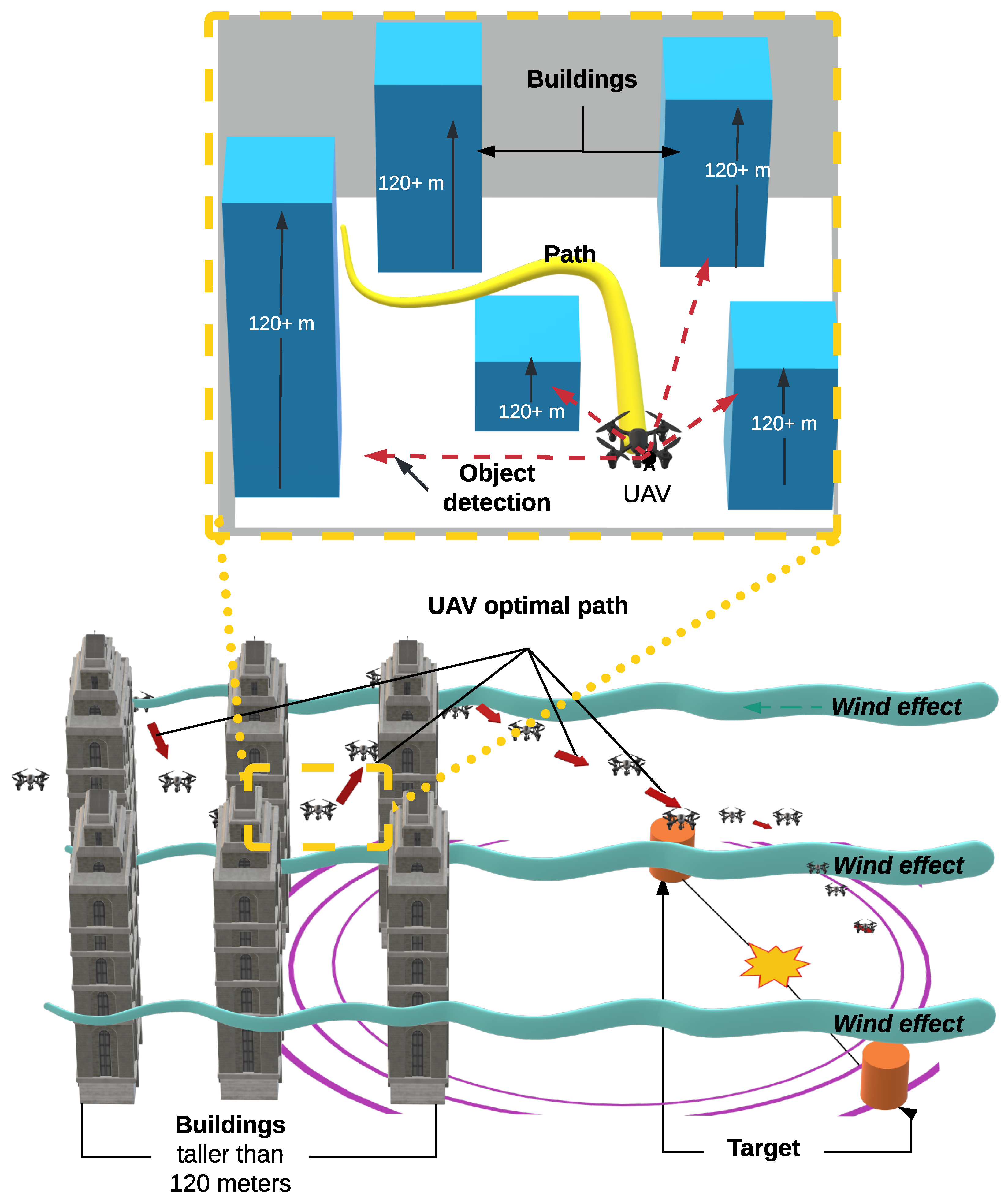
A maximum altitude of 120 m was considered for the UAV’s locomotion toward the target point. This altitude was set according to [63] for urban centers. The UAV can face two situations. The first is when the UAVs fly over regions where the urban buildings are smaller than 120 m. In this case, the heuristic will always have the UAV fly over the smallest buildings to minimize the climatic impact, as shown in Figure 2. For each transition state, the relative distance that the UAV travels is considered. Finally, the UAV may encounter buildings that are higher than the maximum allowable flight altitude. In this case, the UAV cannot fly over the buildings as in the previous situation, so the lateral deviation is the most acceptable alternative. Figure 3 illustrates the behavior of the UAV in the face of obstacles or buildings higher than 120 m.
Algorithm 2 Q-learning for UAV route optimization
Input: Q-table, α [ 0 , 1 ] , γ [ 0 , 1 ] , R, S ( i , j ) , A ( z ) ,
Output: Optimal strategy π * , Optimal router UAV
1:
while e p < = M a x E p i s o d e s  do
2:
    Select an initial state S 0
3:
    while criteria != true or s t e p < = M a x S t e p s  do
4:
        Init a random number  x X [ 0 , 1 ]
5:
        if  x > ϵ  then
6:
           Exploit
7:
            A i = a r g min a A Q ( S , A ) )
8:
           Obtain immediate reward R t Equation (1)
9:
           set the next state S t + 1
10:
           Update Q-table Equation (2)
11:
        else
12:
           Explore
13:
            A i = r a n d [ a 1 , a z ]
14:
           Obtain immediate reward R t Equation (1)
15:
           set the next state S t + 1
16:
           Update Q-table Equation (2)
17:
        end if
ϵ = m i n ϵ + ( m a x ϵ m i n ϵ ) e e p d e c a y R a t e
18:
        end while
19:
    end while
Within the proposed strategy, UAVs act as agents. It has also been considered that each UAV shall receive regular information from weather stations regarding wind conditions in the area of a mission. Based on this, a UAV may be able to calculate an optimized route through Q-learning to reach the desired destination. The algorithm is regularly executed; therefore, the reading of the environment is carried out several times until the UAV reaches the area of interest. The final state of Q-learning processing is the initial point of the next Q-learning processing. Figure 4 illustrates the Q-learning processing while a UAV is traveling.

4.2.1. Agents

In Q-learning aspects, an agent is responsible for exploring an environment and making decisions regarding which actions should be taken during the next t instant based on received rewards. Within the proposed strategy, each UAV acts as an agent. Each agent has an independent Q-matrix; therefore, actions and states that differ within the environment.

4.2.2. States

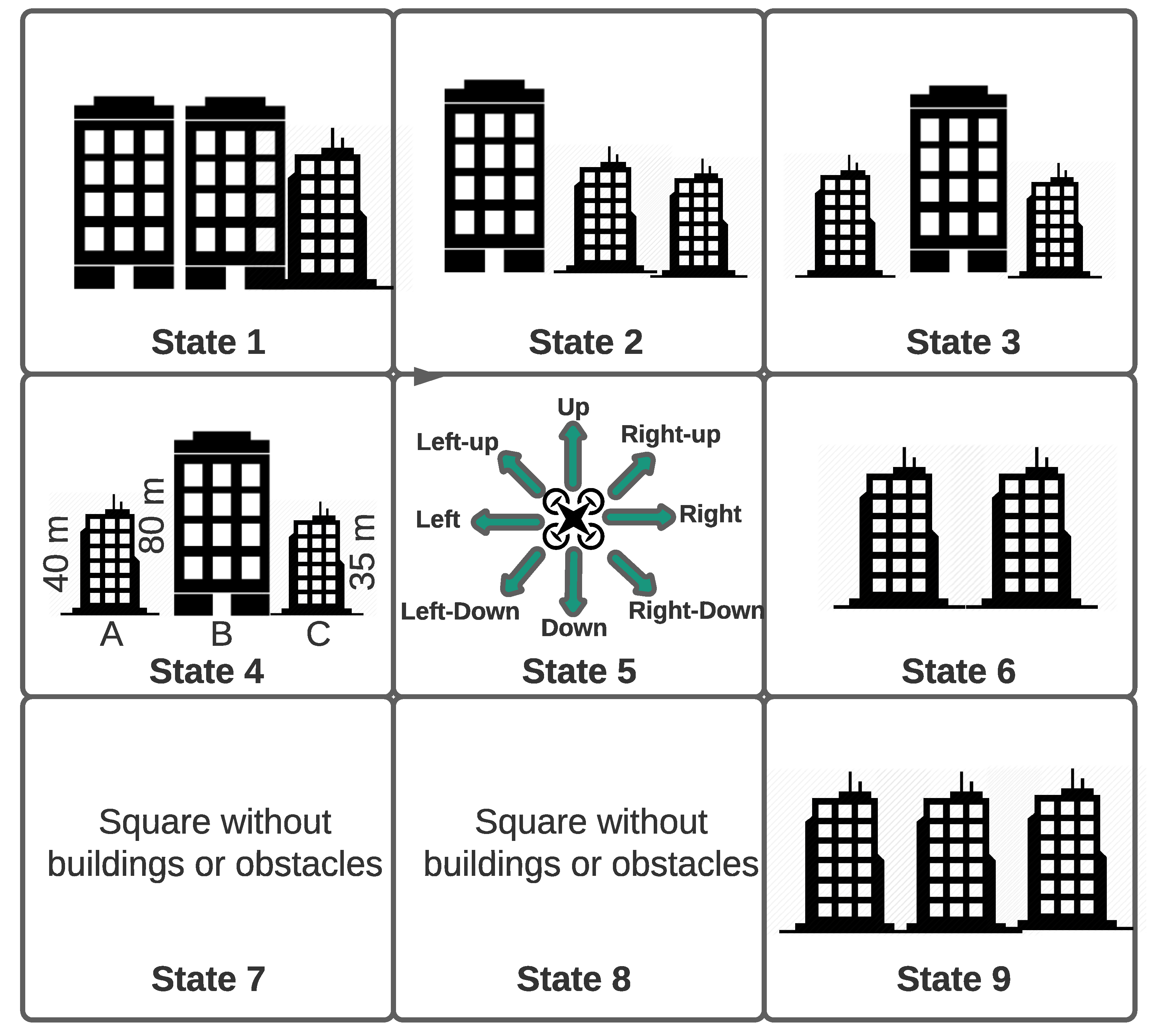
Within the algorithm, the travel space of a UAV is discretized in a grid. Each state represents a potential positioning in the next t instant. Therefore, a UAV should execute actions (traveling) until it reaches an area of interest. Each state is defined by a coordinate that represents a 2D point in the grid. Consequently, for each algorithm episode, a UAV has 9 potential states, as it is illustrated in Figure 5.

4.2.3. Actions

Within the algorithm, each action is defined by a trip. The UAVs may execute an action at each episode towards a new position among 8 potential ones: up, right-up, right, right-down, down, left-down, left, and left-up. A UAV is not allowed to leave a defined grid. In Figure 5, it is possible to observe the potential actions of a UAV.

4.2.4. Reward

In constructing the reward function in this paper, three crucial aspects were considered to achieve the expected optimal result. First, minimize the distance traveled by the UAV to the target point. Second, consider all the obstacle points present in the scenario. And finally, minimizing the impact of the high wind speed. Based on these points, the Equation (8) is considered:
R φ R o b s t a c l e + μ R w i n d + κ R D t a r g e t
where φ , μ , and κ are the weights associated with the obstacles, wind speed, and distance to the point of interest.
According to [64,65,66,67], there is a proportionality relation between the height of a UAV’s flight and the wind velocity; therefore, the higher the altitude of a flight is, the higher the effects encountered by a UAV due to wind velocity shall become. Within this proposal, we have considered that when there are buildings in an area that corresponds to a grid quadrant, a UAV must fly 5 m above the tallest building in the area. To better illustrate this, in Figure 5, the quadrant that was defined by State 4 has buildings with three different heights: 40 m, 80 m, and 35 m. Therefore, a UAV flying under these circumstances should be at an altitude of at least 85 m (5 m above the tallest building in the area). Thus, the reward from this action should correspond to the wind velocity influence at this height. The reward calculation can be observed in Equation (9), where R w i n d is a result of the reward, f V w i n d represents the function of the wind velocity, G represents the environment grid, and B u i l d h e i g h t represents the height, in meters, of the tallest building within that quadrant.
R w i n d V w i n d m a x f V w i n d G i , j ( max B u i l d h e i g h t + 5 )
To measure a reward quantifying the shortest distance traveled by the UAV ( R D t a r g e t ), the following Equation was used (10), where D t a r g e t ( s ) is the distance from the current state to the target, while D t a r g e t ( s 1 ) is the distance from the previous state to the target. Then, in the Equation (11), the reward for detecting obstacles ( R o b s t a c l e ) is calculated, where d i s t o b s t is the distance from the current position of the UAV to each obstacle in the environment and n is the number of obstacles. Both the distance and obstacle detection reward calculations are based on the work of [68].
R D t a r g e t D t a r g e t ( s 1 ) D t a r g e t ( s )
R o b s t a c l e i = 1 n 1 d i s t o b s t i

4.2.5. Q Strategy

In Q-learning, the Q table is defined by all potential states that an agent might encounter. Each value linked to a quadrant within the Q table is directly linked to a reward value. Therefore, the Q table learns with the environment and estimates a value function for each state and action through a series of interactions. The objective of using Q-learning to approach this work is to minimize the effects caused by wind velocity, and to get around obstacles without traveling long distances while the UAVs are traveling to an area of interest. Equation (12) represented maximum Q values using the update rules within the Q table for each iteration. Whence Q ( s t , a t ) represents the current table value for each action, γ is the learning rate, α is the discount factor, and min Q ( s t + 1 , a ) represents the minimum optimal value of a given action on the next phase.
Q ( s t , a t ) Q ( s t , a t ) + α [ R ( s ) + γ max Q ( s t + 1 , a ) Q ( s t , a t ) ]

4.2.6. Algorithm Initialization

UAVs should depart from resource stations. It is important to highlight that each UAV under a scenario is an Agent, and for each Agent, there is a Q matrix. It is considered that the Q matrix of each UAV shall be booted with zeroes. The values of this matrix shall be updated at each iteration following rewards obtained during the exploration of the scenario until the stopping criteria are met.

4.2.7. Stopping Criteria

Two stopping criteria have been utilized within the proposed solution. The first criteria are whence a UAV reaches an area of interest, referred to as a maximum reward. It has been considered that this area corresponds to the location in which an optic fiber has been burst. Should the algorithm not reach these criteria, the algorithm shall stop when a UAV has moved throughout a maximum number of MaxSteps iterations within the grid.

4.3. Evaluation Metrics

To evaluate the behavior of the solution using reinforced learning techniques, some metrics must be considered, such as the distance traveled by the UAV, the energy consumption, the effects of wind speed, and finally the success rate in reaching the target point without colliding or losing the route.

4.3.1. Distance Traveled

This metric is used to determine which reinforcement learning technique managed to reach the point of interest with the shortest possible distance, despite the presence of obstacles and adverse weather conditions. To calculate this metric, we need to consider the absolute distance, i.e., the Euclidean distance between the current state s and the next state s + 1 Equation (13). Then, it is necessary to check whether the flight altitude has changed between state s and state s + 1 to determine a new distance ( D r e l a t i v e ) traveled by the UAV (Equation (14)). Finally, the total distance traveled by each UAV is stored (Equation (15)) where K is the number of UAVs, t is the time needed for the route, and P L is the matrix with the distance covered by each UAV to the respective target point.
D a b s o l u t e ( x ( s ) x ( s + 1 ) ) 2 + ( y ( s ) + y ( s + 1 ) ) 2
D r e l a t i v e = H ( s ) H ( s + 1 ) ( D a b s o l u t e ) 2 + ( H s H ( s + 1 ) ) 2 o t h e r w i s e D a b s o l u t e
P L i , j i = 1 k j = 1 p D r e l a t i v e ( i , j )
where K is the number of UAVS, t is the time instants spent on the route, and P L is the matrix with the distance traveled from each UAV to the respective point of interest.

4.3.2. Energy Consumer

The power consumption E c o n s u m e r is an important factor that determines the deployment time of the UAV. In this work, two types of situations are considered in which power consumption plays a role. First, when the UAV is moving to the target point, i.e., when it is under the direct influence of the wind (Equations (17) and (18)). At the second moment, when the UAV establishes communication, i.e., hovers in the air without being influenced by the wind (Equation (16)). Gravity g, wind speed v w i n d , payload m, and distance traveled D have a direct impact on the drone’s power consumption during missions [28,69,70].
E c o n s u m e r m g t o p e r a t i o n
v p v U A V + v w i n d
E c o n s u m e r ( m v p 2 D ) + ( m g D ) 2 v U A V
where v p is the propulsion speed required for UAV flight, t o p e r a t i o n is the time the UAV performs its service in hover, and v U A V is the displacement speed of the UAV.
Through the work [28] it was possible to infer the wind effects according to Equation (18) have been illustrated in Figure 6, in which the higher the wind velocity is, the power consumption increases exponentially, while the distance influences a rectilinear behavior.

4.3.3. Success Rate

This metric is intended to determine how many times the UAV successfully reached the target N s u c c e s s within a series of N attempts. The value of this metric is calculated by Equation (19).
S R N s u c c e s s N

4.3.4. Wind Speed

To calculate the average wind speed at different altitudes, one must know a reference value at the same location at a certain altitude. Here z 0 is the value of the roughness factor that depends on the terrain of interest, as shown in Table 1. h 1 is the altitude at which you know the wind speed v 1 , which you can get from the metrology department of the region. The h 2 is the altitude at which you want to calculate the speed. Using what is discussed in [71], the logarithmic profile of wind speed v 2 can be measured according to the Equation (21):
v 2 = v 1 l n h 2 z 0 l n h 1 z 0
v p a t h ( i , j ) = i = 1 k j = 1 t v 2 ( i , j )
where K is the number of UAVs and v p a t h is the wind speed observable by each UAV at each instant t.

5. Experiments and Tests

To ensure the reliability of the strategy proposed in this work, it was decided to perform some tests illustrating the behavior of the chosen reinforcement learning techniques in the face of some scenarios with different speeds and a variable number of obstacles. The experiments were divided into 5 sections, summarized in Table 2 and described in detail in the next subsections. For the development of this work, the Python programming language was used to build the algorithms discussed in this work and the MATLAB (student version) was used to plot the figures.
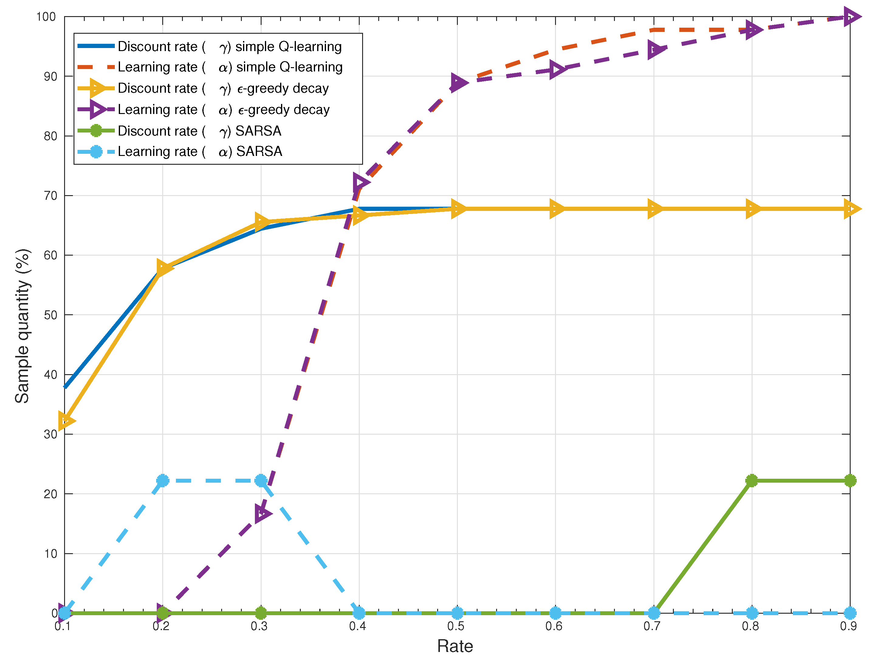
To select the parameters of the heuristics based on reinforcement learning, such as the learning rate ( α ) and the discount rate ( γ ), numerous tests were performed with 1000 different scenarios in which wind speed and obstacles were randomly inserted into the environment with dimensions of 30 × 30 cell grids. The tests were designed to show the extent to which the variation of α and γ is fundamental for the UAV to reach the target point without deviating from the route or colliding with obstacles. After this, the success rate of the UAV to reach the desired goal in each scenario within the sample is calculated. The values α and γ are varied between 0.1 and 0.9, and after completing the tests, was found that for 100 % of the samples, Simple Q-learning and Q-learning with ϵ -greedy decay had a value of α equal to 0.9, while for SARSA the same value of learning rate covered 23 % of the samples. For ( γ ), SARSA obtained the best results for rates of 0.2–0.3, while the other techniques obtained better results for rates above 0.5. Figure 7 illustrates the results obtained in this evaluation.
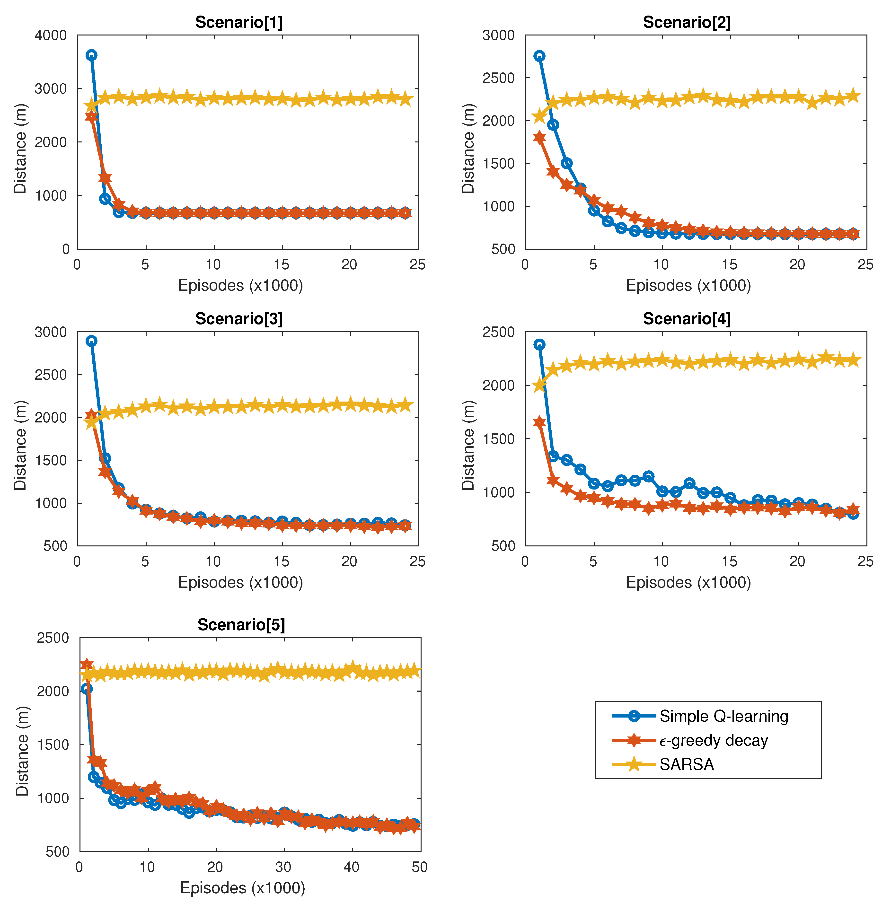
After analyzing the learning rate and discount factor variables, the project team needed to know the number of episodes required to train the Q table. For each experiment, the convergence curve was analyzed in terms of minimizing the distance traveled by the UAV as a function of the iterated episodes, according to [68]. From Figure 8, it can be seen that the convergence process of the algorithms tends to require more iterations as the number of obstacles and points with high wind speed increases, which directly affects the algorithm processing time. In Experiment 1 with only one obstacle, the convergence of Q-learning with ϵ -greedy decay and Simple Q-learning is estimated to be 2500 and 3100 episodes, respectively, while in Experiment 5 with multiple obstacles and multiple points of high wind speed, approximate convergence is reached at 41,000 and 43,000 episodes, respectively. Despite the high value of convergence, the algorithm is executed in a few seconds, varying from the lowest to the highest complexity between 5.67 s and 37.43 s. In all, the 1000 simulations took in average 4 h:48 mim:56 s for SARSA, 5 h:28 mim:26 s for Simple Q-learning, 6 h:15 mim:13 s for egreedy decay Q-learning. In most experiments, Q-learning converged with ϵ -greedy decay faster than the other heuristics and proved to be the most efficient of the techniques. In all experiments, SARSA proved to be quite inefficient during the convergence process and almost always increased the distance traveled by the drone because the heuristic directs the UAV to redundant routes, i.e., often gets stuck at isolated points on the grid and persistently repeats the same steps during iterations.
For the values of γ and α we use the values obtained from Figure 7 while φ , μ and κ are respectively 0.65, 0.75 and 0.95.

5.1. Experiment 1

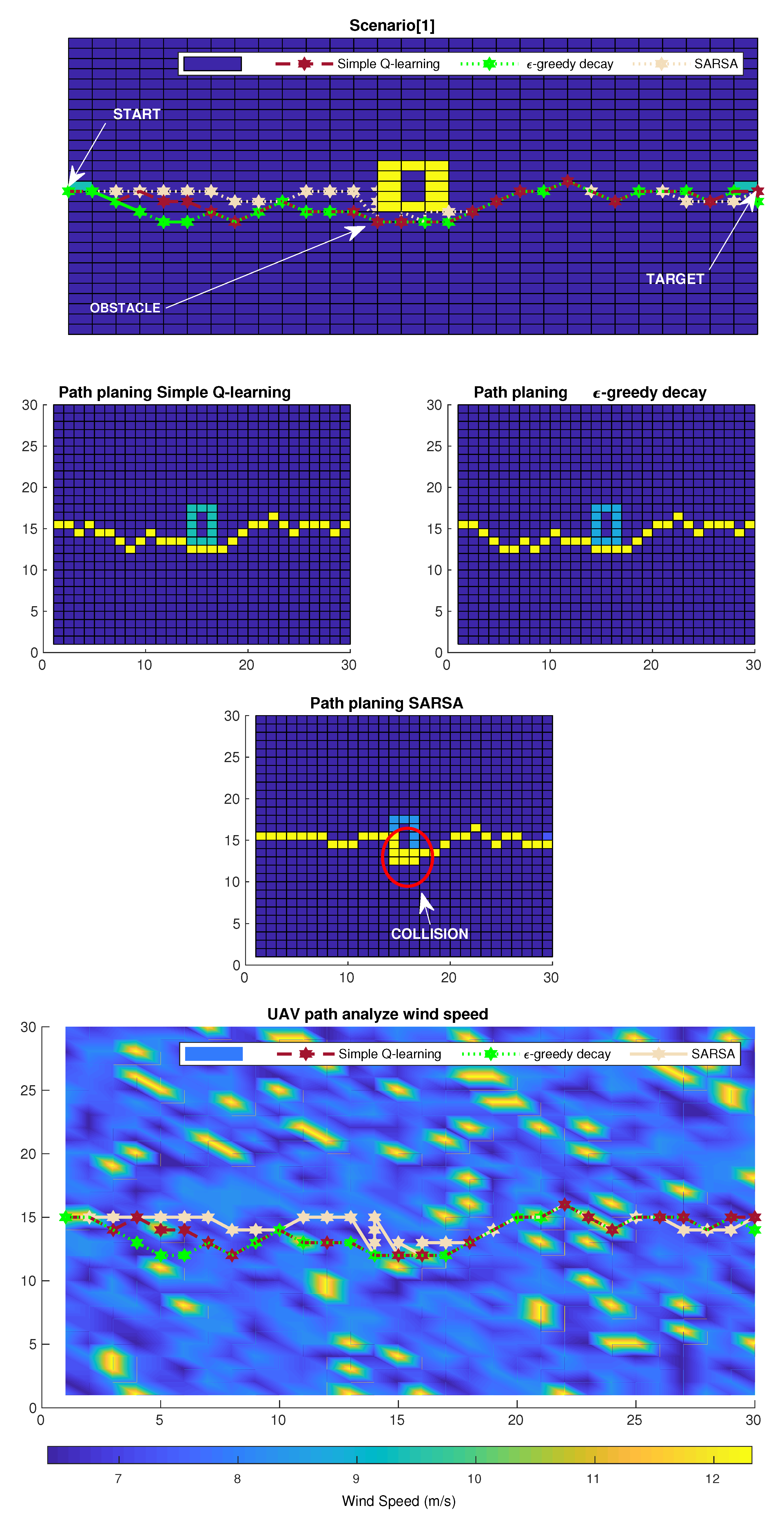
Experiment 1 was designed to represent the case with less complex obstacles, considering only 1. Both Q-learning and ϵ -greedy decay and Simple Q-learning followed similar routes, always favoring the shortest path. Unlike the other techniques, SARSA collided with the obstacle and remained stuck in the condition where it followed a repetitive path. For the wind speed points, the Q-learning heuristic with ϵ -greedy decay had an advantage in the first moments because it avoided a point with high wind speed. Figure 9 illustrates the behavior of the heuristics for Experiment 1.

5.2. Experiment 2

Experiment 2 is configured with 2 heterogeneous obstacles in the center and with randomly placed wind speed points. Q-learning with ϵ -greedy decay tracked a route more toward the low wind speed zones compared to Simple Q-learning. Figure 10 illustrates the behavior of the heuristics for Experiment 2.

5.3. Experiment 3

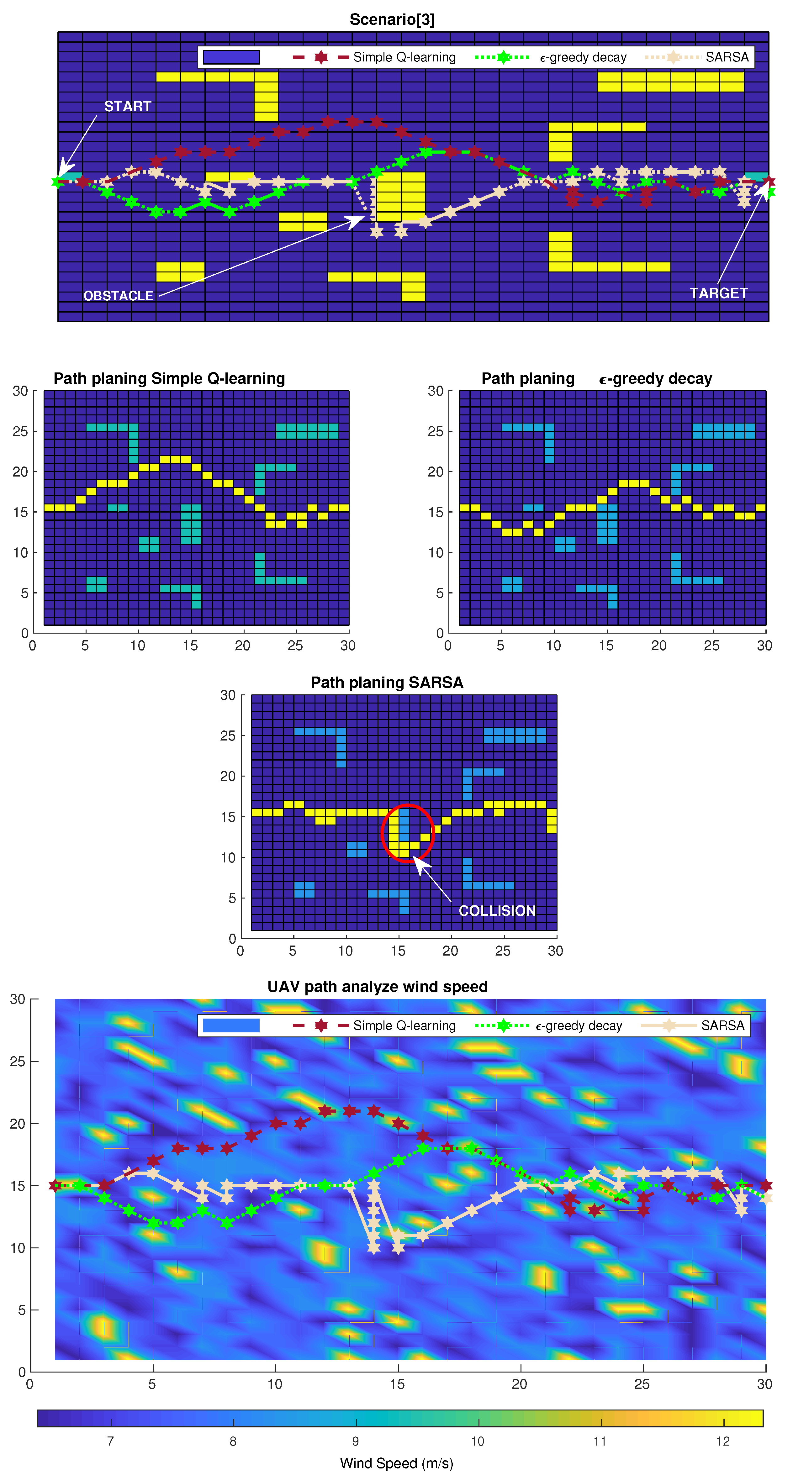
In Experiment 3, the scenario is configured with 9 heterogeneous obstacles distributed throughout the network. The wind speed was randomized as in the other experiments. In the first half of the path, Simple Q-learning takes a similar path to the Q-learning with ϵ -greedy decay in Experiment 2, but gets into more high-speed points, while the Q-learning based one ϵ -greedy decay follows a path with fewer turns and low gusts. Figure 11 illustrates the behavior of the heuristics for Experiment 3.

5.4. Experiment 4

Experiment 4 elaborated the worst-case scenario for UAV flight, adding a grid with 49 obstacles in the center of the grid and positioning points of high wind speed between the obstacles. In this situation, both the heuristic based on ϵ -greedy decay and Simple Q-learning ignored the wind gusts and prioritized the obstacles and the distance to the target. SARSA Figure 12 illustrates the behavior of the heuristics for Experiment 4.

5.5. Experiment 5

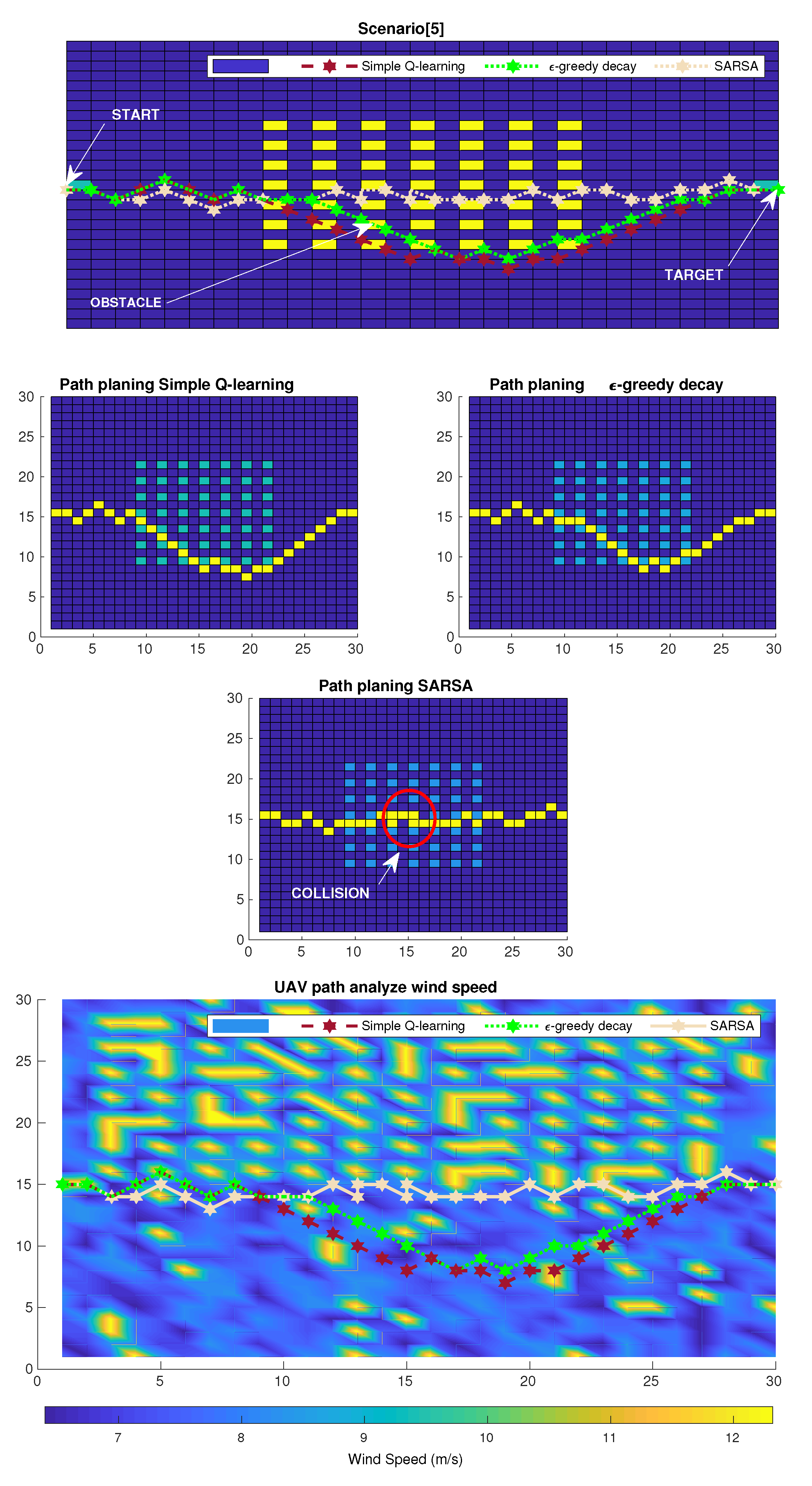
In this experiment, the scenario was configured similarly to Experiment 4 but differed in the placement of high wind speed points plotted in the upper half of the grid. Despite the generated SARSA route that assigned a collision to the UAV, all techniques avoided the zone of high wind influence, especially Q-learning with ϵ -greedy decay, which created a shorter route through fewer gust points than the route determined with Simple Q-learning. Figure 13 illustrates the behavior of the heuristics for Experiment 5.

6. Simulation Results

6.1. Simulation Scenario

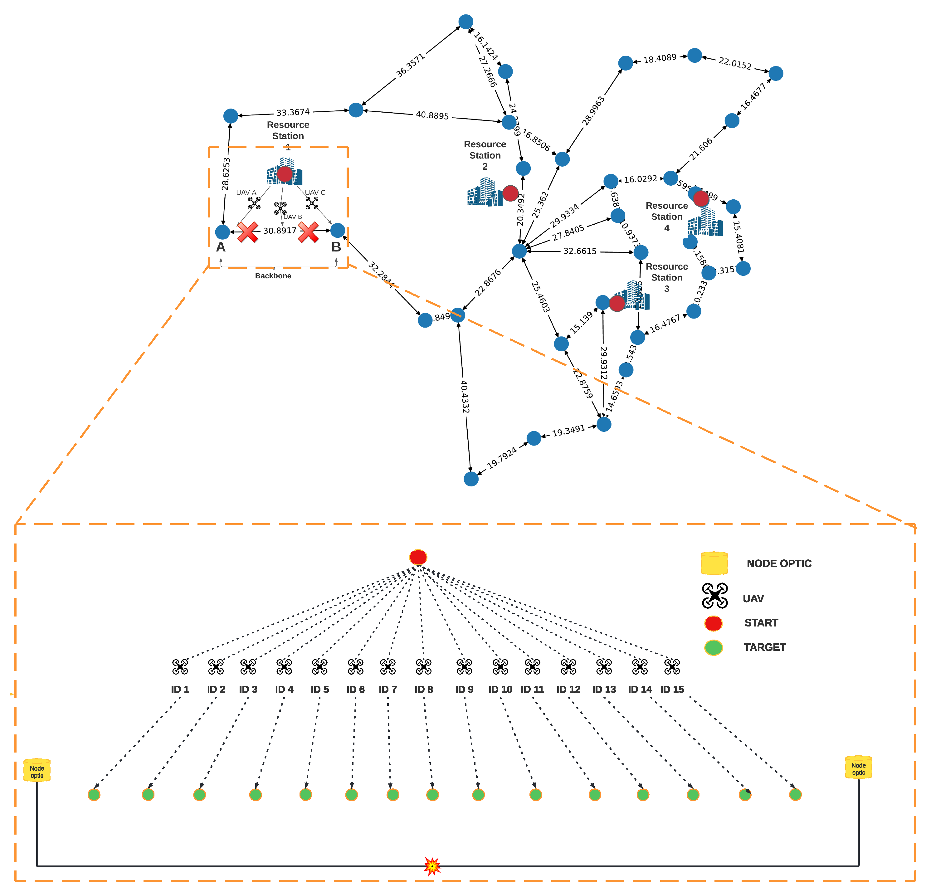
For our simulations, was considered the topology described in [72] and shown in Figure 14. We considered the cost and installation of a UAV-based air telecommunication structure in terms of the number of UAVs and communication interfaces radio. Among several disaster scenarios, the case with the highest number of broken connections within the Stockholm topology in Sweden was selected.
The existence of four points has been considered, named resource stations, from which the UAVs should depart. Upon the actuation of an emergency, therefore, an optic fiber cutoff, a UAV departs from the nearest station to the mission location, which in this case, is Resource Station 1. Subsequently, the heuristics-based reinforcement learning is responsible for coordinating the UAVs to deviate from the adversities within the area such as windy zones and physical obstacles.
To characterize the mission, an optic fiber link was chosen among all of those within the topology, which should be inactive or malfunctioning. The selected enlace has 30.89 km of extension between two backbones (A & B), (Figure 14) in which 15 UAVs have been distributed equidistantly 2 km from one another according to the communication enlace specs based on free-space optics (FSO) [73]. Table 3 breaks down all parameters adopted for this experiment.

6.2. Numerical Results

To prove the potential of this work as an alternative for route optimization of UAVs in urban scenarios, was considered the distance traveled, wind speed, power consumption, and success rate as performance indicators between techniques based on reinforcement learning: SARSA, Simple Q-learning and ϵ -greedy decay. In addition, we compared our method that takes climatic conditions into account with the methods based only on obstacles, which again are widely discussed in the literature. The group also considers, in the comparison, a naive strategy where the UAVs fly in a straight.
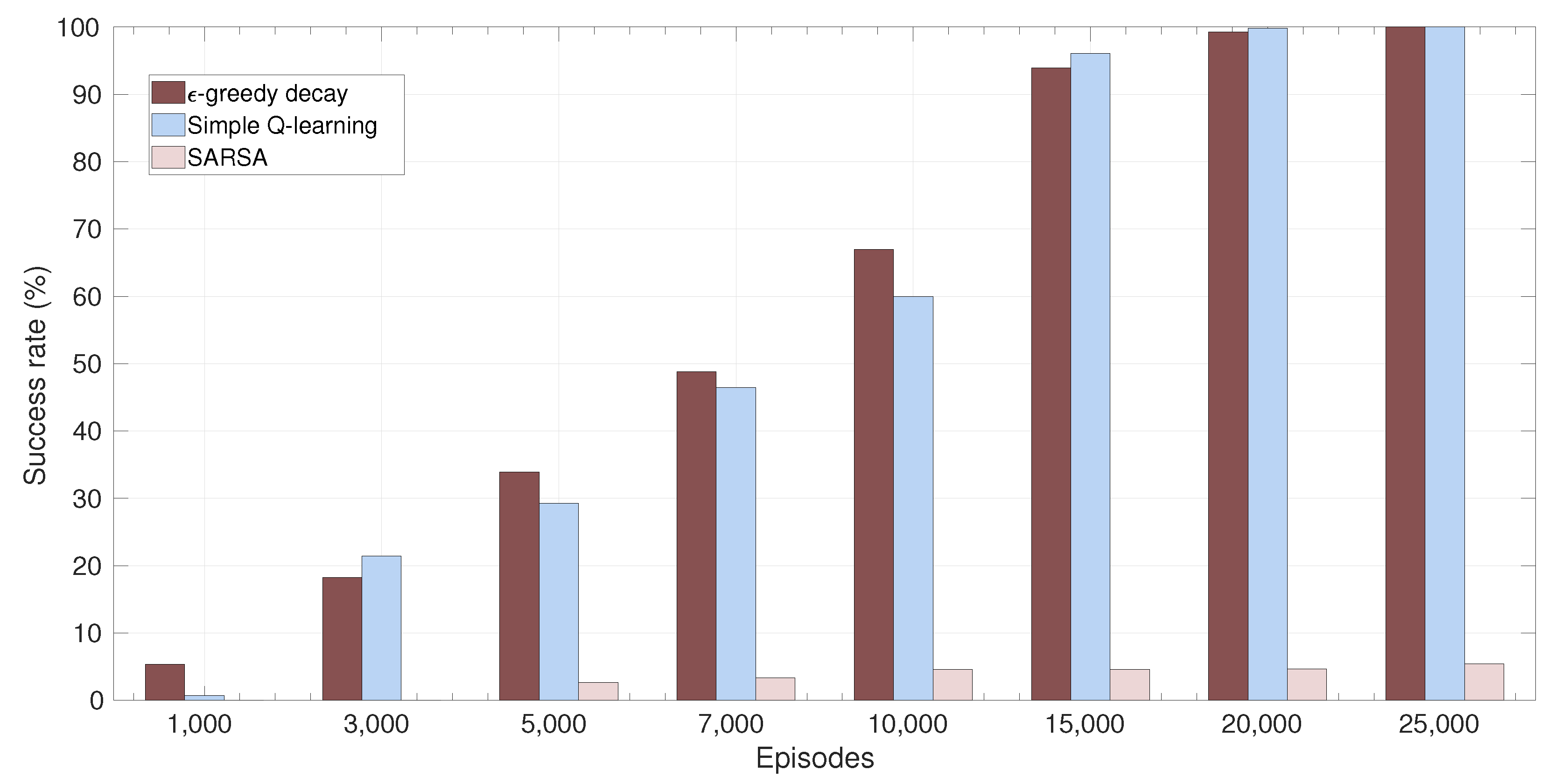
To determine the probability of success of the UAV in reaching the final destination, we checked the success rate for each processing of the algorithm along the route and then averaged these values as a function of each specified episode boundary. An 8-element set represented by the number of episodes is used for the SARSA, Simple Q-learning, and ϵ -greedy decay (1000, 3000, 5000, 7000, 1000, 15,000, 20,000, 25,000). As shown in Figure 15, the success rate of heuristics based on Simple Q-learning and ϵ -greedy decay increased with an increasing number of episodes, in contrast to SARSA, which evolved little and achieved an average increase in the success rate of 0.77% with an increasing number of episodes, while ϵ -greedy decay had a rate of 13.52%, followed by Simple Q-learning with 14.18%. Despite the wider variation of Simple Q-learning, it is important to note that ϵ -greedy decay for elements 1000 to 10,000 had the highest success rates during the mission among all the techniques discussed. This can be an alternative if you want to make faster decisions at the expense of the optimal path, i.e., if you want to switch between an automated alternative and another manual or less intelligent alternative, such as steering the UAV over all obstacles in a straight line.
Was added to SARSA, Simple Q-learning, and ϵ -greedy decay strategies that involve minimizing the effects of wind speed, avoiding obstacles, and minimizing distance. For heuristics whose strategy is only about obstacle avoidance, the simple Q-learning adapted for this purpose was used. The naive solution is the strategy where a UAV travels in a straight line at the lowest possible altitude without colliding with obstacles. For this purpose, was consider the processing grid of algorithms configured as 30 × 30, where each state can be a possible displacement of the UAV. 25,000 episodes were fixed for all techniques. We determined γ and α according to the results from Figure 7, i.e., a learning rate of 0.9 and a discount factor of 0.5 for Simple Q-learning and e p s i l o n -greedy decay, while for SARSA the learning rate was 0.3 and the discount factor was 0.8. The same values were used for φ , μ , and κ for all techniques based on reinforcement learning, except for the heuristic that aims to avoid obstacles in its composition, we use 0 to determine the value m u . Table 3 shows all parameters used during the simulations.
In Figure 16 we can measure the wind variations experienced by each UAV along the path considering the different algorithms. In this Figure, we can see that the heuristics that incorporate the wind speed minimization strategy stand out compared to the naive solution. However, for UAVS 5, 9, 12, 14, and 15, SARSA had a worse result than the solution that only considers the obstacles, this happens because when a heuristic is not able to succeed in elaborating the route, either due to collision or discontinuity of the path to the target, it is automatically replaced by the route of the naive solution from the interrupted point. Therefore, the complexity of the path taken by UAVs 5, 9, 12, 14, and 15 SARSA has approached the naive solution, which makes this strategy less attentive to changes in the scenario compared to others that identify high-speed zones from the wind, making it a less efficient solution than Simple Q-learning and ϵ -greedy decays. The proposed strategy not only reduces the effects of wind speed but was also able to minimize the distance traveled by the UAV. This is due to the minimized relative distance, as the heuristic used in this work aims to keep the UAV flight at lower altitudes where the wind speed is lower to ensure lower peak fluctuations, which significantly reduce the relative distance traveled by the UAV.
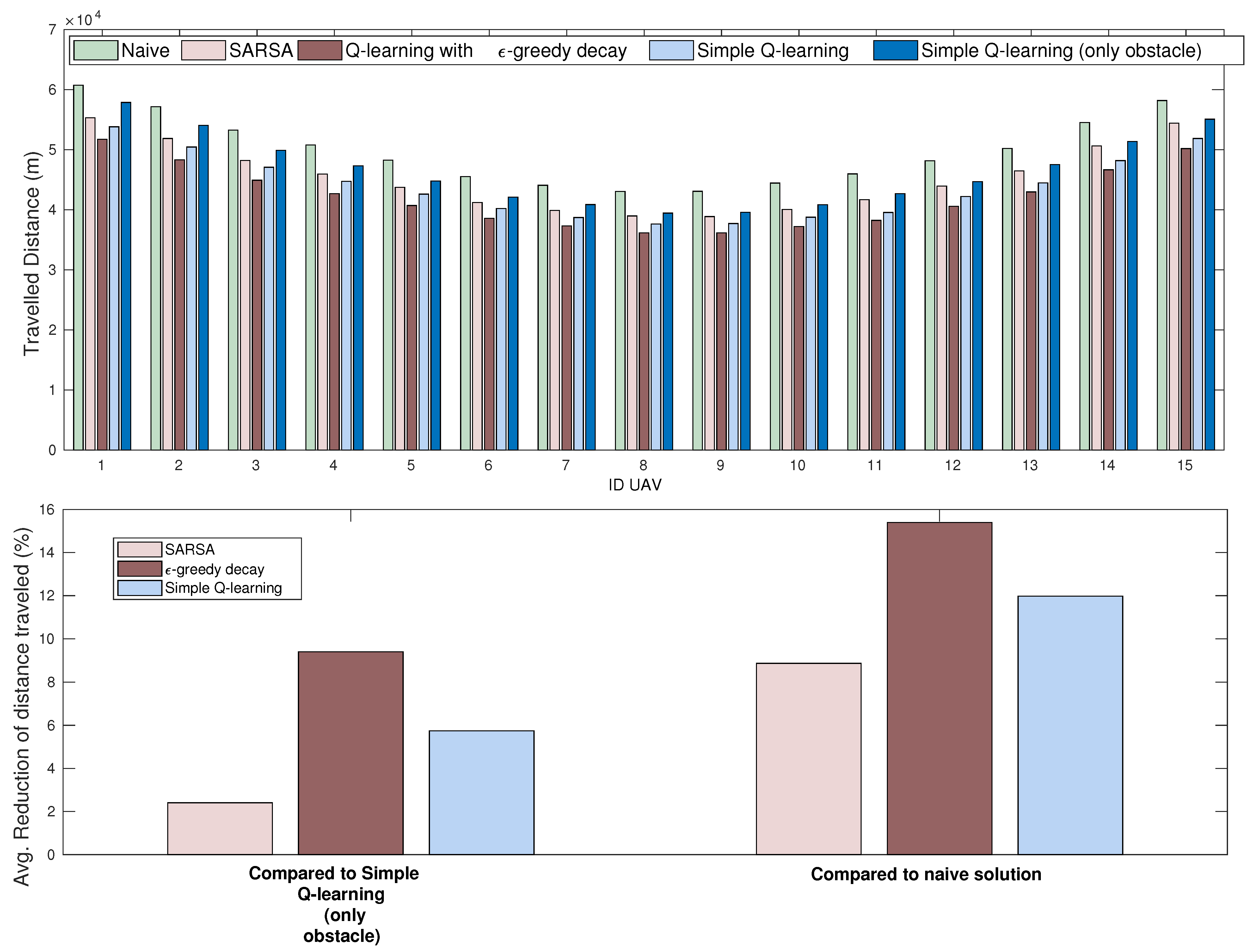
The results shown in Figure 17 refer to the distance traveled by each UAV during the mission. Here we can see that both Simple Q-learning and ϵ -greedy decays reduced the trajectory for all UAVS compared to the other approaches. On average, Simple Q-learning reduced trajectories from 5.83% to 11.94% compared to Simple Q-learning (obstacles only) and Naive, respectively, while ϵ -greedy decays performed slightly better with an estimated 9.39% compared to Simple Q-learning (obstacles only) and achieved a reduction of 15.39% for Naive. As we know from the topology illustrated in Figure 14, the UAVs do not travel the same distances. For example, the UAV with ID 8 travels a shorter distance than the UAV with ID 15 because they occupy different points in the UAV network. To find out how much distance affects the performance of the solutions, we took the value of the distance of the strategy that achieved the best ( ϵ -greedy decays) and worst (Naive) results for each UAV at the ends (1, 2, and 15) and in the center (7, 8, and 9), and shortly calculated the average between the edge and center points to obtain a value for the path reduction between the closer and farther UAVs of the target. we obtained a distance reduction of approximately 15.82% for the central UAVs, while for the edge UAVs the reduction was 14.26%, i.e., a gain of 1.56% relative to the edge UAVs. Based on these results, we can see the tendency that points of interest closer to the starting points have better distance reduction results.
The energy consumed by the UAV during flight is the result of the varying effects of wind speed, load, and distance traveled [28,69,70]. From Figure 18, it is clear that the solutions that considered wind speed as a strategy obtained the lowest results in energy consumption during the UAV flight, with a maximum reduction of 15.93% decreases by the ϵ -greedy based heuristic in contrast to the naive case, however, our group must pay attention to the behavior of the results, which in turn is strongly influenced by the distances traveled by each UAV, proving that although wind speed is a relevant factor in the energy consumption formula, the distance traveled is still the main factor limiting the autonomy of the UAVs during the missions. In this sense, the results have shown that the intelligent heuristic proposed in this work not only finds routes with lower wind influence but also significantly minimizes the distances traveled by the UAVs.
Energy optimization is fundamental to extending the lifetime of UAVs during missions. Based on the results of this work, we were able to: diversify the scenarios (different numbers of obstacles and high wind speed points randomly selected and concentrated in different parts of the network); analyze the behavior of reinforcement learning techniques, such as the definition of the best parameters. Finally, the scenario was chosen based on the optical topology of Stockholm, Sweden, and then applied what was discussed in the experiments, where it was possible to analyze graphically the behavior of UAVs in flight.
Finally, our analyses not only reduced the distances traveled by UAVs but also minimized the impact of high wind speeds. This is because high wind gusts not only contribute negatively to energy efficiency but can also cause damage and disruption to the UAV’s navigation, leading to loss of control and consequently financial and safety losses as the UAV is exposed to destruction or even causes serious accidents in urban environments.

6.3. Results and Discussion

In the currently implemented model, the wind velocity vector is always opposite to the UAVS velocity vector. This assumption is somewhat restrictive because, in certain situations, the energy consumption depends on how the angle between the vectors is arranged. During the scenario characterization, the buildings were randomly arranged in the scenario, i.e., not faithfully characterizing the urban infrastructure of Stockholm (Sweden), Nevertheless, the results obtained showed that the energy consumption of the UAVS can be reduced by using reinforcement learning. Finally, the project team did not produce a model that would provide an optimal solution to the problem addressed. Moreover, our group is aware that it is interesting to study how far the locally optimal solutions obtained by the proposed method are from the globally optimal solutions, which does not harm the analysis of the results obtained, since the main objective of the paper was fulfilled. Our model is fully flexible and suitable to include, in future works, new analyses to mitigate the current limitations and make it more efficient and robust.
For future work, our team aims to investigate other machine learning techniques such as deep Q-learning and neuro-fuzzy, and compare them with what has already been implemented in this study. We also intend to consider the energy consumption during the communication between the UAVs during the provision of the wireless communication service or bridge. In addition, we plan to incorporate a control unit into the UAV in a controlled environment, enabling the management of its flight through the reinforcement learning techniques discussed in this study. This will allow us to consider both heterogeneous obstacles and the variation of wind speed experienced by the UAV. We will compare the results of the test bed with those obtained in simulations.

7. Conclusions

In this work, a new method has been proposed to contribute to the path optimization of UAVS in urban scenarios. The proposed strategy aims to minimize the distance traveled and reduce the effects of wind speed that UAVs are exposed to minimize energy consumption. The heuristic was implemented using three reinforced learning methods (Simple Q-learning, ϵ -greedy, and SARSA) and compared to a naive solution and a path optimization method in multi-obstacle scenarios, a solution widely studied in the literature.
Our group have performed several tests to find out the values of the variables that best fit the problem studied in this paper, and we have found the values of γ , α , and the number of episodes that best fit our solution. Several experiments were conducted to prove the efficiency of our method given the variability of the scenarios (obstacles and high wind speed points), and in most experiments, our solution avoided both obstacles and high wind speed areas.
To prove the efficiency of the proposed method, the project team conducted a case study considering the topology of the metropolitan optical network in Stockholm, Sweden. The numerical results of the simulations showed that the solution based on climatic factors could reduce the power consumption of the flying network from 2 % to 15.93 % compared to naive heuristics and those considering only physical obstacles, which can help to extend the deployment time of UAVs.
The strategy proposed in this work was tested by simulating an urban scenario consisting of buildings of different heights, similar to real urban environments. In this case, the UAV chose the best route based on the shortest distance traveled and the lowest wind speed. The results were obtained using the different reinforced learning methods tested in this work. The method that stood out the most among all the scenarios tested was Q-learning with ϵ -greedy. This is because it was able to find the shortest distances and the regions with the lowest wind speed. On the other hand, the SARSA method was generally not more efficient than the other two Q-learning-based methods for any of the performance metrics considered. Finally, the results of this work contribute to the increasing efficiency of UAV routing, which in turn contributes to the increasing use of UAVs in civil applications, as expected for smart cities.

Author Contributions

Conceptualization, A.S., R.A., E.C., J.A. and C.F.; methodology, A.S. and R.A.; validation, A.S.; formal analysis J.A. and C.F.; investigation A.S.; writing—original draft preparation, A.S., E.C. and J.A.; writing—review and editing, A.S., E.C., and J.A. All authors have read and agreed to the published version of the manuscript.

Funding

This research received no external funding.

Institutional Review Board Statement

Not applicable.

Informed Consent Statement

Not applicable.

Data Availability Statement

Not applicable.

Acknowledgments

The authors would like to thank the CAPES—Coordination for the Improvement of Higher Education-Finance Code 001 and PROPESP/UFPA.

Conflicts of Interest

The author declares no conflict of interest.

Abbreviations

The following abbreviations are used in this manuscript:
UAVUnmanned aerial vehicles
CITInformation and communication technology
BANsBody area networks
LoSLine of sight
NTSBThe National Transportation Safety Board
SARSA(State − action − reward − state − action)
MDPMarkov Decision Process
VTOLVertical Take-Off and Landing
FSOFree-space optics
Q-LQ-learning
φ Obstacle weights
μ Wind speed weights
κ Distance weights
R o b s t a c l e Obstacle reward
R w i n d Wind speed reward
R D t a r g e t Distance of target reward
R o b s t a c l e Obstacle reward
V w i n d m a x Maximum wind speed
D a b s o l u t e Absolute distance
KMumber of UAVS
v p Propulsion speed
DDistance travaled
mPayload
D r e l a t i v e Relative distance
B u i l d h e i g h t Height of the building
z 0 Roughness factor
h 2 Altitude to calculate the speed
h 1 Initial altitude the speed
v U A V UAV speed
v w i n d Wind speed
γ Discount rate
α Learning rate

References

  1. Dagooc, E.M. IBM urged LGUs to embrace the’Smarter city’initiative. Philipp. Star. Retrieved March 2010, 3, 2011. [Google Scholar]
  2. Mosannenzadeh, F.; Vettorato, D. Defining smart city. A conceptual framework based on keyword analysis. TeMA-J. Land Use Mobil. Environ. 2014, 16, 684–694. [Google Scholar] [CrossRef]
  3. Sánchez-Corcuera, R.; Nuñez-Marcos, A.; Sesma-Solance, J.; Bilbao-Jayo, A.; Mulero, R.; Zulaika, U.; Azkune, G.; Almeida, A. Smart cities survey: Technologies, application domains and challenges for the cities of the future. Int. J. Distrib. Sens. Netw. 2019, 15, 1550147719853984. [Google Scholar] [CrossRef]
  4. Visvizi, A.; Lytras, M.D.; Damiani, E.; Mathkour, H. Policy making for smart cities: Innovation and social inclusive economic growth for sustainability. J. Sci. Technol. Policy Manag. 2018, 9, 126–133. [Google Scholar] [CrossRef]
  5. Silva, B.N.; Khan, M.; Han, K. Towards sustainable smart cities: A review of trends, architectures, components, and open challenges in smart cities. Sustain. Cities Soc. 2018, 38, 697–713. [Google Scholar] [CrossRef]
  6. Medina-Borja, A. Editorial column—Smart things as service providers: A call for convergence of disciplines to build a research agenda for the service systems of the future. Serv. Sci. 2015, 7, 2–5. [Google Scholar] [CrossRef]
  7. Gupta, L.; Jain, R.; Vaszkun, G. Survey of important issues in UAV communication networks. IEEE Commun. Surv. Tutorials 2015, 18, 1123–1152. [Google Scholar] [CrossRef]
  8. Mehta, P.; Gupta, R.; Tanwar, S. Blockchain envisioned UAV networks: Challenges, solutions, and comparisons. Comput. Commun. 2020, 151, 518–538. [Google Scholar] [CrossRef]
  9. Maddikunta, P.K.R.; Hakak, S.; Alazab, M.; Bhattacharya, S.; Gadekallu, T.R.; Khan, W.Z.; Pham, Q.V. Unmanned aerial vehicles in smart agriculture: Applications, requirements, and challenges. IEEE Sensors J. 2021, 21, 17608–17619. [Google Scholar] [CrossRef]
  10. De Alwis, C.; Kalla, A.; Pham, Q.V.; Kumar, P.; Dev, K.; Hwang, W.J.; Liyanage, M. Survey on 6G frontiers: Trends, applications, requirements, technologies and future research. IEEE Open J. Commun. Soc. 2021, 2, 836–886. [Google Scholar] [CrossRef]
  11. Tisdale, J.; Kim, Z.; Hedrick, J.K. Autonomous UAV path planning and estimation. IEEE Robot. Autom. Mag. 2009, 16, 35–42. [Google Scholar] [CrossRef]
  12. Grasso, C.; Schembra, G. Design of a UAV-based videosurveillance system with tactile internet constraints in a 5G ecosystem. In Proceedings of the 2018 4th IEEE Conference on Network Softwarization and Workshops (NetSoft), Montreal, QC, Canada, 25–29 June 2018; pp. 449–455. [Google Scholar]
  13. Ullah, S.; Kim, K.I.; Kim, K.H.; Imran, M.; Khan, P.; Tovar, E.; Ali, F. UAV-enabled healthcare architecture: Issues and challenges. Future Gener. Comput. Syst. 2019, 97, 425–432. [Google Scholar] [CrossRef]
  14. Tang, C.; Zhu, C.; Wei, X.; Rodrigues, J.J.; Guizani, M.; Jia, W. UAV placement optimization for Internet of Medical Things. In Proceedings of the 2020 International Wireless Communications and Mobile Computing (IWCMC), Limassol, Cyprus, 15–19 June 2020; pp. 752–757. [Google Scholar]
  15. Mozaffari, M.; Kasgari, A.T.Z.; Saad, W.; Bennis, M.; Debbah, M. Beyond 5G with UAVs: Foundations of a 3D wireless cellular network. IEEE Trans. Wirel. Commun. 2018, 18, 357–372. [Google Scholar] [CrossRef]
  16. Li, B.; Fei, Z.; Zhang, Y. UAV communications for 5G and beyond: Recent advances and future trends. IEEE Internet Things J. 2018, 6, 2241–2263. [Google Scholar] [CrossRef]
  17. Pham, Q.V.; Zeng, M.; Ruby, R.; Huynh-The, T.; Hwang, W.J. UAV Communications for Sustainable Federated Learning. IEEE Trans. Veh. Technol. 2021, 70, 3944–3948. [Google Scholar] [CrossRef]
  18. Zeng, Y.; Zhang, R.; Lim, T.J. Wireless communications with unmanned aerial vehicles: Opportunities and challenges. IEEE Commun. Mag. 2016, 54, 36–42. [Google Scholar] [CrossRef]
  19. Şahin, H.; Kose, O.; Oktay, T. Simultaneous autonomous system and powerplant design for morphing quadrotors. Aircr. Eng. Aerosp. Technol. 2022, 94, 1228–1241. [Google Scholar] [CrossRef]
  20. Zeng, Y.; Zhang, R. Energy-efficient UAV communication with trajectory optimization. IEEE Trans. Wirel. Commun. 2017, 16, 3747–3760. [Google Scholar] [CrossRef]
  21. Wu, F.; Yang, D.; Xiao, L.; Cuthbert, L. Energy consumption and completion time tradeoff in rotary-wing UAV enabled WPCN. IEEE Access 2019, 7, 79617–79635. [Google Scholar] [CrossRef]
  22. PAHL, J. Flight recorders in accident and incident investigation. In Proceedings of the 1st Annual Meeting, Washington, DC, USA, 29 June–2 July 1964; p. 351. [Google Scholar]
  23. Lester, A. Global air transport accident statistics. In Proceedings of the Aviation Safety Meeting, Toronto, ON, Canada, 31 October–1 November 1966; p. 805. [Google Scholar]
  24. Li, W.; Wang, L.; Fei, A. Minimizing packet expiration loss with path planning in UAV-assisted data sensing. IEEE Wirel. Commun. Lett. 2019, 8, 1520–1523. [Google Scholar] [CrossRef]
  25. Hermand, E.; Nguyen, T.W.; Hosseinzadeh, M.; Garone, E. Constrained control of UAVs in geofencing applications. In Proceedings of the 2018 26th Mediterranean Conference on Control and Automation (MED), Zadar, Croatia, 19–22 June 2018; pp. 217–222. [Google Scholar]
  26. Ariante, G.; Ponte, S.; Papa, U.; Greco, A.; Del Core, G. Ground Control System for UAS Safe Landing Area Determination (SLAD) in Urban Air Mobility Operations. Sensors 2022, 22, 3226. [Google Scholar] [CrossRef] [PubMed]
  27. Jayaweera, H.M.; Hanoun, S. Path Planning of Unmanned Aerial Vehicles (UAVs) in Windy Environments. Drones 2022, 6, 101. [Google Scholar] [CrossRef]
  28. Cao, P.; Liu, Y.; Yang, C.; Xie, S.; Xie, K. MEC-Driven UAV-Enabled Routine Inspection Scheme in Wind Farm Under Wind Influence. IEEE Access 2019, 7, 179252–179265. [Google Scholar] [CrossRef]
  29. Tseng, C.M.; Chau, C.K.; Elbassioni, K.M.; Khonji, M. Flight Tour Planning with Recharging Optimization for Battery-Operated Autonomous Drones. CoRR 2017. Available online: https://www.researchgate.net/profile/Majid-Khonji/publication/315695709_Flight_Tour_Planning_with_Recharging_Optimization_for_Battery-operated_Autonomous_Drones/links/58fff4cfaca2725bd71e7a69/Flight-Tour-Planning-with-Recharging-Optimization-for-Battery-operated-Autonomous-Drones.pdf (accessed on 24 October 2022).
  30. Thibbotuwawa, A. Unmanned Aerial Vehicle Fleet Mission Planning Subject to Changing Weather Conditions. Ph. D. Thesis, Og Naturvidenskabelige Fakultet, Aalborg Universitet, Aalborg, Denmark, 2019. [Google Scholar]
  31. Thibbotuwawa, A.; Bocewicz, G.; Zbigniew, B.; Nielsen, P. A solution approach for UAV fleet mission planning in changing weather conditions. Appl. Sci. 2019, 9, 3972. [Google Scholar] [CrossRef]
  32. Thibbotuwawa, A.; Bocewicz, G.; Radzki, G.; Nielsen, P.; Banaszak, Z. UAV Mission planning resistant to weather uncertainty. Sensors 2020, 20, 515. [Google Scholar] [CrossRef]
  33. Dorling, K.; Heinrichs, J.; Messier, G.G.; Magierowski, S. Vehicle routing problems for drone delivery. IEEE Trans. Syst. Man, Cybern. Syst. 2016, 47, 70–85. [Google Scholar] [CrossRef]
  34. Klaine, P.V.; Nadas, J.P.; Souza, R.D.; Imran, M.A. Distributed drone base station positioning for emergency cellular networks using reinforcement learning. Cogn. Comput. 2018, 10, 790–804. [Google Scholar] [CrossRef]
  35. Zhao, C.; Liu, J.; Sheng, M.; Teng, W.; Zheng, Y.; Li, J. Multi-UAV Trajectory Planning for Energy-efficient Content Coverage: A Decentralized Learning-Based Approach. IEEE J. Sel. Areas Commun. 2021, 39, 3193–3207. [Google Scholar] [CrossRef]
  36. Hu, J.; Zhang, H.; Song, L. Reinforcement learning for decentralized trajectory design in cellular UAV networks with sense-and-send protocol. IEEE Internet Things J. 2018, 6, 6177–6189. [Google Scholar] [CrossRef]
  37. Saxena, V.; Jaldén, J.; Klessig, H. Optimal UAV base station trajectories using flow-level models for reinforcement learning. IEEE Trans. Cogn. Commun. Netw. 2019, 5, 1101–1112. [Google Scholar] [CrossRef]
  38. Liu, C.H.; Chen, Z.; Tang, J.; Xu, J.; Piao, C. Energy-efficient UAV control for effective and fair communication coverage: A deep reinforcement learning approach. IEEE J. Sel. Areas Commun. 2018, 36, 2059–2070. [Google Scholar] [CrossRef]
  39. ur Rahman, S.; Kim, G.H.; Cho, Y.Z.; Khan, A. Positioning of UAVs for throughput maximization in software-defined disaster area UAV communication networks. J. Commun. Netw. 2018, 20, 452–463. [Google Scholar] [CrossRef]
  40. Zhang, Z.; Wu, J.; He, C. Search Method of disaster inspection coordinated by Multi-UAV. In Proceedings of the 2019 Chinese Control Conference (CCC), Guangzhou, China, 27–30 July 2019; pp. 2144–2148. [Google Scholar]
  41. Zhang, S.; Cheng, W. Statistical QoS Provisioning for UAV-Enabled Emergency Communication Networks. In Proceedings of the 2019 IEEE Globecom Workshops (GC Wkshps), Waikoloa, HI, USA, 9–13 December 2019; pp. 1–6. [Google Scholar]
  42. Sánchez-García, J.; Reina, D.; Toral, S. A distributed PSO-based exploration algorithm for a UAV network assisting a disaster scenario. Future Gener. Comput. Syst. 2019, 90, 129–148. [Google Scholar] [CrossRef]
  43. Sánchez-García, J.; García-Campos, J.M.; Toral, S.; Reina, D.; Barrero, F. An intelligent strategy for tactical movements of UAVs in disaster scenarios. Int. J. Distrib. Sens. Netw. 2016, 12, 8132812. [Google Scholar] [CrossRef]
  44. Ghamry, K.A.; Kamel, M.A.; Zhang, Y. Multiple UAVs in forest fire fighting mission using particle swarm optimization. In Proceedings of the 2017 International Conference on Unmanned Aircraft Systems (ICUAS), Miami, FL, USA, 13–16 June 2017; pp. 1404–1409. [Google Scholar]
  45. Sanci, E.; Daskin, M.S. Integrating location and network restoration decisions in relief networks under uncertainty. Eur. J. Oper. Res. 2019, 279, 335–350. [Google Scholar] [CrossRef]
  46. Mekikis, P.V.; Antonopoulos, A.; Kartsakli, E.; Alonso, L.; Verikoukis, C. Communication recovery with emergency aerial networks. IEEE Trans. Consum. Electron. 2017, 63, 291–299. [Google Scholar] [CrossRef]
  47. Agrawal, A.; Bhatia, V.; Prakash, S. Network and risk modeling for disaster survivability analysis of backbone optical communication networks. J. Light. Technol. 2019, 37, 2352–2362. [Google Scholar] [CrossRef]
  48. Tran, P.N.; Saito, H. Enhancing physical network robustness against earthquake disasters with additional links. J. Light. Technol. 2016, 34, 5226–5238. [Google Scholar] [CrossRef]
  49. Ma, C.; Zhang, J.; Zhao, Y.; Habib, M.F.; Savas, S.S.; Mukherjee, B. Traveling repairman problem for optical network recovery to restore virtual networks after a disaster. IEEE/OSA J. Opt. Commun. Netw. 2015, 7, B81–B92. [Google Scholar] [CrossRef]
  50. Msongaleli, D.L.; Dikbiyik, F.; Zukerman, M.; Mukherjee, B. Disaster-aware submarine fiber-optic cable deployment for mesh networks. J. Light. Technol. 2016, 34, 4293–4303. [Google Scholar] [CrossRef]
  51. Dikbiyik, F.; Tornatore, M.; Mukherjee, B. Minimizing the risk from disaster failures in optical backbone networks. J. Light. Technol. 2014, 32, 3175–3183. [Google Scholar] [CrossRef]
  52. Abdallah, A.; Ali, M.Z.; Mišić, J.; Mišić, V.B. Efficient Security Scheme for Disaster Surveillance UAV Communication Networks. Information 2019, 10, 43. [Google Scholar] [CrossRef]
  53. Sutton, R.S.; Barto, A.G. Reinforcement learning. J. Cogn. Neurosci. 1999, 11, 126–134. [Google Scholar]
  54. Rummery, G.A.; Niranjan, M. On-Line Q-Learning Using Connectionist Systems; University of Cambridge, Department of Engineering: Cambridge, UK, 1994; Volume 37. [Google Scholar]
  55. Watkins, C.J.C.H. Learning from Delayed Rewards; University of Cambridge: Cambridge, UK, 1989. [Google Scholar]
  56. Watkins, C.J.; Dayan, P. Q-learning. Mach. Learn. 1992, 8, 279–292. [Google Scholar] [CrossRef]
  57. Tokic, M.; Palm, G. Value-difference based exploration: Adaptive control between epsilon-greedy and softmax. In Annual Conference on Artificial Intelligence; Springer: Berlin/Heidelberg, Germany, 2011; pp. 335–346. [Google Scholar]
  58. Tsitsiklis, J.N. Asynchronous stochastic approximation and Q-learning. Mach. Learn. 1994, 16, 185–202. [Google Scholar] [CrossRef]
  59. Thrun, S.B. Efficient Exploration in Reinforcement Learning. 1992. Available online: https://www.ri.cmu.edu/pub_files/pub1/thrun_sebastian_1992_1/thrun_sebastian_1992_1.pdf (accessed on 24 October 2022).
  60. Auer, P. Using confidence bounds for exploitation-exploration trade-offs. J. Mach. Learn. Res. 2002, 3, 397–422. [Google Scholar]
  61. Kumar, V.; Webster, M. Importance Sampling based Exploration in Q Learning. arXiv 2021, arXiv:2107.00602. [Google Scholar]
  62. Dabney, W.; Ostrovski, G.; Barreto, A. Temporally-extended ε-greedy exploration. arXiv 2020, arXiv:2006.01782. [Google Scholar]
  63. Ludwig, N. 14 CFR Part 107 (UAS)–Drone Operators Are Not Pilots. Available online: https://www.suasnews.com/2017/12/14-cfr-part-107-uas-drone-operators-not-pilots/ (accessed on 24 October 2022).
  64. Eole, S. Windenergie-Daten der Schweiz. 2010. Available online: http://www.wind-data.ch/windkarte/ (accessed on 24 October 2022).
  65. Delgado, A.; Gertig, C.; Blesa, E.; Loza, A.; Hidalgo, C.; Ron, R. Evaluation of the variability of wind speed at different heights and its impact on the receiver efficiency of central receiver systems. In AIP Conference Proceedings; AIP Publishing LLC: Cape Town, South Africa, 2015; Volume 1734, p. 030011. [Google Scholar]
  66. Fang, P.; Jiang, W.; Tang, J.; Lei, X.; Tan, J. Variations in friction velocity with wind speed and height for moderate-to-strong onshore winds based on Measurements from a coastal tower. J. Appl. Meteorol. Climatol. 2020, 59, 637–650. [Google Scholar] [CrossRef]
  67. Mohandes, M.; Rehman, S.; Nuha, H.; Islam, M.; Schulze, F. Wind speed predictability accuracy with height using LiDAR based measurements and artificial neural networks. Appl. Artif. Intell. 2021, 35, 605–622. [Google Scholar] [CrossRef]
  68. Cui, Z.; Wang, Y. UAV path planning based on multi-layer reinforcement learning technique. IEEE Access 2021, 9, 59486–59497. [Google Scholar] [CrossRef]
  69. Chung, H.M.; Maharjan, S.; Zhang, Y.; Eliassen, F.; Strunz, K. Placement and Routing Optimization for Automated Inspection With Unmanned Aerial Vehicles: A Study in Offshore Wind Farm. IEEE Trans. Ind. Inform. 2020, 17, 3032–3043. [Google Scholar] [CrossRef]
  70. Hou, Y.; Huang, W.; Zhou, H.; Gu, F.; Chang, Y.; He, Y. Analysis on Wind Resistance Index of Multi-rotor UAV. In Proceedings of the 2019 Chinese Control And Decision Conference (CCDC), Nanchang, China, 3–5 June 2019; pp. 3693–3696. [Google Scholar]
  71. Die Website Für Windenergie-Daten der Schweiz. Available online: http://www.wind-data.ch/tools/ (accessed on 24 October 2022).
  72. Cardoso, E.; Natalino, C.; Alfaia, R.; Souto, A.; Araújo, J.; Francês, C.R.; Chiaraviglio, L.; Monti, P. A heuristic approach for the design of UAV-based disaster relief in optical metro networks. In Proceedings of the 2020 22nd International Conference on Transparent Optical Networks (ICTON), Bari, Italy, 19–23 July 2020; pp. 1–5. [Google Scholar]
  73. Fawaz, W.; Abou-Rjeily, C.; Assi, C. UAV-aided cooperation for FSO communication systems. IEEE Commun. Mag. 2018, 56, 70–75. [Google Scholar] [CrossRef]
  74. Zhou, M.K.; Hu, Z.K.; Duan, X.C.; Sun, B.L.; Zhao, J.B.; Luo, J. Experimental progress in gravity measurement with an atom interferometer. Front. Phys. China 2009, 4, 170–173. [Google Scholar] [CrossRef]
  75. Jarchi, D.; Casson, A.J. Description of a database containing wrist PPG signals recorded during physical exercise with both accelerometer and gyroscope measures of motion. Data 2016, 2, 1. [Google Scholar] [CrossRef]
  76. Yu, L.; Yan, X.; Kuang, Z.; Chen, B.; Zhao, Y. Driverless bus path tracking based on fuzzy pure pursuit control with a front axle reference. Appl. Sci. 2019, 10, 230. [Google Scholar] [CrossRef]
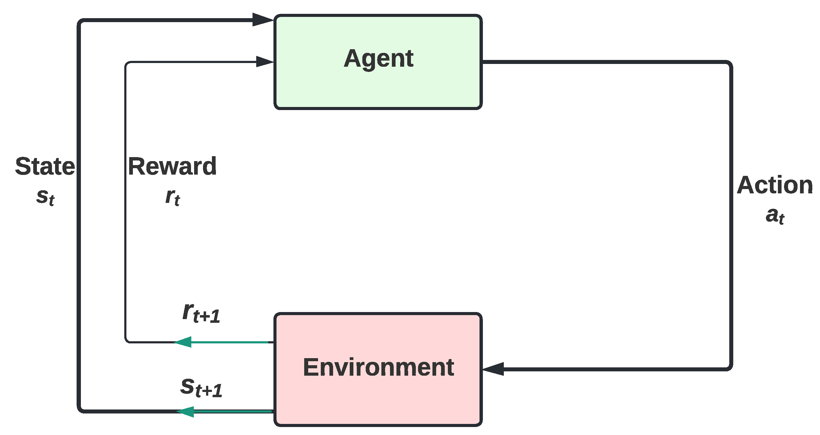
Figure 1. Reinforcement learning algorithm flowchart.
Drones 07 00123 g001
Figure 2. Big picture UAV path over buildings.
Drones 07 00123 g002
Figure 3. Big picture UAV path around buildings.
Drones 07 00123 g003
Figure 4. Q-learning processing scheme during the UAV journey.
Drones 07 00123 g004
Figure 5. UAV movement space in the scenery.
Drones 07 00123 g005
Figure 6. Power consumption based on wind speed and distance traveled.
Drones 07 00123 g006
Figure 7. Cross-checking RL parameters for 1000 samples.
Drones 07 00123 g007
Figure 8. Convergence Analysis by UAV distance traveled.
Drones 07 00123 g008
Figure 9. Convergence Analysis by UAV distance traveled.
Drones 07 00123 g009
Figure 10. Convergence Analysis by UAV distance traveled.
Drones 07 00123 g010
Figure 11. Convergence Analysis by UAV distance traveled.
Drones 07 00123 g011
Figure 12. Convergence Analysis by UAV distance traveled.
Drones 07 00123 g012
Figure 13. Convergence Analysis by UAV distance traveled.
Drones 07 00123 g013
Figure 14. Stockholm optical link topology.
Drones 07 00123 g014
Figure 15. Average wind speed variation for each UAV during the mission.
Drones 07 00123 g015
Figure 16. Average wind speed variation for each UAV during the mission.
Drones 07 00123 g016
Figure 17. Distance traveled by each UAV during the mission.
Drones 07 00123 g017
Figure 18. Power consumption by each UAV during the mission.
Drones 07 00123 g018
Table 1. Roughness factor by land cover types [71].
Roughness Length z 0 Land Cover Types
0.0002 mWater surfaces: seas and Lakes
0.0024 mOpen terrain with smooth surface,
e.g., concrete, airport runways, mown grass, etc.
0.03 mOpen agricultural land without
fences and hedges; maybe some far
apart buildings and very gentle hills
0.055 mAgricultural land with a few buildings
and 8 m high hedges separated by more than 1 km
0.1 mAgricultural land with a few buildings and 8 m
high hedges seperated by approx. 500 m
0.2 mAgricultural land with many trees, bushes, and
plants, or 8 m high hedges separated by approx. 250 m
0.4 mTowns, villages, agricultural land with many
or high hedges, forests and very rough and uneven terrain
0.6 mLarge towns with high buildings
1.6 mLarge cities with high buildings and skyscrapers
Table 2. Configuration of the test experiments.
ExperimentNumber of ObstacleArrangement of High Wind
Speed Points in the Scenario
11Randomly
22Randomly
39Randomly
449 (in the center)In the center
549 (in the center)in the upper half
Table 3. Simulation parameters.
ParameterValue
Total Payload90 kg [32]
UAV speed15 m/s
Number of UAVs15
Maximum distance between UAVs aerial links2 km
Number of Resource stations4
Maximum wind speed13 m/s
Minimum wind speed6 m/s
Minimum height of obstacles30 m
Maximum height of obstacles121 m
Gravity acceleration (g)9.8 m/s [74,75,76]
Maximum exploration rate ( m a x ϵ )1
Minimum exploration rate ( m i n ϵ )0
Roughness factor( z 0 )1.6 m
Initial wind speed ( v 1 )5 m/s
Initial altitude the speed ( h 2 )8.5 m
Exploration decay rate0.01
Disclaimer/Publisher’s Note: The statements, opinions and data contained in all publications are solely those of the individual author(s) and contributor(s) and not of MDPI and/or the editor(s). MDPI and/or the editor(s) disclaim responsibility for any injury to people or property resulting from any ideas, methods, instructions or products referred to in the content.