Abstract
In the last decade, small unmanned aerial vehicles (UAVs/drones) have become increasingly popular in the airborne observation of large areas for many purposes, such as the monitoring of agricultural areas, the tracking of wild animals in their natural habitats, and the counting of livestock. Coupled with deep learning, they allow for automatic image processing and recognition. The aim of this work was to detect and count the deer population in northwestern Serbia from such images using deep neural networks, a tedious process that otherwise requires a lot of time and effort. In this paper, we present and compare the performance of several state-of-the-art network architectures, trained on a manually annotated set of images, and use it to predict the presence of objects in the rest of the dataset. We implemented three versions of the You Only Look Once (YOLO) architecture and a Single Shot Multibox Detector (SSD) to detect deer in a dense forest environment and measured their performance based on mean average precision (mAP), precision, recall, and F1 score. Moreover, we also evaluated the models based on their real-time performance. The results showed that the selected models were able to detect deer with a mean average precision of up to 70.45% and a confidence score of up to a 99%. The highest precision was achieved by the fourth version of YOLO with 86%, as well as the highest recall value of 75%. Its compressed version achieved slightly lower results, with 83% mAP in its best case, but it demonstrated four times better real-time performance. The counting function was applied on the best-performing models, providing us with the exact distribution of deer over all images. Yolov4 obtained an error of 8.3% in counting, while Yolov4-tiny mistook 12 deer, which accounted for an error of 7.1%.
1. Introduction
The world’s growing population and the expanding region of human habitation have changed the natural life populace and behavior. Many wild animals are forced to migrate and re-adapt in order to survive, and monitoring has become an essential task in ecosystem preservation. Identifying and counting animals is traditionally carried out manually, using methods such as surveys from manned aircraft, the analysis of camera footage, and other manual techniques. Recent developments in technology have made UAVs increasingly affordable and effective, allowing us to quickly obtain large amounts of aerial data at a high resolution. Parallel to this, the progress in object detection algorithms and computational power has allowed us to process images in a fast and accurate manner. The detection of animals in aerial images serves many purposes, such as:
- Censuses: authorities need to periodically obtain animal counts to monitor the health of the animals in wildlife parks, game centers, hunting grounds, etc. [1,2];
- Poaching prevention: many studies have been conducted on monitoring endangered species. Thousands of elephants, rhinos, etc., are poached every year in Africa, even to this day [3];
- Minimization of human interference: the prevention of accidents and damage from conflicts between humans and animals in border regions;
- Livestock monitoring: the automation of livestock counting for the monitoring of farm production [4].
To better understand the importance of these tasks, let us observe the last point: the most common and redundant job of a rancher or herdsman is counting their herd to derive a headcount. It is a job that is frequently required and naturally takes up a large amount of the rancher’s time. If we could somehow automate that process, we would save not only a lot of time for that rancher, but also a lot of money. A good example is sheep export from Australia, as explained in [5]. Exporters receive about AUD 80 for each sheep counted at its overseas destination, and hence lose this amount for every sheep that is delivered overseas but not counted by an overseas tally clerk. This loss is estimated to be about 3% of the sheep exported, suggesting that about 15,000 sheep are shipped each year that are not counted overseas. This amounts to an annual loss to the industry of about AUD 1,200,000. However, for an automated counting system to be adopted by an industry, it must be at least as accurate as, and preferably faster and less expensive than, the manual system it replaces. In this paper, we describe one approach to monitoring wild animals, which is the application of deep learning methods to UAV images. More specifically, we observed a deer population in a dense forest environment. The goal of this project was to compare models that can detect extremely small objects with a high mean average precision and, at the same time, demonstrate competitive real-time performance.
The main goal of this work was to automate the process of counting deer near Plavna, a hunting ground in northwestern Serbia. According to the Serbian Law of Wildlife and Hunting, an optimal number of deer must be preserved at all times; hence, the counting must be performed twice per year. So far, the counting process has been carried out manually, which requires a lot of human power directly in the field and a large amount of time. Other than that, it poses a risk for humans of getting close to the animals; it is expensive; and, most importantly, it lacks accuracy. To offer a more efficient system, in this paper, we propose a pipeline for animal (object) detection based on convolutional neural networks (CNNs) applied to UAV images and evaluate the current state-of-the-art models, including YOLOv3, YOLOv4, YOLOv4-tiny, and SSD. Figure 1 depicts an overall methodology flowchart for this study. To summarize, the detection of animals in the environment should give an insight into the location and distribution of animals at a particular location, as well as their approximate number over the observed area. The fourth version of YOLO made a remarkable improvement in small object detection [6,7,8,9], so we set YOLOv4 as the benchmark.
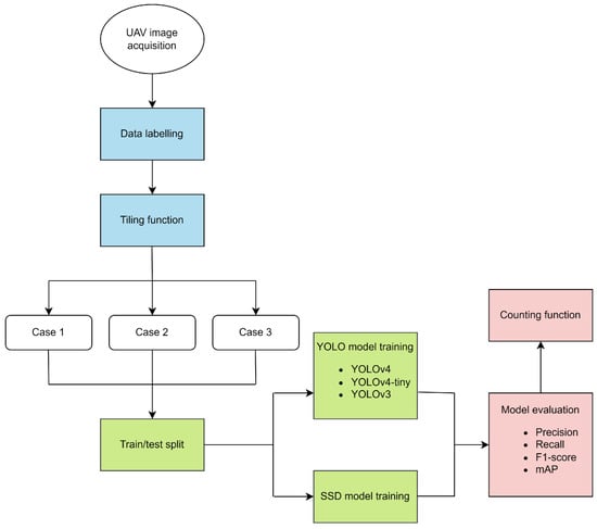
Figure 1.
Methodology flowchart of this study. Blue parts represent data preprocessing, green parts concern AI (artificial intelligence) model training, and red parts indicate the evaluation of the results using four metrics and a counting function.
As mentioned already, these models were applied to UAV images obtained over an area in northwestern Serbia. A UAV, more commonly known as a drone, is an aircraft without any human pilot, i.e., they are capable of flying autonomously. These vehicles follow flight plans based on GPS coordinates, which are usually programmed before the flight but can also be changed during the flight. A University of Adelaide study has shown that monitoring wildlife using drones is more accurate than traditional counting approaches. In the Epic Duck Challenge, teams experimented on semi-automating the counting process by making fake bird colonies out of decoy ducks on a beach in Adelaide, Australia, and developing an algorithm to count the birds. They found that the computer was able to produce a count similar to that of a human reviewing the scene. These studies have opened up the potential of drones to not only save time but also to increase the accuracy of the data that are collected.
Moreover, many previous studies have demonstrated the success of using CNNs to detect animals from UAV or similar images. Recent important works have considered the detection of large mammals in the African Savanna. Duporge et al. [10] employed artificial neural networks for high-resolution satellite imagery to automatically detect and count African elephants in a woodland savanna ecosystem. These censuses play an important part in the fight against the extinction of many endangered species in Africa, which is why much more research has been conducted. In [3], the authors proposed several recommendations to guide CNN models for the detection of large mammals in UAV images consisting mostly of the background class. Similarly, the authors of [11] proposed the novel Context-aware Dense Feature Distillation (CDFD) method, addressing the difficulty of detecting small objects in remote-sensing images and focused on improving remote-sensing object detection performance. YOLO models have proved to be highly successful in animal detection when trained on high-quality datasets and properly optimized for the task at hand. Some results can be found in [12,13]. Han et al. implemented the YOLOv3 network, achieving over 95% accuracy in detecting livestock in grassland. Gomez et al. demonstrated the efficiency of the YOLOv4 model even when training on low-quality images while addressing the issue of monitoring animals in the wild without disturbing them.
Another frequently analyzed problem is cattle counting, which can be of great importance for trade and the economies of many countries. Several detectors can be found in the works of Chamoso et al. [1] and van Gemert et al. [4], both tackling the problem of cattle counting. Moreover, the Verschoor Aerial Cow Dataset [14], a dataset available to the public, allows for more research to to be carried out on animal monitoring. This dataset contains recordings of cows in a meadow, captured with a GoPro HERO 3 camera attached to a UAV. It also includes labels with the location of the cows in each video frame. As usual, the location of each cow is denoted by a bounding box surrounding the object. Using drones in combination with AI models for animal detection is a relatively new field of research with many potential applications in wildlife conservation and monitoring. During our research, we encountered this topic in several studies, which included using AI models with thermal and regular camera images [5,7,15], video footage [9], and satellite imagery [10]. Still, there is a major gap in the research regarding the use of drones for animal detection due to the limited availability of high-quality data for training, the issue we address in Section 5.1. However, it is important to note the importance of the safe use of UAV aircraft around rural areas where there exist security threats to people, objects, and country regulations [16].
2. Object Detection Techniques
In addition to detecting the presence of animals, in order to effectively track them and monitor their actions, it is also necessary to localize the animals within the image. This is the task of object detection. Object detection systems locate all positions of objects of interest in the input by framing them into bounding boxes and classifying them into categories. The process consists of two or three steps: localization—the drawing of bounding boxes; the extraction of features for each region; and recognition—identifying the classes of the objects in the image. In our case, we dealt with only one class—deer. A modern detector usually consists of two main parts—the backbone and the head of the detector [17]. The backbone refers to the feature extractor network and is a crucial part of every CNN. It takes an input image and extracts the feature map upon which the rest of the network is based. Depending on the platform that the detector runs on (CPU or GPU), the backbone varies mostly between VGG, ResNet, DenseNet, and MobileNet [18]. There are two approaches for the development of the head of the detector—an approach based on the region proposal algorithms, also known as a two-stage approach, and an approach based on regression or classification that uses real-time and unified networks, i.e., the one-stage approach. In this work, we focused on the one-stage approach. There were two main factors contributing to this decision:
- Speed: One-stage detectors are typically faster than two-stage detectors as they perform all the necessary operations, including object detection and classification, in a single pass through the network. This makes them well-suited for real-time applications such as ours.
- Simplicity: One-stage detectors are generally simpler and require less computational power. Due to our limited resources during this research, they were a better solution.
2.1. You Only Look Once
As a very simple and extremely fast model, this state-of-the-art algorithm gained popularity soon after it was first presented in 2015 [19]. It reframed object detection as a single regression problem, progressing straight from image pixels to bounding box coordinates and class probabilities. As a regression problem, it divides the input image into an S × S grid and, if the center of the object falls within the target grid cell, this grid is responsible for detecting the object by predicting the B bounding boxes, the confidence score, and the class probability. Each bounding box consists of four predictions: x y, w, and h. The (x,y) coordinates represent the center coordinates of the predicted bounding box, relative to the boundaries of the grid cell. The remaining two coordinates are the width and height, respectively, and they are predicted relative to the whole image. The confidence score represents how confident the model is that the specific bounding box contains the object. It is expressed as the accuracy, and, naturally, if there is no object in that cell, the confidence score is equal to zero.
All versions of YOLO use extensive data augmentation, divided into photometric distortions and geometric distortions. In dealing with photometric distortions, the brightness, contrast, hue, saturation, and noise of an image are adjusted. For geometric distortions, random scaling, cropping, flipping, and rotating are performed. In YOLOv4, the authors also introduced a new method of mosaic data augmentation. Mosaic data augmentation is performed by mixing four training images, in contrast with the already known CutMix process [20], which mixes only two input images. In this way, batch normalization calculates activation statistics from four different images on each layer, which significantly reduces the need for a large mini-batch size.
In our work, the pre-trained YOLOv4 model was further trained using images with dimensions of 416 × 416. The learning rate was initialized to 0.001 with a decay rate of 0.0005, and the momentum was set to 0.9. The training was carried out in 2000 steps with a batch size of 64. During the training of YOLOv4, firstly, the size of the input images was adjusted so that all the input images had the same fixed size. We also trained YOLOv4-tiny, which is a lightweight YOLO-series method, representing the compressed version of YOLOv4. Lightweight methods such as this have a simpler network structure and fewer parameters than other networks. Therefore, they require lower computational resources and memory and have a higher detection speed. The prediction process is completely the same as that in YOLOv3 and YOLOv4, but significantly faster. The frames per second (FPS) in YOLOv4-tiny is approximated to be eight times lower than in YOLOv4, while the accuracy for YOLOv4-tiny is two thirds that of YOLOv4. Hence, for real-time object detection problems, the compressed version is preferred.
2.2. Single Shot Multibox Detector
SSD is a method introduced by Liu et al. [21] for detecting objects in images using a single deep neural network, i.e., a one-stage detector. The SSD approach is based on a feed-forward convolutional network that produces a fixed-size collection of bounding boxes and a measurement of certainty that the objects are in those boxes, followed by a non-maximum suppression (NMS) step to produce the final detection. According to the authors, SSD is much faster than other well-known object detectors, such as YOLO and Faster-RCNN, while maintaining the same accuracy. We confirmed this in our research, as SSD finished training in 5000 steps, approximately three times faster than YOLO versions 3 and 4. However, the performance was slightly lower than what YOLO achieved.
The SSD model can be divided into three parts: the base network, auxiliary network, and prediction network. The base of SSD is any image classification network without the last fully connected layer, and it is used to extract a feature map from the input image. This feature map is then passed through an auxiliary network. We used a model with MobileNet as its base. The key idea underlying SSD is the concept of default boxes, which represent the careful selection of bounding boxes based on their sizes, aspect ratios, and positions across the image. There are 8732 default bounding boxes. The network is trained to perform two main tasks: (1) classifying which amongst the 8732 default boxes are positive; (2) predicting offsets from the positive default box coordinates to obtain the final predicted bounding boxes. During the training, each ground truth box is matched to the default box with the best Jaccard overlap (J), with a threshold of 0.5. The Jaccard coefficient measures the similarity between finite sample sets and is defined as the size of the intersection divided by the size of the union of the sample sets (A is set 1 and B is set 2):
The output of the detector head is the number of predicted bounding boxes overlapping each other for the same ground truth. Before the final prediction is generated, the overlapped bounding boxes need to be processed and filtered. SSD uses non-maximum suppression to remove duplicate predictions pointing to the same object. NMS is an essential method for postprocessing in object detection to eliminate the redundant bounding boxes. This is carried out by sorting the predictions by the confidence score.
The overall objective loss function is the weighted sum of the localization loss and the confidence loss [21]:
where N is the number of matched default boxes, and and are the confidence and localization loss, respectively. If there are no matched boxes, i.e., N = 0, then the loss equals 0. The localization loss is a smooth loss between the predicted box l and the ground truth box g. The confidence loss is the softmax loss over multiple class confidences c. We calculated and present the graphs of all of these losses for our training in the Results section.
We used the TensorFlow Object Detection API (application programming interface) [22] to build the SSD model. This API allows the implementations of different deep learning object detection algorithms, from which we selected the model referred to as COCO, which has an SSD300 architecture and was pre-trained on the COCO dataset [23]. The reason behind this decision was that objects in COCO tend to be smaller than in other frequently used datasets, such as PASCAL VOC [24], and it contains images with an input size of 300 × 300, which made it suitable for our specific problem. The pre-trained model was trained at a learning rate of for the first 160,000 iterations, which was then decreased to for the next 40,000 iterations, and further down to for another 40,000 iterations. We used default hyperparameter values for this model, as retrieved from the API.
SSD also includes data augmentation in order to make the model more robust to various input object sizes and shapes. Each image is first randomly sampled by taking either the patch of the image with the specified minimum Jaccard overlap with the object of interest, or the entire image. After that, each sampled patch is resized to a fixed size and is flipped horizontally with a probability of 0.5, in addition to applying some photo-metric distortions, such as random brightness, contrast, hue, and saturation [21].
3. Materials and Methods
3.1. Data
Aerial imaging provides a detailed overview and quick monitoring of large areas, making it a very efficient way to solve this specific problem. As mentioned in Section 1, the data were collected in the northwestern region of Serbia. The hunting ground of Plavna covers a total of 2619 ha, of which 630 ha are enclosed. The predominant large species are deer and wild boar. The dataset consisted of 30 UAV images, with three different image sizes, originating from three different UAVs: 4608 × 3456 (DJI Phantom 4 Pro V2.0), 4864 × 3648 (Parrot Company SenseFly eBee), and 4000 × 3000 pixels (DJI Inspire 1), whose specifications are shown in Figure 2.
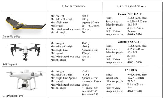
Figure 2.
UAV performances and camera specifications of platforms used for data acquisitions.
The number of images of each size is provided in Table 1. As part of the data augmentation and a method for model evaluation, we divided all images into smaller pieces. We achieved this by applying the tiling function on each image of our dataset. Each smaller image was 416 × 416 × 3 in size, and all the deer were labeled manually. After applying the tiling function to these 30 images, 2340 new smaller images were obtained, of which 120 contained ground truth, i.e., bounding boxes. There were a total of 169 objects (deer) or regions of interest (ROIs) in the complete dataset.

Table 1.
Details of the images provided and the number of labels.
3.2. Ground Truth
All the tested models required only bounding boxes for the objects as labels for training. So, before training any detection network, the manual task of annotating all training images had to be performed to acquire ground truth. The process of labeling involved visual scanning and marking the parts of the images where the objects of interest were located. As mentioned, 169 deer were identified in the dataset; hence, 169 bounding boxes were drawn. For this purpose, the LabelImg annotation tool [25] was used. This graphical image annotation tool was written in Python and allows for the labeling of images with minimum effort. During the labeling process, bounding boxes were drawn around each deer in the image. Figure 3 shows the LabelImg interface for one image from our dataset.
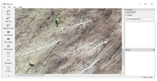
Figure 3.
Labeling with LabelImg tool.
The information provided for the bounding box also depends on the output format, i.e., on the network requirements. Pascal VOC is the format used by the Pascal VOC dataset (Figure 4). These kinds of annotation are needed to train the Single Shot Multibox Detector. After completing the annotation, an xml file is generated for each image annotated. The coordinates of each bounding box in that file are encoded with four values expressed as pixel locations: , where are the coordinates of the top-left corner of the bounding box and are the coordinates of the bottom-right corner of the bounding box. Besides these coordinates, the path to the file is provided, along with the class name, image size, and image depth.
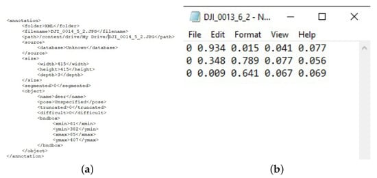
Figure 4.
Annotations generated by LabelImg tool. (a) Annotation in Pascal VOC format. (b) Annotation in YOLO format.
The Yolo format is used for training all versions of the You Only Look Once networks. As in the previous case, a new file is generated for every image, but this time in the txt format. This text file contains as many rows as there are objects of interest in that image, i.e, one row for each deer in our case. Each of these rows contains the class number, ranging from 0 up to the number of classes, and the corresponding bounding box coordinates. Since there was only one class in our dataset, the first element of each row was 0. Furthermore, the bounding box is represented by four values: , where are the coordinates of the central pixel of the bounding box, and w and h represent the width and height of that bounding box. Moreover, all of these values are normalized, i.e., the value of x is divided by the width of the entire image and the value of y by its height.
3.3. Methods
To overcome the problem of small objects on a large background, we applied the tiling function as part of the preprocessing. This function divides each image into smaller pieces of the same size. It is common practice to split up large images into smaller tiles and assess each one individually. E.g., given an image 4000 × 3000 pixels in size, as was the case for some of our images, if we assume a tile size of 1000 × 1000 pixels as a realistic size for naked-eye screening, we would have to divide such an image into 12 smaller pieces. The main idea behind this approach is to break down a large image into smaller, manageable chunks, which can be further processed by the AI model separately and then combined to produce a final output. There are several ways of dividing large images into smaller pieces, such as using a sliding window or a fixed grid. In our work, we decided on the latter in order to obtain non-overlapping tiles. This was carried out by specifying a fixed size for the patches, as models require the same input size for all images, and then dividing each image. Object detection was then performed on each patch separately. By utilizing this approach, we not only generated more images for our training, but the models were allowed to focus on a specific region of the image, which could improve the accuracy and efficiency of the analysis. Additionally, breaking down the image into smaller pieces could also help reduce the amount of memory and computational resources required to process the image, which could be particularly important when working with large or high-resolution images. Moreover, in this way, we reduced the amount of background class in each image, performed data augmentation, and resized all images to the same size. We also tested the performance on different numbers of tiles and showed that all models performed poorly when dealing with a large class imbalance. As we set YOLOv4 as our benchmark, all images were divided into smaller pieces 416 × 416 pixels in size, in order to better match this model’s requirements.
We compared the results of each model using three problem setups:
- The training set contained only positive samples;
- The training set contained an equal number of positive and negative samples;
- The training set contained substantially more negative samples.
For the positive samples, the fixed amount was determined by the size of the labeled dataset. The positive samples dataset contained 120 tiles (Figure 5), that is, there were 120 images in the first case. In the second case, there were 120 images for positive samples and 120 random negative samples (Figure 6), chosen in such a way that the number of positive and negative sample tiles from each image was the same. The number of negative samples in the third case was substantially larger, with 2220 tiles containing no animals, summing up to 2340 images in total. The annotation file in the case of the negative samples was an empty txt or xml file.
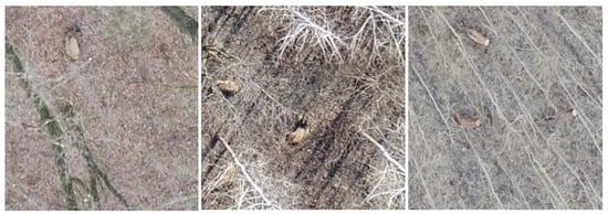
Figure 5.
Examples of positive samples, i.e., tiles containing at least one deer.
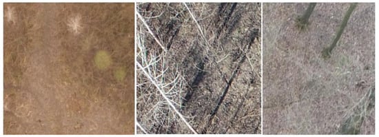
Figure 6.
Examples of negative samples, i.e., tiles without deer.
The idea for such an evaluation method came from the authors of YOLO, who proposed that in order to increase the precision of the network, there should be as many images of negative samples as there are images with objects. We checked this statement by training in all three cases. The results achieved were different for all the models.
The experimental setups of some hyperparameters are illustrated in Table 2. These parameters were the same for all three cases.
Table 2.
Configuration of hyperparameters of each model.
YOLOv4 consists of four blocks—a CSPDarknet53 backbone [26], an SPP additional module [27], a PANet path-aggregation neck [28], and a YOLOv3 [19] (anchor-based) head. The described architecture was first pre-trained on ImageNet [29]. In the network, the maximum pooling filter was applied three times, with one stride and sizes of 5, 9, and 13, in this particular order. On the other hand, no pooling layer was implemented in YOLOv3. In the compressed YOLOv4, this type of layer was used consistently, after every four convolutional layers, with both a size and a stride of 2. The main difference between YOLOv4 and YOLOv4-tiny is that the network size is dramatically reduced in the latter. Moreover, the number of convolutional layers in the CSP backbone is compressed: it uses a CSPDarknet53-tiny backbone network instead of the CSPDarknet53 backbone used in YOLOv4, which contains fewer convolution layers. Is also contains only two YOLO heads, as opposed to the three in YOLOv4. Beside heads, the complete network contains 21 convolutional layers (as opposed to the 110 layers used in YOLO4 and 75 used in YOLOv3), as well as 3 pooling layers. To further simplify the computation process, the YOLOv4-tiny method uses the LeakyReLU function as an activation function in the CSPDarknet53-tiny network instead of the Mish activation function, except for the convolutional layers which come before the head layers.
To train these models, first we had to clone the darknet github repository [30] and initialize the weights with the pre-trained weights, which were different and specialized for each model. These weights can also be obtained from [30]. To set up the number of training steps, we followed the authors’ recommendations for the repository. The number of steps was equal to the number of classes multiplied by 2000; thus, as we had only one class, we trained for 2000 steps. Further fine-tuning was required in order to adapt the model to the different datasets. The number of filters used before each YOLO layer was calculated as , so we changed all the filter values to 18 if the neural network layer preceded a “YOLO” layer. The authors also provided further recommendations on how to improve the training precision and speed by adjusting the network resolution. After increasing the network resolution, i.e., increasing the tile size, we compared the performance of YOLOv4-tiny for images of three different sizes: 416 × 416, 512 × 512, and 608 × 608. SSD was trained on the same dataset for 5000, 7000, and 9000 iterations to compare the performances. In all cases, the learning rate was , without decay. The architecture of both networks is shown in Figure 7.
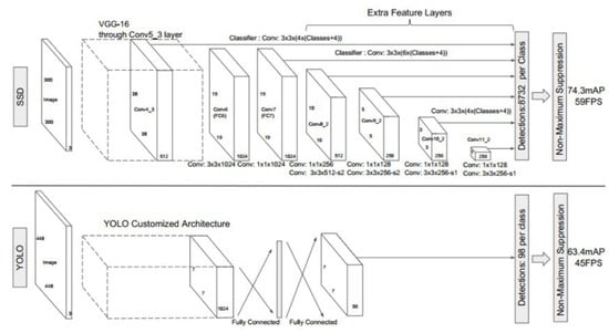
Figure 7.
A comparison between the SSD and YOLO network architectures [21]. The architecture of YOLO uses an intermediate fully connected layer instead of the convolutional filter used in SSD for the final predictions.
3.4. Evaluation Metrics
For the purpose of estimating the performance of the predictions, several concepts are introduced below. In the case of object detection, the evaluation metrics employed measured how close the detected bounding boxes were to the ground truth bounding boxes. This is called Intersection Over Union (IOU), and it was measured by assessing the overlap of the two bounding boxes. We distinguished three different sizes of bounding boxes: small (area pixels), medium ( area pixels), and large (area ). As each model used annotations in a specific format, their results were dependent on the specific metric implementation associated with the dataset on which they were pre-trained. This meant that the evaluation metrics were directly associated with a given annotation format; therefore, the results are reported only for the metrics implemented for the benchmarking dataset. Table 3 lists the object detection methods that we used, along with the metrics used to report their results. The metrics have the following notations:
Table 3.
Object detection methods used and their performance metrics.
- mAP—mean average precision over classes averaged over IOU thresholds ranging from .5 to .95 with .05 increments;
- mAP@.50, mAP@.75—mean average precision at 50% and 75% IOU, respectively;
- APS, APM, APL—mean average precision for small, medium, and large objects, respectively;
- AR1, AR10, AR100—average recall with at most 1, 10, and 100 detections per image, respectively;
- ARS, ARM, ARL—average recall with at most 100 detections per image for small, medium, and large objects, respectively. These three metrics are referred to as AP across scale.
During the detection, there were four possible outcomes: true positive, true negative, false positive (FP), and false negative (FN), which we denote with , and , respectively. True positive (TP) refers to a correct prediction with an IOU larger than or equal to a certain threshold. Conversely, true negative (TN) refers to a true detection that has an IOU smaller than the threshold. False positives happen when a section of the image is recognized as a deer but is actually part of the background. This can occur when items in the background, such as logs or large rocks, are mistaken for animals due to the similarity in color and size. False negatives happen when deer are in the image but are not recognized by the detector.
Precision is the ability of a model to identify only relevant objects. It denotes the percentage of correct positive predictions, while recall is defined by the ratio of the positive instances that are correctly detected by the detector and all labeled positive instances. The precision and recall were calculated as follows:
There is a trade-off between precision and recall, meaning that as the precision curve increases, the recall value decreases, and vice versa. However, the two do not encapsulate the whole picture. Instead, we used mean average precision and recall values. MAP was calculated by the mean of the average precision for all classes, that is:
where is the average precision for class i, and C is the total number of classes in the dataset. The complete calculation for the average precision can be found in [31].
The F1 measure indicates the trade-off between recall and precision, as shown in the equation below.
The F1 score is limited to a [0, 1] interval, with a value of 0 if either the precision or recall (or both) are 0, and a value of 1 when both precision and recall are 1.
4. Results
The best results for each model are shown in Table 4. All tested methods were implemented in Google Colaboratory, with the use of GPU and CUDA, for a higher training speed. The bounding boxes of each deer detected in the frames were annotated with a confidence score and the class name.
Table 4.
Comparison of the best results achieved by each model and the case in which they were achieved.
Before training, the dataset is split into the training and test set for performance evaluation, with train and test sets containing 85% and 15% of all images, respectively. This division is performed randomly, using the implemented function. The number of images in each set depends on which of the three setups is examined. All models are fed with the same size input data—416 × 416, which is required for You Only Look Once models. SSD, however, uses images of size 300 × 300, but resizing is carried out automatically by the model itself. For the comparison of models we used two performance evaluation metrics—mean average precision (with IOU = 0.5) and recall. We also used precision, as well as F1 score for comparison between different YOLO models.
According to the overall detection results for each model in their best case presented in Table 4, the two versions of YOLOv4 outperformed the YOLOv3 approach by 27–32% in terms of mean average precision.The results obtained for YOLOv3 were not favorable, with only 29.8% mAP and 0.30 recall in the first case and 38.38% mAP and 0.25 recall in the second case. Specifically, YOLOv4, with the CSPDarknet53 backbone, achieved the top mAP in all three cases of all YOLO models examined. In comparison, the Darknet-53 backbone obtained only 38.38% mAP as the best result. On the other hand, YOLOv4 had a competitive recall performance, whereas SSD achieved a poor recall value in all three cases.
Next, we observed how the SSD network performed with more steps, as we noticed that the mAP value was very unstable in the early steps and became more stable after the 3000th step. For this reason, we trained using three cases, starting from 5000 steps and increasing by 2000 for each subsequent training process. There was a steady increase in the mAP value from approximately the 2000th step until the 5000th, after which the curve started to converge, i.e., more training was unlikely to lead to model improvement, so we deduced that 5000 steps was an optimal value and used it for further training. These values are shown in Figure 8. For this evaluation, mean average precision was used with an IOU of 50%.
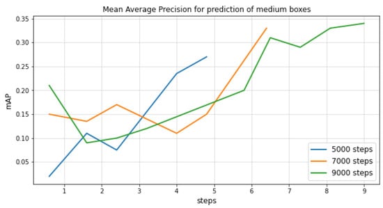
Figure 8.
mAP@.50 IOU curves for different numbers of training steps for the Single Shot Detector.
However, when we set the threshold of IOU to 0.75, that is, when we chose a more restrictive IOU, the mAP value significantly improved with a higher number of steps. This is shown in Figure 9, which shows that adding more steps for the training increased the mAP by up to 10% from 5000 to 9000 steps for the detection of medium-sized boxes. Since the main goal of this work was the counting of deer, and not strictly localizing them, we decided that IOU = 0.50 was sufficient for this specific problem.
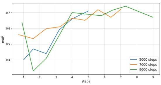
Figure 9.
mAP@.75 IOU curves for different numbers of training steps for the Single Shot Detector.
Based on research using the VOC2017 test set, the authors of [21] deduced that SSD performed much worse on smaller objects than on larger ones and was very sensitive to the bounding box size. Our mAP and recall results for the detection of small and medium objects confirmed this statement. Several comparisons of the detection results between different models are visualized in Figure 10 and Figure 11. As shown in Figure 10, the confidence scores of the predictions from both YOLOv4 and SSD were very high. However, in Figure 11, we can see that YOLOv4-tiny predicted the same deer with a much lower confidence score than YOLOv4 and SSD; however, on the contrary, it provided a very high confidence score for small target objects. When it came to real-time performance, YOLOv4-tiny was significantly faster than all the other trained models—up to four times faster than YOLOv4 and v3 and two times faster than SSD.
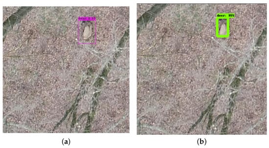
Figure 10.
Confidence score of YOLOv4 (a) and SSD (b) on the same image. (a) You Only Look Once version 4. (b) Single Shot Multibox Detector.
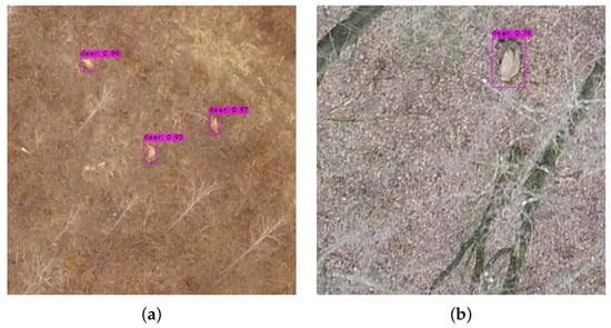
Figure 11.
Comparison of YOLOv4-tiny performance for detecting small (a) and medium objects (b).
4.1. SSD Results
To train an intelligent object detection model with good performance, it is crucial to provide enough samples for it to learn the general patterns. That is why usually, the more data one has, the better the results achieved. For SSD, the third case yielded the best results, while the first case, in which we trained the model using only 102 images, yielded the smallest mAP but the highest recall.
We trained the SSD model in all three setups for 5000 steps and noticed a steady increase of 5% for each case with more images. That is, in the first case, the maximum mAP rate achieved was 60%; in the second case, with double the number of images, the mAP was around 65%; and in the third case, the highest mAP was 70%. The results for the first and third cases are shown in Figure 12, while the results for the second case can be seen in Figure 13 and Figure 14. The total loss also followed this trend and was much lower in the third case. What is more, the loss started to increase with the number of steps in setups 1 and 2, while in the third setup it showed the opposite trend and constantly declined. Given that the third case yielded the best results, we also show the classification and localization loss results for this case in Figure 15.
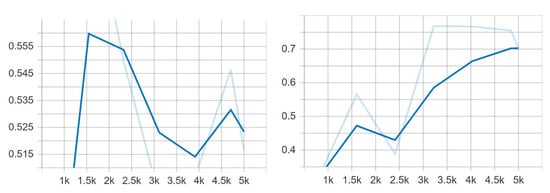
Figure 12.
mAP@.50 IOU—the average precision using IOU = 0.5 for the first case (left) and the third case (right).
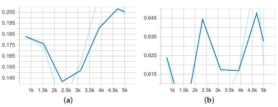
Figure 13.
Mean average precision for small and medium objects when trained on the set of 240 images, of which 120 were positive and 120 negative samples. (a) Detection of small objects. (b) Detection of medium objects.
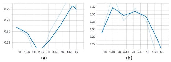
Figure 14.
Mean average recall for detecting small and medium bounding boxes from 240 images after 5000 steps of training. (a) Detection of small objects. (b) Detection of medium objects.
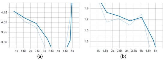
Figure 15.
Classification and localization loss of the SSD model trained on 1989 images for 5000 steps. (a) Classification loss. (b) Localization loss.
4.2. YOLO Results
After training each model for 2000 steps with the hyperparameters listed in Table 2, YOLOv4 achieved a better performance than both YOLOv3 and YOLOv4-tiny in all three cases based on each of the four measurements, with more than two times better results than YOLOv3 and slightly better results than YOLOv4-tiny. In contrast to YOLOv4, the tiny version worked the best in the first case when trained only on positive samples, achieving an mAP of 65.11% and a precision of 0.79. The performances of the first, second, and third case are presented in Table 5, Table 6 and Table 7.
Table 5.
Results achieved by all the models in the first case.
Table 6.
Results achieved by all the models in the second case.
Table 7.
Results achieved by all the models in the third case.
For the purpose of counting the number of detected deer, we tested all of the images at once, both training and testing, and saved the output as a text file. As already mentioned, the number of manually annotated bounding boxes was 169, i.e., a human could find 169 deer in the given dataset. In contrast, our model with the highest mAP—YOLOv4 in the second case—recorded 155 deer in total, while the compressed version found 157 deer in all the images.
4.3. Generalization and False Positive Results
According to the authors of [21], SSD may encounter higher confusion between classes with similar object categories, especially for animals. On the other hand, in [17], it is claimed that YOLOv4 is invariant to background changes and deals better with recognizing objects in new environments compared to the other detectors. Moreover, YOLO learns the general representations of objects, so it is much less likely to make errors when applied to new domains or unexpected inputs. We tested both of these statements by adding new images to our testing set that contained other animals of similar sizes and colors to our deer class. Images from the Verschoor Aerial Cow Dataset mentioned in Section 1, as well as some images from the internet, which were labeled for reuse, were used to test the generality of the CNN in a broader scope of image conditions. We used the trained algorithms as-is and only applied them on novel test images. We confirmed the invariance of YOLOv4 to differences in the background but not to different animal species. This model was able to successfully recognize the deer class in all additional images, despite a large difference in the background. However, it mistook other animals for deer, e.g., cows and elephants. For our purposes of counting deer in hunting ground areas where there are no other classes of animals, this did not represent much of a problem, as both YOLOv4 and YOLOv4-tiny were able to successfully detect almost all deer in the images. We therefore concluded that the algorithms developed in this work could be applied in other settings, i.e., for the detection of other animal species and in variable background scenes. For example, YOLOv4 detected almost every cow from the Verschoor Aerial Cow Dataset despite a large change in the background from shades of gray in the forest environment to green meadows. A few characteristic examples are presented in Figure 16.
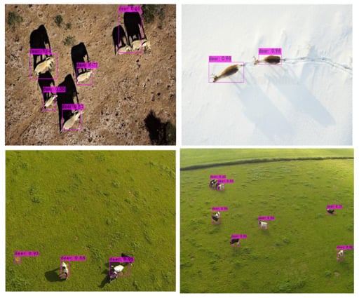
Figure 16.
Results of YOLOv4 when applied to new images with different backgrounds to those in the training set.
5. Discussion
After observing the results for the SSD in all three cases, we determined that the best performance was achieved in the third case, with the most data available. The explanation for why the SSD performed much better in the third case, especially compared to the other models, lay in the use of hard negative mining. When the default box system was used in the SSD, the number of negative matches was much larger than the number of positive matches. In this case, we trained the model to learn the background space rather than detect objects, and this impeded the training. To overcome this, instead of using all the negatives, the SSD sorted these negatives by their calculated confidence loss and then picked the negatives with the highest loss and made sure that the ratio between the selected negatives and positives was at most 3:1. This led to faster and more stable training, as well as a lower class imbalance.
In the case of YOLOv4, the best results were achieved in the second case, as suggested by the authors of that model, who inspired the idea for the three evaluation cases by stating that the optimal situation was for the model to have as many negative samples as positive. YOLOv4 performed slightly better in the second case, with a 1.24% higher mAP and a 3% better precision. Although the difference was not significantly large, our model was trained on only 2000 steps. We suspect that the difference would be higher for a higher number of classes and, therefore, more training steps. The changes in the other measures were proportional to the changes in the mAP value and precision. The loss and mAP values during the training of YOLOv4 in the first case are shown in Figure 17.
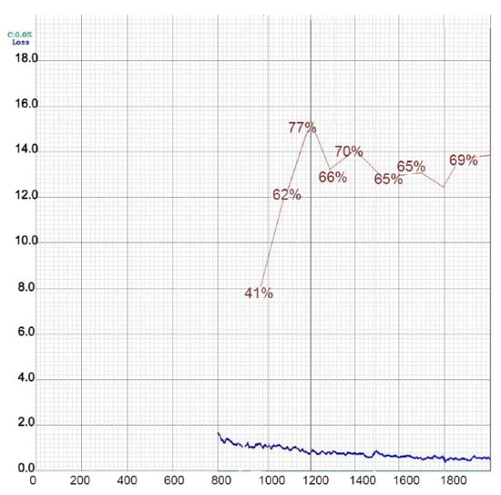
Figure 17.
Loss and mAP performance during the training of YOLOv4 in the first case.
We noticed that the highest mAP was achieved around the 1200th step, after which it fluctuated. However, the model saved the weight periodically at each 1000th step, so for the testing we chose the weight file with the highest mean average precision. The first calculation of the mAP was carried out around the 1000th step. Figure 18 shows the training results for the third version of YOLO in the first (a) and second (b) cases.
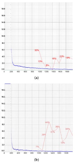
Figure 18.
Representations of loss and mAP values during the training of YOLOv3 in the first (a) and second (b) cases.
The reason for the poor results in mAP and recall was due to the large number of false negative results. During the training of the first case, we recorded 16 false negative detections, while only 7 true positive and 3 false positive detections were recorded in the first case. In the third case, there were no true positive cases, which was why all precision, recall, and F1 score values were calculated to be zero. We could conclude that YOLOv3 performed very badly when there were many negative samples. In order to obtain the bounding box during the testing phase, the threshold was lowered to 0.3 and even to 0.1 in some cases. These low confidence scores are shown in Figure 19. We can see that the confidence score in the first image was only 0.11, in which case the threshold had to be lowered to 0.1, while in the second image, the confidence of prediction was 0.41. These values were significantly lower compared to the other models, which predicted the same objects with confidence scores of up to 0.95.
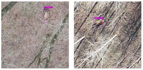
Figure 19.
Illustration of bounding boxes and confidence score predictions of YOLOv3 in the second case, when it achieved the highest mAP.
The performance of the compressed YOLOv4 is shown in Figure 20 and Figure 21 for all three cases. Even though YOLOv4-tiny achieved better precision in the second case, when the negative samples were added, its recall was much higher in the first case, while the precision was only 0.04% lower. In the counting context, recall was more important, as it measured how many of the deer were detected, whereas precision measured how confident one could be that the detected object was actually a deer. In general, the recall was lower than the precision in each case, which suggested that within the detected objects there were more true positive than false positive detections. Given that the training time of this model was very short and the results were as favorable as in YOLOv4, we concluded that this model worked the best for the given problem.
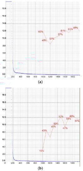
Figure 20.
Representations of loss and mAP values during the training of YOLOv4-tiny in the first two setups, with a different number of training images. In the first case (a), the highest mAP achieved was 65.11%, while in the second case (b) that value was slightly lower at 63.00%. The loss value remained low at all times. (a) Setup 1. (b) Setup 2.
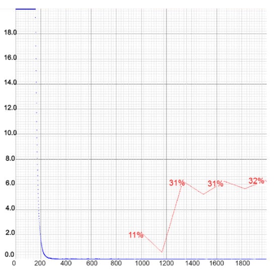
Figure 21.
Representations of loss and mAP values during the training of YOLOv4-tiny in the setup with the highest number of training images. Chart shows poor performance of the model due to the large number of negative samples. The loss value remained low.
The fact that deep CNNs could actually decrease the accuracy in the case of small and medium objects, as all the relevant information disappeared, could explain why YOLOv4-tiny achieved such good results and real-time performance, given its structure. That is, the compressed YOLOv4 comprises only 21 convolutional layers, as opposed to the 110 used in YOLO4 and the 75 layers in YOLOv3. Moreover, except for YOLOv4-tiny, which yielded high confidence scores even for small objects, all the models were less confident when predicting small objects compared to medium objects. From Figure 13 and Figure 14, we can see that the mAP score for medium objects was much higher than for small objects. The same was true for the recall. No large bounding boxes were detected during the training.
Another upside of the compressed YOLOv4 structure was its very fast training speed. The training time of the YOLOv4 model was approximately 8 h when trained on 108 images. This time was doubled in the third case, when the model was trained on 1990 images. On the other hand, the training of YOLOv4-tiny took a maximum of only 2 h for both cases. Therefore, even though YOLOv4 performed slightly better than its compressed version, YOLOv4-tiny had a training speed up to eight times faster; hence, it was better in terms of real-time performance. Taking this into account, the differences in precision and mAP values are negligible if one is in need of fast results.
Moreover, in [30], the authors stated that increasing the image size from the default of 416 × 416 to any larger number that is a multiple of 32 would increase the precision. To extend our research, we conducted an exploratory analysis of the performance of YOLOv4-tiny in several new cases, due to its fast training time. We trained this model using images with input sizes of 512 × 512 and 608 × 608 and confirmed these authors’ statement with our results. The charts of these training processes are shown in Figure 22. Increasing the network resolution to 512 × 512 yielded an mAP value of 68.87%, which was 3.76% higher than the highest value for the 416 × 416 images. The precision also increased from 0.79 to 0.85, which was among the highest precision values obtained in our work. Increasing the resolution even more improved the results as well. The result obtained for mAP was only slightly lower at 68.18%, but all the other measures—precision, recall, and F1 score—were improved, with values of 0.86, 0.60, and 0.71, respectively. After the testing of the model, we were able to obtain the bounding boxes with a confidence score of up to 0.99. In all five cases, the tested loss retained an acceptably low level.
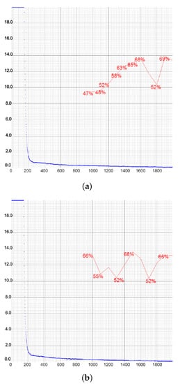
Figure 22.
Charts of the YOLOv4-tiny training with the network resolution increased to 512 × 512 (a) and 608 × 608 (b).
Finally, from Table 5, Table 6 and Table 7, we noticed that all detectors obtained better results for the first and second setups than for the third setup, e.g., with respective mAP values of 72.35% and 50.52% for YOLOv4. This showed that introducing too many negative samples led to a loss in performance in all cases.
5.1. Challenges
Dealing with the detection of small target objects was a challenging task, in which we faced many issues. One of the main problems was the diversity of the input images, as shown in Figure 23. For instance, images could have different resolutions and different sizes, and small objects could be overlapped by other objects. When this happened, the model usually produced a false negative prediction, i.e., not detecting a deer when there was in fact one present.
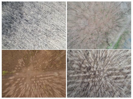
Figure 23.
Example of the image diversity of our dataset. There were huge variations in the background, with illumination differences due to weather, season, and shadows.
Two such examples can be found in Figure 24. Due to the overlap between the UAV images, it might occasionally be possible for one animal to appear in multiple images, producing an error in the final count. Furthermore, if seen from above, animals often tend to be hard to distinguish from various stationary objects such as tree trunks, rocks, and dirt mounds.
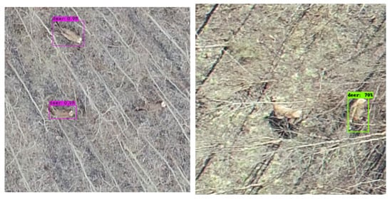
Figure 24.
Illustration of false negative predictions of YOLOv4 (left) and SSD (right) models. We can see that this could happen when the object appeared blurry (as in the left case) or when the animal was overlapped by branches or in motion (as in the right case).
What is more, in images this large, it was often not possible for the naked eye to detect objects of interest, as shown in Figure 25. That is, to achieve a high performance, the images needed to be analyzed at the pixel or small-region level. However, due to the low contrast and cluttered images, it became difficult to identify whether a particular region or pixel based on local information represented an animal or the background. Given that one deer in an image with a size of 4000 × 3000 occupied only up to 500 pixels, and that some images contained only one deer, after the tiling of the image, the extremely small objects appeared much more blurred, since they contained fewer pixels.
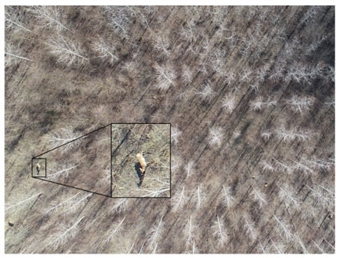
Figure 25.
Example of small target objects in our input images. Given an image this large, it is difficult to locate and recognize the animal, for both humans and machines.
Additional challenge of class imbalance can occur in some models that have background as a class. In general, this problem occurs when some classes appear much more frequent than the others. In the case of this study, where we dealt with only one class, we encountered this problem only with the background class in specific models. Models such as SSD treated the background as class 0, while deer were enumerated as class 1. In this case, using images with sizes of at least 4000 × 3000 pixels, the prominence of the background class was substantially greater. We made a distinction between these two classes during the labeling process. While drawing the bounding boxes, we made a separation between the foreground (the objects) and the background (everything else). The bounding box was then a rough estimation of the foreground and the background, given that it had a rectangular shape. To address the problem of class imbalance, we applied the tiling function described in Section 3.3.
Another problem that we encountered during this work was the small size of the dataset. However, with the development of the state-of-the-art pre-trained models, the need for large datasets has been reduced using different techniques, such as transfer learning. Therefore, by using pre-trained weights, we were able to build a reliable model using a relatively small custom dataset.
6. Conclusions
In this paper, we presented models that work on UAV images and can assist humans in counting and monitoring wild animals. This task is of central importance to many environmental, as well as economic, issues. Four deep learning convolutional networks were trained to recognize and count deer in the Plavna hunting ground, in order to preserve an optimal number at all times. We used pre-trained weights and further trained these models on our own data. The results showed that the CNN managed to yield high-performance predictions, even on images this large. It also demonstrated a high accuracy, comparable to human detection capabilities. The animal detection with the You Only Look Once algorithm achieved a precision of 86%, with an mAP of up to 70.45%. The overall mean average precision of all the models in the optimal setup was in the range of 65–70%, except for YOLOv3, which reached only 0.38%. The highest accuracy, 70.45%, was achieved with the fourth version of YOLO in the second setup, that is, when there was an equal number of positive and negative samples. However, even though the compressed version yielded somewhat lower accuracy, with an mAP of 68.87%, when the network resolution was increased, the training, testing, and counting processes were significantly faster. This model also outperformed the other tested models in the counting process, with 157 out of 169 deer detected. Although the models were trained to recognize only one class, deer, the process is easily extendable to detect and track other types of animals, provided that there are sufficient training data. This study also showcased the feasibility of using UAV imagery in combination with CNNs as a promising wildlife surveying technique. In addition, we showed that it is possible to generalize detection to populations outside of the site of the training data. By utilizing this information, more data from diverse UAV images could be gathered to improve the performance of the models.
Future work will include experiments using this method on other animal databases. Instead of SSD300, an SSD512 model could be trained, as increasing the input size (in this case from 300 × 300 to 512 × 512) could help improve the detection of small objects. Based on the authors’ suggestions, we found that this model worked better on smaller objects than SSD300. Another similar suggestion for future work came from the authors of the YOLO network, who recommended increasing the resolution of the input images to 512 × 512 or 608 × 608, which we tested only for the YOLOv4-tiny model. Our results showed a slight increase in both the precision and mean average precision of YOLOV4-tiny, and we believe the same would apply for YOLOv4. Given that YOLOv4 yielded a higher mAP, future work should include training this model on larger image sizes as well. We also recommend trying the newest version of You Only Look Once (version five), as well as its compressed version, which showed promising results in related works.
Future work will also cover the problem of class imbalance. An initial solution to overcome the imbalance problem might be to artificially balance the dataset by oversampling, i.e., repeating each animal instance to match the total number of background locations. While this has been shown to work well for other tasks, in some cases it can cause the CNN to overfit. The inverse is also a possibility, as well as undersampling, which involves reducing the number of background samples to match the number of other classes. The drawback of this method is that it can reduce the model’s ability to learn the variability of the background, which leads the model to misidentify everything that looks even remotely similar to an animal.
Author Contributions
Conceptualization, B.B., B.T. and O.M.; methodology, O.M., B.P., A.B. and K.R.; software, K.R. and B.P.; formal analysis, M.V. and A.B.; investigation, B.I. and M.V.; resources, B.I. and M.V.; data curation, K.R. and B.I.; writing—original draft preparation, K.R.; writing—review and editing, B.B., O.M., B.I. and B.P.; supervision, O.M. and V.C.; project administration, B.B., V.C. and A.B.; funding acquisition, B.T., B.B. and V.C. All authors have read and agreed to the published version of the manuscript.
Funding
This work is supported through ANTARES project that has received funding from the European Union’s Horizon 2020 research and innovation programme under grant agreement SGA-CSA. No. 739570 under FPA No. 664387—https://doi.org/10.3030/739570. The authors acknowledge financial support from the Ministry of Education, Science and Technological Development of the Republic of Serbia (Grant No. 451-03-68/2022-14/200117 and 451-03-47/2023-01/200358).
Data Availability Statement
Protected by the NDA.
Acknowledgments
The authors wish to thank Vojvodinašume for their generous contribution in organizing the field scanning and providing practical insights into the observed problem.
Conflicts of Interest
No potential conflict of interest is reported by the authors.
Abbreviations
The following abbreviations are used in this manuscript:
| UAV | Unmanned aerial vehicle |
| YOLO | You Only Look Once |
| SSD | Single Shot Multibox Detector |
| CDFD | Context-aware Dense Feature Distillation |
| mAP | Mean average precision |
| CNNs | Convolutional neural networks |
| CDFD | Context-aware Dense Feature Distillation |
| AI | Artificial intelligence |
| FPS | Frames per second |
| NMS | Non-maximum suppression |
| API | Application programming interface |
| ROIs | Regions of interest |
| TP | True positive |
| TN | True negative |
| FP | False positive |
| FN | False negative |
| IOU | Intersection Over Union |
References
- Chamoso, P.; Raveane, W.; Parra, V.; González, A. UAVs applied to the counting and monitoring of animals. In Proceedings of the Ambient Intelligence-software and Applications, Salamanca, Spain, 4–6 June 2014; Springer: Cham, Switzerland, 2014; pp. 71–80. [Google Scholar]
- Prosekov, A.; Kuznetsov, A.; Rada, A.; Ivanova, S. Methods for monitoring large terrestrial animals in the wild. Forests 2020, 11, 808. [Google Scholar] [CrossRef]
- Kellenberger, B.; Marcos, D.; Tuia, D. Detecting mammals in UAV images: Best practices to address a substantially imbalanced dataset with deep learning. Remote Sens. Environ. 2018, 216, 139–153. [Google Scholar] [CrossRef]
- Gemert, J.C.v.; Verschoor, C.R.; Mettes, P.; Epema, K.; Koh, L.P.; Wich, S. Nature conservation drones for automatic localization and counting of animals. In Proceedings of the European Conference on Computer Vision, Zurich, Switzerland, 6–7 September 2014; Springer: Cham, Switzerland, 2014; pp. 255–270. [Google Scholar]
- Darshanraj N, P.K. Animal Counting and Detection Using Convolutional Neural Network. Int. Res. J. Eng. Technol. (IRJET) 2020, 7, 7. [Google Scholar]
- Wang, C.Y.; Bochkovskiy, A.; Liao, H.Y.M. Scaled-YOLOv4: Scaling Cross Stage Partial Network. In Proceedings of the IEEE/CVF Conference on Computer Vision and Pattern Recognition (CVPR), online, 19–25 June 2021; pp. 13029–13038. [Google Scholar]
- Rosli, M.S.A.B.; Isa, I.S.; Maruzuki, M.I.F.; Sulaiman, S.N.; Ahmad, I. Underwater animal detection using YOLOV4. In Proceedings of the 2021 11th IEEE International Conference on Control System, Computing and Engineering (ICCSCE), Penang, Malaysia, 27–28 August 2021; IEEE: New York, NY, USA, 2021; pp. 158–163. [Google Scholar]
- Jiang, Z.; Zhao, L.; Li, S.; Jia, Y. Real-time object detection method based on improved YOLOv4-tiny. arXiv 2020, arXiv:2011.04244. [Google Scholar]
- Schütz, A.K.; Schöler, V.; Krause, E.T.; Fischer, M.; Müller, T.; Freuling, C.M.; Conraths, F.J.; Stanke, M.; Homeier-Bachmann, T.; Lentz, H.H. Application of YOLOv4 for Detection and Motion Monitoring of Red Foxes. Animals 2021, 11, 1723. [Google Scholar] [CrossRef] [PubMed]
- Duporge, I.; Isupova, O.; Reece, S.; Macdonald, D.W.; Wang, T. Using very-high-resolution satellite imagery and deep learning to detect and count African elephants in heterogeneous landscapes. Remote Sens. Ecol. Conserv. 2021, 7, 369–381. [Google Scholar] [CrossRef]
- Gu, L.; Fang, Q.; Wang, Z.; Popov, E.; Dong, G. Learning Lightweight and Superior Detectors with Feature Distillation for Onboard Remote Sensing Object Detection. Remote Sens. 2023, 15, 370. [Google Scholar] [CrossRef]
- Han, L.; Tao, P.; Martin, R.R. Livestock detection in aerial images using a fully convolutional network. Comput. Vis. Media 2019, 5, 221–228. [Google Scholar] [CrossRef]
- Gomez, A.; Diez, G.; Salazar, A.; Diaz, A. Animal identification in low quality camera-trap images using very deep convolutional neural networks and confidence thresholds. In Proceedings of the Advances in Visual Computing: 12th International Symposium, ISVC 2016, Part I, Las Vegas, NV, USA, 12–14 December 2016; Springer: Cham, Switzerland, 2016; pp. 747–756. [Google Scholar]
- Verschoor, C.R. Verschoor Aerial Cow Dataset. 2013. Available online: https://isis-data.science.uva.nl/jvgemert/conservationDronesECCV14w/ (accessed on 29 December 2022).
- Verma, G.K.; Gupta, P. Wild animal detection using deep convolutional neural network. In Proceedings of the 2nd International Conference on Computer Vision & Image Processing, Hong Kong, China, 29–31 December 2018; Springer: Cham, Switzerland, 2018; pp. 327–338. [Google Scholar]
- Hong, T.; Liang, H.; Yang, Q.; Fang, L.; Kadoch, M.; Cheriet, M. A Real-Time Tracking Algorithm for Multi-Target UAV Based on Deep Learning. Remote. Sens. 2022, 15, 2. [Google Scholar] [CrossRef]
- Bochkovskiy, A.; Wang, C.Y.; Liao, H.Y.M. Yolov4: Optimal speed and accuracy of object detection. arXiv 2020, arXiv:2004.10934. [Google Scholar]
- Benali Amjoud, A.; Amrouch, M. Convolutional neural networks backbones for object detection. In Proceedings of the International Conference on Image and Signal Processing, Marrakesh, Morocco, 4–6 June 2020; Springer: Cham, Switzerland, 2020; pp. 282–289. [Google Scholar]
- Redmon, J.; Divvala, S.; Girshick, R.; Farhadi, A. You only look once: Unified, real-time object detection. In Proceedings of the IEEE Conference on Computer Vision and Pattern Recognition, Las Vegas, NV, USA, 26 June–1 July 2016; pp. 779–788. [Google Scholar]
- Yun, S.; Han, D.; Oh, S.J.; Chun, S.; Choe, J.; Yoo, Y. Cutmix: Regularization strategy to train strong classifiers with localizable features. In Proceedings of the IEEE/CVF International Conference on Computer Vision, Seoul, Republic of Korea, 27 October–2 November 2019; pp. 6023–6032. [Google Scholar]
- Liu, W.; Anguelov, D.; Erhan, D.; Szegedy, C.; Reed, S.; Fu, C.Y.; Berg, A.C. Ssd: Single shot multibox detector. In Proceedings of the European Conference on Computer Vision, Amsterdam, The Netherlands, 11–14 October 2016; Springer: Cham, Switzerland, 2016; pp. 21–37. [Google Scholar]
- Huang, J.; Rathod, V.; Sun, C.; Zhu, M.; Korattikara, A.; Fathi, A.; Fischer, I.; Wojna, Z.; Song, Y.; Guadarrama, S.; et al. Speed/accuracy trade-offs for modern convolutional object detectors. In Proceedings of the IEEE Conference on Computer Vision and Pattern Recognition, Honolulu, HI, USA, 21–26 July 2017; pp. 7310–7311. [Google Scholar]
- Lin, T.Y.; Maire, M.; Belongie, S.; Hays, J.; Perona, P.; Ramanan, D.; Dollár, P.; Zitnick, C.L. Microsoft coco: Common objects in context. In Proceedings of the European Conference on Computer Vision, Zurich, Switzerland, 6–12 September 2014; Springer: Cham, Switzerland, 2014; pp. 740–755. [Google Scholar]
- Everingham, M.; Van Gool, L.; Williams, C.K.I.; Winn, J.; Zisserman, A. The Pascal Visual Object Classes (VOC) Challenge. Int. J. Comput. Vis. 2010, 88, 303–338. [Google Scholar] [CrossRef]
- Tzutalin, L. Git Code. 2015. Available online: https://github.com/tzutalin/labelImg (accessed on 29 December 2022).
- Wang, C.Y.; Liao, H.Y.M.; Wu, Y.H.; Chen, P.Y.; Hsieh, J.W.; Yeh, I.H. CSPNet: A new backbone that can enhance learning capability of CNN. In Proceedings of the IEEE/CVF Conference on Computer Vision and Pattern Recognition Workshops, Seattle, WA, USA, 14–19 June 2020; pp. 390–391. [Google Scholar]
- He, K.; Zhang, X.; Ren, S.; Sun, J. Spatial pyramid pooling in deep convolutional networks for visual recognition. IEEE Trans. Pattern Anal. Mach. Intell. 2015, 37, 1904–1916. [Google Scholar] [CrossRef] [PubMed]
- Liu, S.; Qi, L.; Qin, H.; Shi, J.; Jia, J. Path aggregation network for instance segmentation. In Proceedings of the IEEE Conference on Computer Vision and Pattern Recognition, Salt Lake City, UT, USA, 18–23 June 2018; pp. 8759–8768. [Google Scholar]
- Deng, J.; Dong, W.; Socher, R.; Li, L.J.; Li, K.; Fei-Fei, L. Imagenet: A large-scale hierarchical image database. In Proceedings of the 2009 IEEE Conference on Computer Vision and Pattern Recognition, Miami, FL, USA, 20–25 June 2009; IEEE: New York, NY, USA, 2019; pp. 248–255. [Google Scholar]
- Bochkovskiy, A. Darknet Repository. Available online: https://sourcegraph.com/github.com/AlexeyAB/darknet (accessed on 29 December 2022).
- Padilla, R.; Passos, W.L.; Dias, T.L.; Netto, S.L.; da Silva, E.A. A comparative analysis of object detection metrics with a companion open-source toolkit. Electronics 2021, 10, 279. [Google Scholar] [CrossRef]


Disclaimer/Publisher’s Note: The statements, opinions and data contained in all publications are solely those of the individual author(s) and contributor(s) and not of MDPI and/or the editor(s). MDPI and/or the editor(s) disclaim responsibility for any injury to people or property resulting from any ideas, methods, instructions or products referred to in the content. |
© 2023 by the authors. Licensee MDPI, Basel, Switzerland. This article is an open access article distributed under the terms and conditions of the Creative Commons Attribution (CC BY) license (https://creativecommons.org/licenses/by/4.0/).