Unknown Input Observer-Based Fixed-Time Trajectory Tracking Control for QUAV with Actuator Saturation and Faults

Abstract

The trajectory tracking control problem of a quadrotor unmanned aerial vehicle (QUAV) subject to external disturbances, inertia uncertainties, actuator faults, and input saturation is addressed in this paper. In contrast with previous works, input saturation herein refers to rotor speed saturation rather than thrust and torque saturation. First, the control system is decoupled into translational and rotational subsystems. Then, for both subsystems, two novel fixed-time unknown input observers (UIO) based on disturbance filtering are developed to estimate the lumped disturbance rapidly and precisely without awareness of the boundary of disturbances. Furthermore, fixed-time tracking controllers for translational and rotational subsystems are proposed based on the estimation values provided by UIO to stabilize tracking errors into a small region in fixed time regardless of the initial values. The theoretical analysis based on the Lyapunov method is presented to demonstrate the stability. Finally, the simulation results show that the proposed control method is effective. The comparison simulation is carried out to validate superiority of the proposed observer and its advantage can be summed up as: (1) the upper bound of the disturbance or its derivative is not needed; (2) the estimation results are smoother and the observation precision is higher due to the absence of sign function; (3) the mutant disturbance can be also estimated quickly and precisely.

1. Introduction

In recent years, research on quadrotor unmanned aerial vehicles (QUAVs) has been widely conducted. The interest is sparked by the broad range of tasks for which it can be applied, including aerial photography, inspection monitoring, and agricultural plant protection, all while enjoying the benefits of small size, compact structure, and flexible maneuverability [1,2,3]. However, the QUAV is a multivariable, strongly coupled, nonlinear under-actuated system with four inputs but six degrees of freedom, which makes the control design and stability analysis more complicated [4,5]. As a result, trajectory tracking control of QUAV has become a complicated matter that has been extensively studied.

Traditional linear control strategies, such as PID [6] and LQR [7], are only applicable to linearization models, and control performance for nonlinear systems is hard to guarantee. As a result, numerous nonlinear control schemes, including but not limited to feedback linearization control [8], backstepping control [9,10], and sliding mode control (SMC) [11,12,13], have been developed for the QUAV in order to mitigate the influence of nonlinear characteristics. Moreover, the speed of convergence is regarded as an important parameter for the QUAV’s control systems. Therefore, control systems based on finite-time control have gained significant attention [2,14,15,16,17]. For example, in [14], the authors proposed a fast terminal sliding mode controller (FTSMC) to achieve trajectory tracking control of the QUAV, and the tracking error for desired altitude and attitude was guaranteed to converge to zero in finite time. A finite-time nonlinear disturbance observer (NDO) was also presented to estimate external disturbance acting on altitude and attitude channels of the QUAV. An adaptive command-filtered backstepping sliding mode control scheme was proposed to achieve finite-time tracking control of the QUAV system under modeling uncertainties and external disturbances in [16]. However, the convergence time of finite-time control depends on the initial values of the system. Consequently, fixed-time control is proposed by researchers, and the error can converge to zero in fixed time independent of initial values. Xia and Son [18] addressed the fixed-time control problem of autonomous ship landing operations of vertical take-off and landing UAVs subject to external disturbances. An anti-saturation adaptive fault-tolerant control scheme with fixed-time prescribed performance for the longitudinal model of fixed wing UAV under actuator faults, control input saturation, angle of attack asymmetric constraint, and uncertainties was presented in [19]. Ref. [20] proposed a fixed-time adaptive fast super-twisting disturbance observer to estimate the unknown external disturbance, and a fixed-time controller was designed using a universal barrier Lyapunov function to satisfy asymmetric tracking error constraints.

The external disturbances, inertia uncertainties, and actuator faults often need to be considered in the trajectory tracking control for QUAV [4,11,12,16]. The most efficient strategy for dealing with external disturbances, inertia uncertainties, and actuator faults is to compensate for their negative impacts on the system via exact estimation. As a result, numerous disturbance observer-based control approaches, such as those based on the extended state observer (ESO) [21,22], the super-twisting disturbance observer (STDO) [20,23,24], and the sliding mode disturbance observer (SMDO) [25,26], have been developed. Nonetheless, the observers mentioned above all require that disturbance is continuously differentiable and its derivative is bounded or known beforehand. When the disturbance changes suddenly, its derivative is infinite, hence the observation performance cannot be guaranteed in this case. Moreover, the sign function is adopted in ESO and SMDO, so the estimation of disturbance may be not smooth. To overcome this constraint, by introducing a reference auxiliary system, a nonlinear observer was developed to accomplish a high-accuracy estimation for the lumped disturbance in fixed time without being aware of the boundary of disturbances in [27]. However, the design process of this observer is complicated. The control problem of nonlinear robotic systems suffering from actuator failure was investigated in [28]. Based on the state transformation, a finite-time unknown input observer (UIO) was designed to estimate the lumped unknown input. Nevertheless, the observer in [28] can only estimate the lumped unknown input in finite time.

Furthermore, the output capability of the actuator is often limited; hence, input saturation should be frequently considered in trajectory tracking control. In [29], the finite-time trajectory tracking problem for a novel 12-rotor UAV with input saturation was investigated. The authors of [30] addressed the finite-time tracking control problem of the QUAV subject to external disturbances, parametric uncertainties, actuator faults, and input saturation. Cao and Lynch [31] studied the position control of a QUAV with state and input constraints using an inner-outer loop control structure. However, all the works of literature cited above simply supply the saturation values of the control force and torque, which is inexhaustive. The control input signals of the QUAV are determined by the rotor speed of the four motors, and the rotor speed of each motor is different and has an upper limit. In fact, as long as one motor’s rotor speed is saturated, the control input signals related to that motor’s rotor speed are constrained. Therefore, rotor speed saturation is considered in this paper.

Motivated by the preceding discussions, this work focuses on developing a fixed-time control method for the QUAV trajectory tracking control when external disturbances, inertia uncertainties, actuator faults, and input saturation are considered. In comparison to the current investigation results, the major contributions of this work can be summarized as follows:

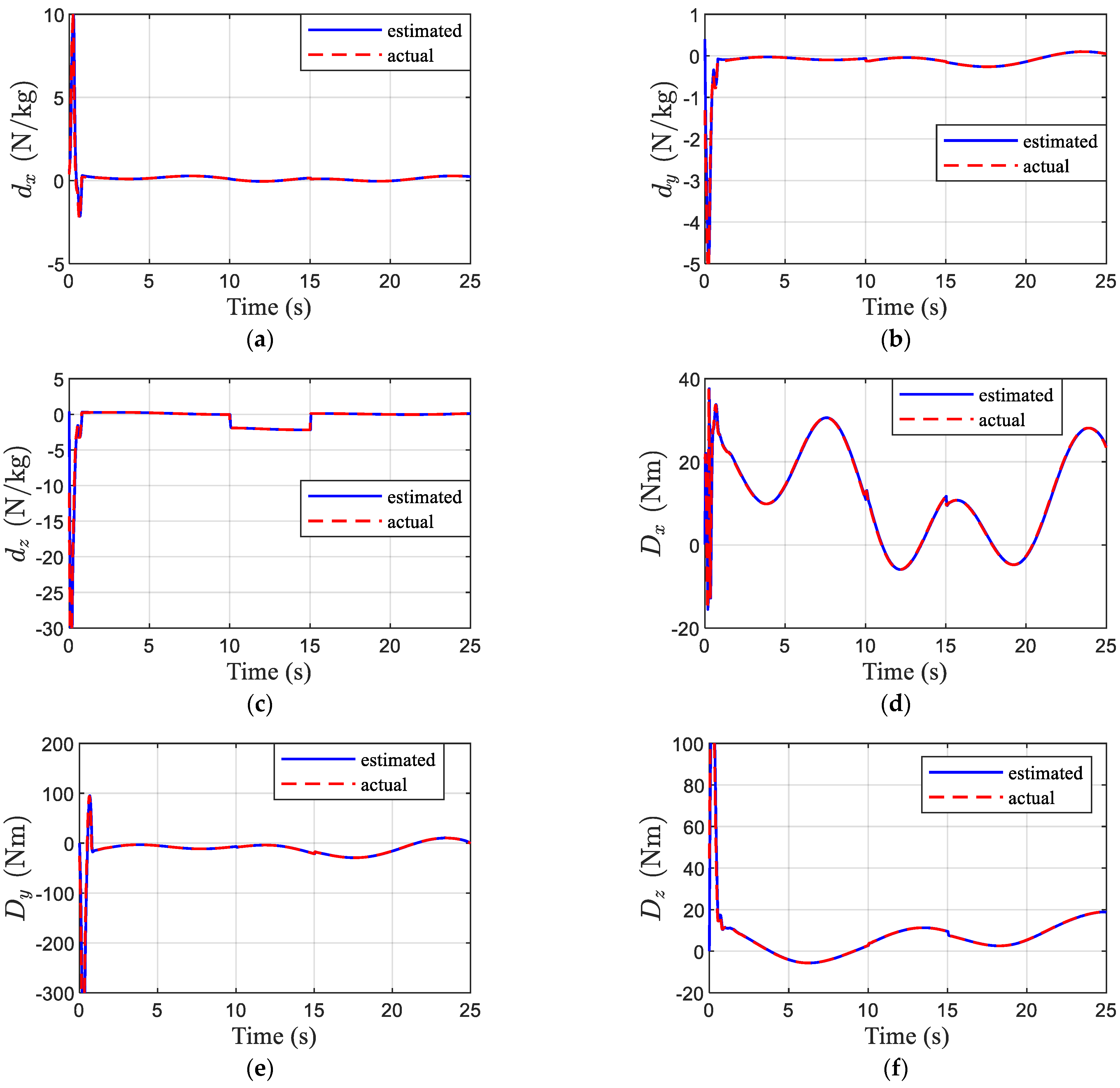
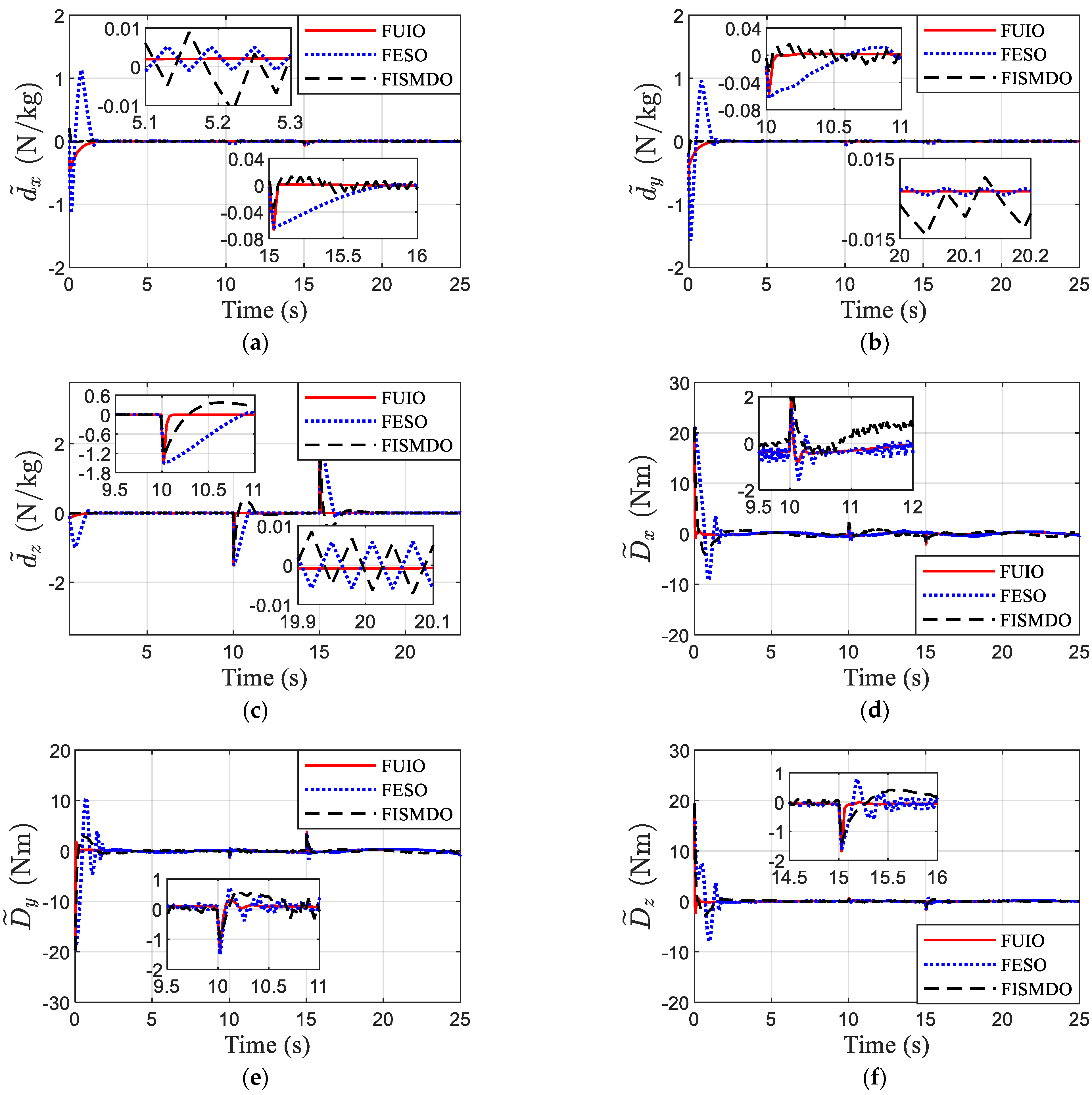
• The fixed-time UIOs are designed to estimate the lumped disturbance for translational and rotational subsystems, with the estimation error able to converge to zero in fixed time. The proposed observer has three advantages and can overcome the limitations described in [20,21,22,23,24,25,26]. Firstly, it does not require prior knowledge of the upper bound of disturbance or its derivative. Additionally, the sign function is absent in UIO, which implies that the observation of disturbance is smoother and the estimation precision is higher. Furthermore, it can estimate the mutant disturbance accurately and rapidly.
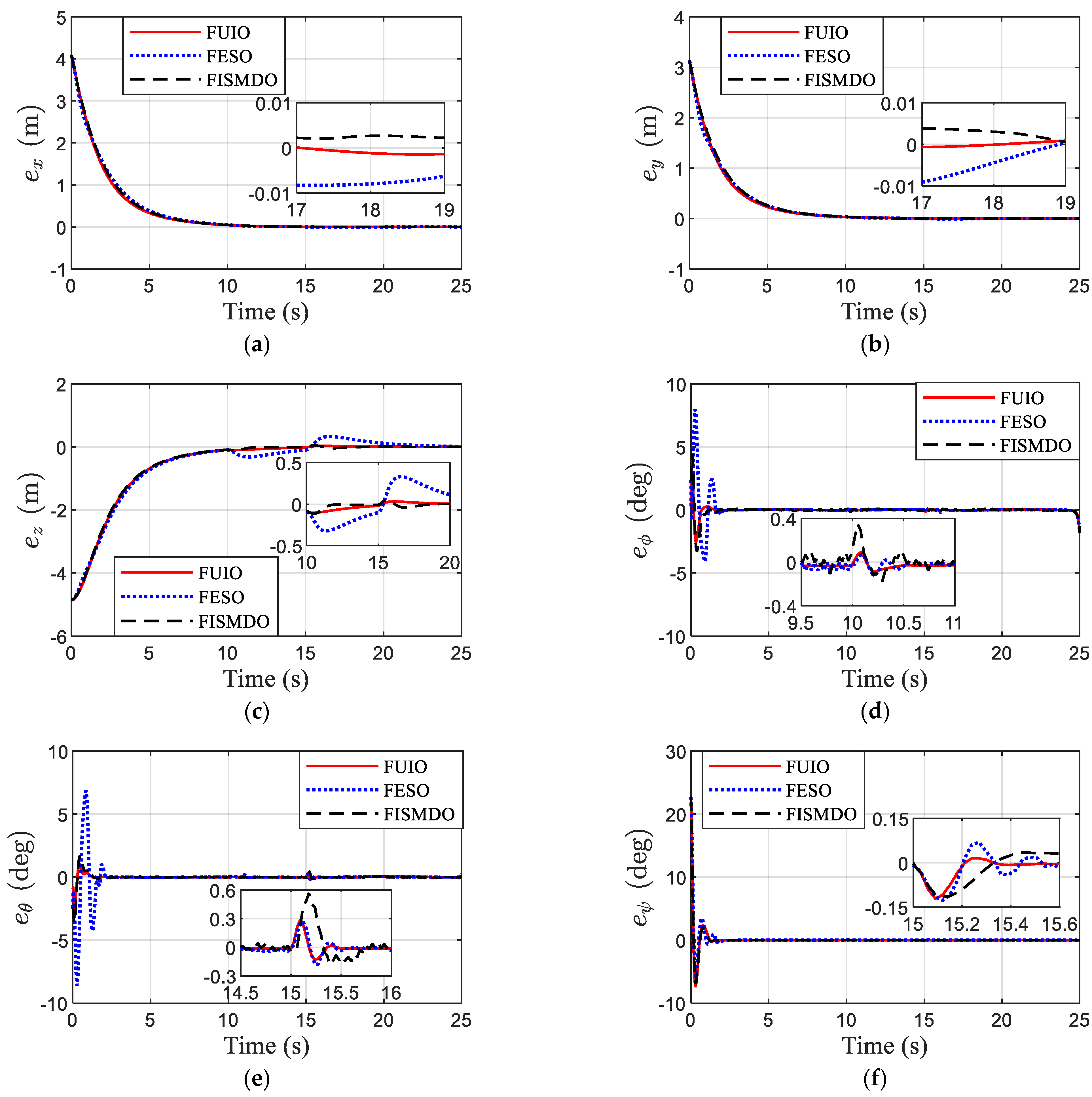
• Based on the estimation values provided by fixed-time UIO, fixed-time tracking controllers are proposed for both subsystems to stabilize the tracking error into a small region in fixed time. In contrast with the existing controllers with finite-time stability [2,14,15,16,17], the proposed fixed-time controllers’ convergence time is independent of initial values.
• External disturbances, inertia uncertainties, actuator faults, and input saturation are all considered in this paper. In [4,11,12,16,28], input saturation is not considered. Although input saturation is considered in [29,30,31], they simply give the saturation values of control input signals. In this paper, input saturation is constraining the rotor speed rather than the control input signals, which is more reasonable.

The rest of this paper can be summarized as follows. In Section 2, the model of the QUAV, the control objectives, and some useful lemmas are given. The control schemes for translational and rotational subsystems are proposed in Section 3. The simulation results show the effectiveness of the proposed control methods in Section 4. Finally, the conclusions are drawn in Section 5.

2. Mathematical Model and Problem Formulation

In this section, the mathematical model of QUAV is established first. Then, for the convenience of controller design, the model is simplified. Some useful lemmas are also provided.

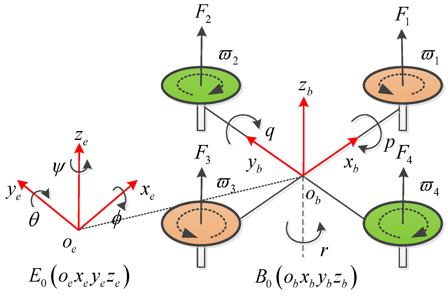
2.1. Mathematical Model of QUAV

The QUAV framework with a symmetrical structure is investigated as illustrated in Figure 1. The flight motions can be subdivided into translational motion and rotational motion. To describe the kinematics and dynamics of QUAV, the earth-fixed frame $E_0:o_e{x}_e{y}_e{z}_e$ and the body-fixed frame $B_0:o_b{x}_b{y}_b{z}_b$ are defined as shown in Figure 1. For the translational motion, $p=[x,y,z{]}^{\mathrm{T}}$ with respect to $E_0$ and $v=[u,v,w{]}^{\mathrm{T}}$ with respect to $B_0$ stand for the position and the velocity of the QUAV, respectively. For the rotational motion, $\Theta =[\varphi ,\theta ,\psi {]}^{\mathrm{T}}$ in $E_0$ and $\omega =[p,q,r{]}^{\mathrm{T}}$ in $B_0$ represent the Euler angle and the angular velocity of the QUAV, respectively, where the three channels represent roll, pitch, and yaw channels in sequence.

Based on the previous descriptions and the Newton–Euler equation, the mathematical model of translational and rotational motion can be expressed as

$$\{\begin{array}{l}\dot{p}=v\\ \dot{v}=-g{e}_z+\frac{T}{m}R{e}_z+{\Delta }_1\end{array}$$

(1)

$$\{\begin{array}{c}\dot{\Theta }=W\omega \hfill \\ \mathbf{J}\dot{\mathbf{\omega }}=-{\mathbf{\omega }}^{\times }\mathbf{J}\mathbf{\omega }+\tau +{\Delta }_2\hfill \end{array}$$

(2)

where $g$ is the gravitational acceleration and $e_z={[0,0,1]}^{\mathrm{T}}$, $m$ is the total mass, ${\Delta }_1$ and ${\Delta }_2$ are external disturbances, $T$ and $\tau$ are the total thrust and attitude control torque vector, respectively. $J=J_0+\Delta J$ denotes the inertia matrix, $J_0$ is the nominal part of the inertia matrix and $\Delta J$ is the uncertainty part. From [32], the inverse of the inertia matrix $J$ can be expressed as

$$\begin{array}{c}{J}^{-1}={(J_0+\Delta J)}^{-1}={(J_0)}^{-1}-{(J_0+J_0\Delta J^{-1}{J}_0)}^{-1}\hfill \\ \hspace{1em}\hspace{1em}=J_0^{-1}+\Delta \tilde{J}\hfill \end{array}$$

(3)

$R$ is the rotation matrix from body-fixed frame to earth-fixed frame

$$R=\left[\begin{array}{ccc}{C}_{\theta }{C}_{\psi }& C_{\psi }{S}_{\theta }{S}_{\varphi }-S_{\psi }{C}_{\varphi }& C_{\psi }{S}_{\theta }{C}_{\varphi }+S_{\psi }{S}_{\varphi }\\ C_{\theta }{S}_{\psi }& S_{\psi }{S}_{\theta }{S}_{\varphi }+C_{\psi }{C}_{\varphi }& S_{\psi }{S}_{\theta }{C}_{\varphi }-C_{\psi }{S}_{\varphi }\\ -S_{\theta }& C_{\theta }{S}_{\varphi }& C_{\theta }{C}_{\varphi }\end{array}\right]$$

(4)

where $S$ represents $\sin (\cdot )$ and $C$ denotes $\cos (\cdot )$. The skew-symmetric matrix ${\omega }^{\times }$ and matrix $W$ are

$${\omega }^{\times }=\left[\begin{array}{ccc}0& -r& q\\ r& 0& -p\\ -q& p& 0\end{array}\right]$$

(5)

$$W=\left[\begin{array}{ccc}1& \tan \theta \sin \varphi & \tan \theta \cos \varphi \\ 0& \cos \varphi & -\sin \varphi \\ 0& \sin \varphi /\cos \theta & \cos \varphi /\cos \theta \end{array}\right]$$

(6)

2.2. Problem Formulation

The mathematical model of translational and rotational subsystems with external disturbances is presented in Equations (1) and (2). Moreover, inertia uncertainties, actuator faults, and input saturation are also considered in this paper.

Considering uncertainties of inertia matrix, $M$ denotes the derivative of the Euler angle, then the mathematical model of rotational subsystem can be arranged as

$$\{\begin{array}{c}\dot{\Theta }={\rm M}\hfill \\ \dot{\mathbf{M}}=W{\mathbf{J}}_0^{-1}\tau +f\hfill \end{array}$$

(7)

where $f=\dot{W}\omega +W{\mathbf{J}}^{-1}\left(-{\mathbf{\omega }}^{\times }\mathbf{J}\mathbf{\omega }+{\Delta }_2\right)+\mathbf{W}\mathbf{\Delta }\tilde{\mathbf{J}}\tau$.

The total thrust and attitude control torque are determined by the combination of four rotors’ speed. The relationship between the total thrust $T$ and attitude control torque $\tau ={[\begin{array}{ccc}{\tau }_x& {\tau }_y& {\tau }_z\end{array}]}^{\mathrm{T}}$ with the rotor speed can be obtained as

$$T=c_1{\mathsf{\nu }}_{\varpi }=\left[\begin{array}{cccc}{c}_T& c_T& c_T& c_T\end{array}\right]{\left[\begin{array}{cccc}{\varpi }_1^2& {\varpi }_2^2& {\varpi }_3^2& {\varpi }_4^2\end{array}\right]}^{\mathrm{T}}$$

(8)

$$\tau =c_2{\mathsf{\nu }}_{\varpi }=\left[\begin{array}{cccc}0& -d{c}_T& 0& d{c}_T\\ -d{c}_T& 0& d{c}_T& 0\\ -c_M& c_M& -c_M& c_M\end{array}\right]\left[\begin{array}{c}{\varpi }_1^2\\ {\varpi }_2^2\\ {\varpi }_3^2\\ {\varpi }_4^2\end{array}\right]$$

(9)

where $c_T$ and $c_M$ are constants, $d$ denotes the distance from rotor endpoint to QUAV center of gravity, and ${\varpi }_i$ is the rotor speed, $i=1,2,3,4$.

The actuators of QUAV are four motors, and the multiplicative fault for actuators is considered here. The actuator faults can be described as

$${\varpi }_{di}={\rho }_i{\varpi }_{ci}\hspace{1em}\hspace{1em}i=1,2,3,4$$

(10)

where ${\rho }_i\in [0,1]$, ${\varpi }_{ci}$ represents the commanded rotor speed by controller and ${\varpi }_{di}$ is the desired rotor speed. Then, the total thrust and attitude control torque can be rewritten as

$$T_d=c_1{\mathsf{\nu }}_{\varpi d}=c_1\mathsf{\rho }{\mathsf{\nu }}_{\varpi c}$$

(11)

$${\tau }_d=c_2{\mathsf{\nu }}_{\varpi d}=c_2\mathsf{\rho }{\mathsf{\nu }}_{\varpi c}$$

(12)

where $\mathsf{\rho }=\mathrm{diag}({\rho }_1^2,{\rho }_2^2,{\rho }_3^2,{\rho }_4^2)$ stands for the health condition of actuators, ${\mathsf{\nu }}_{\varpi d}={[{\varpi }_{d1}^2,{\varpi }_{d2}^2,{\varpi }_{d3}^2,{\varpi }_{d4}^2]}^{\mathrm{T}}$, ${\mathsf{\nu }}_{\varpi c}={[{\varpi }_{c1}^2,{\varpi }_{c2}^2,{\varpi }_{c3}^2,{\varpi }_{c4}^2]}^{\mathrm{T}}$, $T_d$, and ${\mathsf{\tau }}_d$ are the desired total thrust and attitude control torque, respectively.

However, the actual total thrust and attitude control torque may not reach the desired value due to the upper limit of rotor speed. Therefore, input saturation is considered in this paper. Let ${\varpi }_{\max i}$ denote the saturation limit of ${\varpi }_i$. The ${\varpi }_i$ is limited in the following form

$${\varpi }_i=\{\begin{array}{l}{\varpi }_{di}\hspace{0.17em},\hspace{1em}\hspace{1em}{\varpi }_{di}\le {\varpi }_{\max i}\\ {\varpi }_{\max i}\hspace{0.17em},\hspace{1em}\hspace{0.17em}{\varpi }_{di}>{\varpi }_{\max i}\end{array}\hspace{1em}\hspace{1em}i=1,2,3,4$$

(13)

where ${\varpi }_{\max i}$ is a constant normally. However, when actuator faults occur, the saturation limit of rotor speed will also be influenced. Therefore, the saturation limit is different based on whether it occurs with actuator faults or without actuator faults in this paper.

Combining Equations (10) and (13), the relationship between the actual rotor speed ${\varpi }_i$ and the commanded rotor speed by controller ${\varpi }_{ci}$ can be obtained as

$${\varpi }_i=\{\begin{array}{l}{\rho }_i{\varpi }_{ci}\hspace{0.17em},\hspace{1em}\hspace{0.17em}{\rho }_i{\varpi }_{ci}\le {\varpi }_{\max i}\\ {\varpi }_{\max i}\hspace{0.17em},\hspace{1em}\hspace{0.17em}{\rho }_i{\varpi }_{ci}>{\varpi }_{\max i}\end{array}\hspace{1em}\hspace{1em}i=1,2,3,4$$

(14)

For the translational subsystem, we define the virtual control vector as $u={[u_x,u_y,u_z]}^{\mathrm{T}}=-g{e}_z+\frac{T}{m}R{e}_z$. According to Equation (8), the virtual control vector can be expressed as

$$\begin{array}{c}u=-g{e}_z+\frac{T}{m}R{e}_z=-g{e}_z+\frac{1}{m}{c}_1{\mathsf{\nu }}_{\varpi }R{e}_z\hfill \\ \hspace{1em}=-g{e}_z+\frac{1}{m}{c}_1{\mathsf{\nu }}_{\varpi c}R{e}_z+\frac{1}{m}{c}_1\left({\mathsf{\nu }}_{\varpi }-{\mathsf{\nu }}_{\varpi c}\right)R{e}_z\hfill \\ \hspace{1em}=-g{e}_z+\frac{T_c}{m}R{e}_z+\frac{1}{m}{c}_1\left({\mathsf{\nu }}_{\varpi }-{\mathsf{\nu }}_{\varpi c}\right)R{e}_z\hfill \\ \hspace{1em}=u_c+\frac{1}{m}{c}_1\left({\mathsf{\nu }}_{\varpi }-{\mathsf{\nu }}_{\varpi c}\right)R{e}_z\hfill \end{array}$$

(15)

where $T_c=c_1{\mathsf{\nu }}_{\varpi c}$ denotes the commanded total thrust by controller. Then, we can obtain a simplified mathematical model

$$\{\begin{array}{l}\dot{p}=v\\ \dot{v}=u_c+d\end{array}$$

(16)

where $u_c={[u_{cx},u_{cy},u_{cz}]}^{\mathrm{T}}$ is the controller to be designed for the translational subsystem, and $d={[d_x,d_y,d_z]}^{\mathrm{T}}$ is the lumped disturbance containing external disturbances, actuator faults, and input saturation and can be expressed as

$$d=\frac{1}{m}{c}_1\left({\mathsf{\nu }}_{\varpi }-{\mathsf{\nu }}_{\varpi c}\right)R{e}_z+{\Delta }_1$$

(17)

According to Equation (9), we can obtain

$$\begin{array}{c}\tau =c_2{\mathsf{\nu }}_{\varpi }=c_2{\mathsf{\nu }}_{\varpi c}+c_2\left({\mathsf{\nu }}_{\varpi }-{\mathsf{\nu }}_{\varpi c}\right)\\ \hspace{0.17em}\hspace{0.17em}\hspace{1em}\hspace{0.17em}\hspace{0.17em}\hspace{0.17em}={\tau }_c+c_2\left({\mathsf{\nu }}_{\varpi }-{\mathsf{\nu }}_{\varpi c}\right)\end{array}$$

(18)

where ${\tau }_c={[{\tau }_{cx},{\tau }_{cy},{\tau }_{cz}]}^{\mathrm{T}}=c_2{\mathsf{\nu }}_{\varpi c}$ represents the attitude control torque to be designed. Substituting Equation (18) into Equation (7), the mathematical model of the rotational subsystem can be rewritten as

$$\{\begin{array}{c}\dot{\mathsf{\Theta }}=\mathbf{M}\hfill \\ \dot{\mathbf{M}}=\mathbf{W}{\mathbf{J}}_0^{-1}{\mathsf{\tau }}_c+D\hfill \end{array}$$

(19)

where $D={[D_x,D_y,D_z]}^{\mathrm{T}}$ is the lumped disturbance of the rotational subsystem containing external disturbances, inertia uncertainties, actuator faults, and input saturation and can be expressed as

$$D=\mathbf{W}{\mathbf{J}}_0^{-1}{c}_2\left({\mathsf{\nu }}_{\varpi }-{\mathsf{\nu }}_{\varpi c}\right)+f$$

(20)

The control objective of this work is to design fixed-time UIOs to estimate the lumped disturbance $d$ and $D$ quickly and accurately without awareness of the boundary of disturbances or the derivatives. Then, the fixed-time tracking controllers $u_c$ and ${\mathsf{\tau }}_c$ are designed to stabilize tracking error to zero in fixed time regardless of initial values.

2.3. Notation and Preliminaries

Consider the nonlinear dynamical system

$$\dot{x}=f(x)\hspace{0.17em},x(0)=x_0$$

(21)

where $x={[x_1,x_2,\cdots ,x_n]}^{\mathrm{T}}\in R^n$ is the state vector and $f(x)$ is the nonlinear function.

Definition 1

[33]. The origin of system (21) is globally fixed time stable if it is globally uniformly finite time stable and the settling time function $T$ is globally bounded. There exists a finite constant $T_{\max }\subset R_{+}$ such that $T\le T_{\max }$ and $x(t)=0$ for $t\ge T$ and $x_0\in R^n$. Let $r={[r_1,\cdots ,r_n]}^{\mathrm{T}}\in R^n$, $r_i>0$ be the weight vector. For any $\lambda >0$, $x\in R^n$, and the dilation mapping can be defined as ${\Lambda }_r(x)={[{\lambda }^{r_1}{x}_1,{\lambda }^{r_2}{x}_2,\cdots ,{\lambda }^{r_n}{x}_n]}^{\mathrm{T}}\in R^n$.

Definition 2

[34]. A vector field $f(x)\in R^n$ is said to be homogeneous with degree $k$ with respect to weight vector $r={[r_1,\cdots ,r_n]}^{\mathrm{T}}\in R^n$ if we have $f_i({\Lambda }_r(x))={\lambda }^{k+r_i}{f}_i(x)$ for any $\lambda >0$,$x\in R^n$.

Definition 3

[34]. A vector field $f(x)\in R^n$ is said to be homogeneous in the 0-limit with triple $(r_0,k_0,f_0(x))$, where $r_0\in R^n$ is the weight vector, $k_0$ is the homogeneous degree, and $f_0(x)$ is the approximating function for $\underset{\lambda \to 0}{\lim }\underset{x\in R^n\backslash 0}{\max }\Vert {\lambda }^{-k_0}{\Lambda }_{r_0}^{-1}f({\Lambda }_{r_0}(x))-f_0(x)\Vert =0$.

Definition 4

[34]. A vector field $f(x)\in R^n$ is said to be homogeneous in the $\infty$-limit with triple $(r_{\infty },k_{\infty },f_{\infty }(x))$, where $r_{\infty }\in R^n$ is the weight vector, $k_{\infty }$ is the homogeneous degree, and $f_{\infty }(x)$ is the approximating function for $\underset{\lambda \to \infty }{\lim }\underset{x\in R^n\backslash 0}{\max }\Vert {\lambda }^{-k_{\infty }}{\Lambda }_{r_{\infty }}^{-1}f({\Lambda }_{r_{\infty }}(x))-f_{\infty }(x)\Vert =0$.

Definition 5

[35]. A vector field $f(x)\in R^n$ is said to be homogeneous in the bi-limit if it is homogeneous in the 0-limit and $\infty$-limit simultaneously.

Lemma 1

[35]. For nonlinear system (21), we suppose the vector field  $f(x)\in R^n$ is homogeneous in the 0-limit and $\infty$-limit simultaneously with triples $(r_0,k_0,f_0(x))$ and $(r_{\infty },k_{\infty },f_{\infty }(x))$. If the origin of system $\dot{x}=f(x)$, $\dot{x}=f_0(x)$, $\dot{x}=f_{\infty }(x)$ is globally asymptotically stable, then the origin of (21) is fixed time stable when $k_{\infty }>0>k_0$ holds.

Lemma 2

[33]. Suppose $\Psi =R^n$ and there exists a Lyapunov function $V\left(x\left(t\right)\right)$ that satisfies $\dot{V}\left(x\left(t\right)\right)\le -\left(l_1{V}^{{\vartheta }_1}\left(x\left(t\right)\right)+l_2{V}^{{\vartheta }_2}\left(x\left(t\right)\right)\right)$. Parameters $l_1,l_2>0,0<{\vartheta }_1<1$ and ${\vartheta }_2>1$ are positive constants, then the origin of system (21) is fixed time stable and $T\left(x\left(0\right)\right)\le 1/\left[l_1\left(1-{\vartheta }_1\right)\right]+1/\left[l_2\left({\vartheta }_2-1\right)\right]$ for any given initial conditions $x\left(0\right)\in R^n$.

Notation 1.

$\Vert x\Vert =\sqrt{x^{\mathrm{T}}x}$denotes the Euclidean norm, where $x={[x_1,x_2,\cdots ,x_n]}^{\mathrm{T}}\in R^n$. 2) For any $x={[x_1,x_2,\cdots ,x_n]}^{\mathrm{T}}\in R^n$, $sign(x)=x/\Vert x\Vert$, $si{g}^p(x)={\Vert x\Vert }^p•sign(x)$, $\mathrm{sgn}\left(x\right)={\left[sign(x_1),\cdots ,sign(x_n)\right]}^{\mathrm{T}}$, ${\lceil x\rfloor }^a={\left[{\left|x_1\right|}^{a}sign(x_1),\cdots ,{\left|x_n\right|}^{a}sign(x_n)\right]}^{\mathrm{T}}$.

3. Control Scheme

The control block diagram of the proposed control method is presented in Figure 2. The translational subsystem is used to achieve position control with the goal reference $p_d={[x_d,y_d,z_d]}^{\mathrm{T}}$. The rotational subsystem is used to realize attitude control with the command ${\Theta }_d={[{\varphi }_d,{\theta }_d,{\psi }_d]}^{\mathrm{T}}$, which is specifically generated via the attitude command generator. The attitude command generator can be obtained as

$$\{\begin{array}{l}{\varphi }_d=\arcsin \left(\frac{u_{cx}\sin {\psi }_d-u_{cy}\cos {\psi }_d}{\sqrt{u_{cx}^2+u_{cy}^2+{\left(u_{cz}+g\right)}^2}}\right)\\ {\theta }_d=\arctan \left(\frac{u_{cx}\cos {\psi }_d+u_{cy}\sin {\psi }_d}{u_{cz}+g}\right)\end{array}$$

(22)

$$T_c=m\left(\begin{array}{c}{u}_{cx}\left(\sin \theta \cos \psi \cos \varphi +\sin \psi \sin \varphi \right)\hfill \\ +u_{cy}\left(\sin \theta \sin \psi \cos \varphi -\cos \psi \sin \varphi \right)\hfill \\ +\left(u_{cz}+g\right)\cos \theta \cos \varphi \hfill \end{array}\right)$$

(23)

Remark 1.

Unlike the previous articles, the desired command$x_d,y_d,z_d,{\psi }_d$comes from a real trajectory, which considers various constraints. The pseudospectral method is used to generate a discrete trajectory, and then the time-continuous trajectory, which is the reference trajectory in this paper, can be obtained by polynomial curve fitting.

3.1. Design of Translational Subsystem

In this subsection, the fixed-time UIO will be designed for translational subsystem to estimate the lumped disturbance $d$ with a unique feature that it does not require the upper bound of disturbance or its derivative. Then, a fixed-time tracking controller $u_c$ will be presented based on the simplified mathematical model in Equation (16) to stabilize tracking error into a small region in fixed time.

We design the fixed-time UIO first. To begin with, a new state $\mathsf{\eta }={[{\eta }_1,{\eta }_2,{\eta }_3]}^T$ is introduced as follows

$$\mathsf{\eta }\left(t\right)=-L_1{\displaystyle \int \left(u_c+L_2\mathsf{\eta }\right)}dt+L_{1}v$$

(24)

where both $L_1=\mathrm{diag}[l_{11},l_{12},l_{13}]$, $L_2=\mathrm{diag}[l_{21},l_{22},l_{23}]$ are positive definitions of the diagonal matrix. Differentiating $\mathsf{\eta }$ with respect to time, combining Equation (16), we can obtain the relationship between the new state $\mathsf{\eta }$ and the lumped disturbance $d$

$$\dot{\mathsf{\eta }}=-L_1{L}_2\mathsf{\eta }+L_{1}d$$

(25)

Theorem 1.

Consider the translational subsystem with external disturbances, actuator faults, and input saturation described by Equation (16), define$\hat{d}={[{\hat{d}}_x,{\hat{d}}_y,{\hat{d}}_z]}^{\mathrm{T}}$as the estimation of the lumped disturbance$d$, if the observer is designed as

$$\{\begin{array}{l}\dot{\mathsf{\eta }}=-L_1\left(u_c+L_2\mathsf{\eta }\right)+L_1\dot{v}\\ \dot{\hat{\mathsf{\eta }}}=\dot{\mathbf{\eta }}+H_{1}si{g}^{m_1}\left(\mathsf{\eta }-\hat{\mathsf{\eta }}\right)+H_{2}si{g}^{n_1}\left(\mathsf{\eta }-\hat{\mathsf{\eta }}\right)\\ \hat{d}=L_2\hat{\mathsf{\eta }}+L_1^{-1}\dot{\mathsf{\eta }}\end{array}$$

(26)

where$\hat{\mathsf{\eta }}={[{\hat{\eta }}_1,{\hat{\eta }}_2,{\hat{\eta }}_3]}^{\mathrm{T}}$denotes the estimation of$\mathsf{\eta }$, both$H_1=\mathrm{diag}[h_{11},h_{12},h_{13}]$, $H_2=\mathrm{diag}[h_{21},h_{22},h_{23}]$represent the positively defined matrix and$0<m_1<1$, $n_1>1$are positive constants. Then, the lumped disturbance$d$can be approximated in fixed time through$\hat{d}$.

Proof of Theorem 1.

Define $\tilde{\mathsf{\eta }}=\mathsf{\eta }-\hat{\mathsf{\eta }}={[{\tilde{\eta }}_1,{\tilde{\eta }}_2,{\tilde{\eta }}_3]}^{\mathrm{T}}$, choose the Lyapunov function as $V_0=\frac{1}{2}{\tilde{\mathsf{\eta }}}^T\tilde{\mathsf{\eta }}$. Differentiating $V_0$ with respect to time, we can obtain

$$\begin{array}{c}{\dot{V}}_0={\tilde{\mathsf{\eta }}}^{\mathrm{T}}\dot{\tilde{\mathsf{\eta }}}\hfill \\ ={\tilde{\mathsf{\eta }}}^{\mathrm{T}}\left(\dot{\mathsf{\eta }}-\left(\dot{\mathsf{\eta }}+H_{1}si{g}^{m_1}\left(\tilde{\mathsf{\eta }}\right)+H_{2}si{g}^{n_1}\left(\tilde{\mathsf{\eta }}\right)\right)\right)\hfill \\ =-{\Vert \tilde{\mathsf{\eta }}\Vert }^{m_1-1}{\tilde{\mathsf{\eta }}}^{\mathrm{T}}{H}_1{\tilde{\mathsf{\eta }}}^{\mathrm{T}}-{\Vert \tilde{\mathsf{\eta }}\Vert }^{n_1-1}{\tilde{\mathsf{\eta }}}^{\mathrm{T}}{H}_2{\tilde{\mathsf{\eta }}}^{\mathrm{T}}\hfill \\ =-{\Vert \tilde{\mathsf{\eta }}\Vert }^{m_1-1}{\displaystyle \sum _{i=1}^3{h}_{1i}{\tilde{\eta }}_i^2}-{\Vert \tilde{\mathsf{\eta }}\Vert }^{n_1-1}{\displaystyle \sum _{i=1}^3{h}_{2i}{\tilde{\eta }}_i^2}\hfill \\ \le -h_{1i,\min }{\Vert \tilde{\mathsf{\eta }}\Vert }^{m_1+1}-h_{2i,\min }{\Vert \tilde{\mathsf{\eta }}\Vert }^{n_1+1}\hfill \\ \le -2^{\left(m_1+1\right)/2}{h}_{1i,\min }{V}_0^{\left(m_1+1\right)/2}-2^{\left(n_1+1\right)/2}{h}_{2i,\min }{V}_0^{\left(n_1+1\right)/2}\hfill \end{array}$$

(27)

where $h_{1i,\min }=\min \left\{h_{1i}\right\}$, $h_{2i,\min }=\min \left\{h_{2i}\right\}$, $i=1,2,3$. From Lemma 2, it can be concluded that $\tilde{\mathsf{\eta }}$ will converge to zero in fixed time, and the convergence time can be estimated by

$$T_0=\frac{2^{(1-m_1)/2}}{h_{1i,\min }(1-m_1)}+\frac{2^{(1-n_1)/2}}{h_{2i,\min }(n_1-1)}$$

(28)

Define $\tilde{d}=d-\hat{d}={[{\tilde{d}}_x,{\tilde{d}}_y,{\tilde{d}}_z]}^{\mathrm{T}}$ as the estimation error between $d$ and $\hat{d}$. Combining Equation (25), we can obtain

$$\begin{array}{c}\tilde{d}=d-\hat{d}=L_2\mathsf{\eta }+L_1^{-1}\dot{\mathsf{\eta }}-(L_2\hat{\mathsf{\eta }}+L_1^{-1}\dot{\mathsf{\eta }})\hfill \\ =L_2\tilde{\mathsf{\eta }}\hfill \end{array}$$

(29)

According to Equation (28), we can conclude that the observation error $\tilde{d}$ of fixed-time UIO will converge to origin within fixed time.

The proof is completed. □

Remark 2.

Compared with ESO in [21,22] and STDO in [25,26], the proposed fixed-time UIO in Equation (26) does not include the sign function and the prior knowledge of the disturbance, so the observer is simple to design and there is no chattering when estimating the disturbance.

Then, the fixed-time tracking controller is proposed based on the accurate estimation of the lumped disturbance $d$. Firstly, the tracking error of translational subsystem can be defined as

$$\{\begin{array}{c}{e}_p=p-p_d\\ e_v=v-v_d\end{array}$$

(30)

where $p_d={[x_d,y_d,z_d]}^{\mathrm{T}}$ and $v_d=[u_d,v_d,w_d{]}^{\mathrm{T}}$ are desired commands of position and speed, respectively, and satisfy ${\dot{p}}_d=v_d$.

Based on the definition of tracking error in Equation (30), the fixed-time tracking controller for the translational subsystem is designed as

$$\begin{array}{l}{u}_c={\dot{v}}_d-k_p\left(si{g}^{{\alpha }_1}\left(e_p\right)+si{g}^{{\beta }_1}\left(e_p\right)\right)\\ \hspace{1em}\hspace{1em}-k_v\left(si{g}^{{\alpha }_2}\left(e_v\right)+si{g}^{{\beta }_2}\left(e_v\right)\right)-\hat{d}\end{array}$$

(31)

where ${\alpha }_1=\alpha /(2-\alpha )$, ${\alpha }_2=\alpha ,\alpha \in (0,1)$, ${\beta }_1={\beta }_2/(2-{\beta }_2)$, ${\beta }_2=(4-3\alpha )/(3-2\alpha )$, $k_p$,$k_v$ are positive constants.

Theorem 2.

Consider the translational subsystem described in Equation (16). If the lumped disturbancedcan be estimated accurately by fixed-time UIO presented in Equation (26), then the tracking error could converge to zero in fixed-time with the proposed controller in Equation (31).

Proof of Theorem 2.

According to the fixed-time UIO, the estimation error $\tilde{d}$ will converge to zero for $t\ge T_0$. Then, we can obtain the error equation from Equation (16) and Equation (30)

$$\{\begin{array}{l}{\dot{e}}_p=e_v\\ {\dot{e}}_v=-k_p\left(si{g}^{{\alpha }_1}\left(e_p\right)+si{g}^{{\beta }_1}\left(e_p\right)\right)\\ \hspace{1em}\hspace{0.17em}\hspace{0.17em}\hspace{0.17em}\hspace{0.17em}-k_v\left(si{g}^{{\alpha }_2}\left(e_v\right)+si{g}^{{\beta }_2}\left(e_v\right)\right)\end{array}$$

(32)

For the convenience of bi-limit homogeneity analysis, based on Equation (32), a vector field is defined as

$$f(e_p,e_v)=\left[\begin{array}{c}{e}_v\\ -k_p\left(si{g}^{{\alpha }_1}\left(e_p\right)+si{g}^{{\beta }_1}\left(e_p\right)\right)-k_v\left(si{g}^{{\alpha }_2}\left(e_v\right)+si{g}^{{\beta }_2}\left(e_v\right)\right)\end{array}\right]$$

(33)

Two auxiliary vector fields are designed as

$$f_0=\left[\begin{array}{c}{e}_v\\ -k_{p}si{g}^{{\alpha }_1}(e_p)-k_{v}si{g}^{{\alpha }_2}(e_v)\end{array}\right]$$

(34)

$$f_{\infty }=\left[\begin{array}{c}{e}_v\\ -k_{p}si{g}^{{\beta }_1}(e_p)-k_{v}si{g}^{{\beta }_2}(e_v)\end{array}\right]$$

(35)

To achieve 0-limit homogeneity with triple $(r_0,k_0,f_0)$ of Equation (33), we set $k_0=-1$ and define the dilation mapping as ${\Lambda }_{r_0}(e_p,e_v)={[{\lambda }^{(2-\alpha )/(1-\alpha )}{e}_p,{\lambda }^{1/(1-\alpha )}{e}_v]}^{\mathrm{T}}$.

The detailed 0-limit homogeneity approximation is presented as follows

$$\begin{array}{l}{\lambda }^{-k_0}{\Lambda }_{r_0}^{-1}f\left({\Lambda }_{r_0}(e_p,e_v)\right)\\ ={\lambda }^1\left[\begin{array}{c}{\lambda }^{-\frac{2-\alpha }{1-\alpha }}\cdot {\lambda }^{\frac{1}{1-\alpha }}{e}_v\\ -{\lambda }^{-\frac{1}{1-\alpha }}\left(\begin{array}{l}{\lambda }^{\frac{2-\alpha }{1-\alpha }\cdot {\alpha }_1}{k}_{p}si{g}^{{\alpha }_1}\left(e_p\right)+{\lambda }^{\frac{2-\alpha }{1-\alpha }\cdot {\beta }_1}{k}_{p}si{g}^{{\beta }_1}\left(e_p\right)\\ +{\lambda }^{\frac{1}{1-\alpha }\cdot {\alpha }_2}{k}_{v}si{g}^{{\alpha }_2}\left(e_v\right)+{\lambda }^{\frac{1}{1-\alpha }\cdot {\beta }_2}{k}_{v}si{g}^{{\beta }_2}\left(e_v\right)\end{array}\right)\end{array}\right]\\ =\left[\begin{array}{c}{e}_v\\ -k_{p}si{g}^{{\alpha }_1}\left(e_p\right)-k_{v}si{g}^{{\alpha }_2}\left(e_v\right)-{\lambda }^{-\frac{\alpha }{1-\alpha }}\left({\lambda }^{\frac{2-\alpha }{1-\alpha }\cdot {\beta }_1}{k}_{p}si{g}^{{\beta }_1}\left(e_p\right)+{\lambda }^{\frac{1}{1-\alpha }\cdot {\beta }_2}{k}_{v}si{g}^{{\beta }_2}\left(e_v\right)\right)\end{array}\right]\\ =\left[\begin{array}{c}{e}_v\\ -k_{p}si{g}^{{\alpha }_1}\left(e_p\right)-k_{v}si{g}^{{\alpha }_2}\left(e_v\right)-\left({\lambda }^4{k}_{p}si{g}^{{\beta }_1}\left(e_p\right)+{\lambda }^{\frac{4-2\alpha }{3-2\alpha }}{k}_{v}si{g}^{{\beta }_2}\left(e_v\right)\right)\end{array}\right]\end{array}$$

(36)

Then, we can obtain

$$\begin{array}{l}\underset{\lambda \to 0}{\lim }\underset{(e_p,e_v)\in R^n\backslash 0}{\max }\Vert {\lambda }^{-k_0}{\Lambda }_{r_0}^{-1}f\left({\Lambda }_{r_0}(e_p,e_v)\right)-f_0\Vert \\ =\underset{\lambda \to 0}{\lim }\underset{(e_p,e_v)\in R^n\backslash 0}{\max }\Vert \begin{array}{c}0\\ {\lambda }^4{k}_{p}si{g}^{{\beta }_1}\left(e_p\right)+{\lambda }^{\frac{4-2\alpha }{3-2\alpha }}{k}_{v}si{g}^{{\beta }_2}\left(e_v\right)\end{array}\Vert \\ =0\end{array}$$

(37)

According to Definition 3, the Equation (33) is homogeneous in 0-limit.

In a similar way, the homogeneity in $\infty$-limit with triple $(r_{\infty },k_{\infty },f_{\infty })$ of Equation (33) is also analyzed. We set homogeneous degree $k_{\infty }=1$, and define the dilation mapping as ${\Lambda }_{r_{\infty }}(e_p,e_v)={[{\lambda }^{(2-{\beta }_2)/({\beta }_2-1)}{e}_p,{\lambda }^{1/({\beta }_2-1)}{e}_v]}^{\mathrm{T}}$. Then, we have

$$\begin{array}{l}{\lambda }^{-k_{\infty }}{\Lambda }_{r_{\infty }}^{-1}f\left({\Lambda }_{r_{\infty }}(e_p,e_v)\right)\\ ={\lambda }^{-1}\left[\begin{array}{c}{\lambda }^{-\frac{2-{\beta }_2}{{\beta }_2-1}}\cdot {\lambda }^{\frac{1}{{\beta }_2-1}}{e}_v\\ -{\lambda }^{-\frac{1}{{\beta }_2-1}}\cdot \left(\begin{array}{l}{\lambda }^{\frac{2-{\beta }_2}{{\beta }_2-1}\cdot {\alpha }_1}{k}_{p}si{g}^{{\alpha }_1}\left(e_p\right)+{\lambda }^{\frac{2-{\beta }_2}{{\beta }_2-1}\cdot {\beta }_1}{k}_{p}si{g}^{{\beta }_1}\left(e_p\right)\\ +{\lambda }^{\frac{1}{{\beta }_2-1}\cdot {\alpha }_2}{k}_{v}si{g}^{{\alpha }_2}\left(e_v\right)+{\lambda }^{\frac{1}{{\beta }_2-1}\cdot {\beta }_2}{k}_{v}si{g}^{{\beta }_2}\left(e_v\right)\end{array}\right)\end{array}\right]\\ =\left[\begin{array}{c}{e}_v\\ -k_{p}si{g}^{{\beta }_1}\left(e_p\right)-k_{v}si{g}^{{\beta }_2}\left(e_v\right)-{\lambda }^{-\frac{{\beta }_2}{{\beta }_2-1}}\left({\lambda }^{\frac{2-{\beta }_2}{{\beta }_2-1}\cdot {\alpha }_1}{k}_{p}si{g}^{{\alpha }_1}\left(e_p\right)+{\lambda }^{\frac{1}{{\beta }_2-1}\cdot {\alpha }_2}{k}_{v}si{g}^{{\alpha }_2}\left(e_v\right)\right)\end{array}\right]\\ =\left[\begin{array}{c}{e}_v\\ -k_{p}si{g}^{{\beta }_1}\left(e_p\right)-k_{v}si{g}^{{\beta }_2}\left(e_v\right)-\left({\lambda }^{-4}{k}_{p}si{g}^{{\alpha }_1}\left(e_p\right)+{\lambda }^{-2(2-\alpha )}{k}_{v}si{g}^{{\alpha }_2}\left(e_v\right)\right)\end{array}\right]\end{array}$$

(38)

Then, we can obtain

$$\begin{array}{l}\underset{\lambda \to \infty }{\lim }\underset{(e_p,e_v)\in R^n\backslash 0}{\max }\Vert {\lambda }^{-k_{\infty }}{\Lambda }_{r_{\infty }}^{-1}f\left({\Lambda }_{r_{\infty }}(e_p,e_v)\right)-f_{\infty }\Vert \\ =\underset{\lambda \to \infty }{\lim }\underset{(e_p,e_v)\in R^n\backslash 0}{\max }\Vert \begin{array}{c}0\\ {\lambda }^{-4}{k}_{p}si{g}^{{\alpha }_1}\left(e_p\right)+{\lambda }^{-2(2-\alpha )}{k}_{v}si{g}^{{\alpha }_2}\left(e_v\right)\end{array}\Vert \\ =0\end{array}$$

(39)

According to Definition 4, the Equation (33) is homogeneous in $\infty$-limit. Therefore, the vector field described in Equation (33) is homogeneous in bi-limit.

Then, we prove that Equations (33)–(35) are globally asymptotically stable.

For Equation (33), we define the Lyapunov function as

$$\begin{array}{c}{V}_1=2k_p({\alpha }_1+1){\Vert e_p\Vert }^{{\beta }_1+1}+2k_p({\beta }_1+1){\Vert e_p\Vert }^{{\alpha }_1+1}\\ \hspace{0.17em}\hspace{0.17em}+({\alpha }_1+1)({\beta }_1+1)e_v^{\mathrm{T}}{e}_v\end{array}$$

(40)

Differentiating $V_1$ with respect to time, then we can obtain

$$\begin{array}{c}{\dot{V}}_1=2k_p({\alpha }_1+1)({\beta }_1+1){\Vert e_p\Vert }^{{\beta }_1-1}{e}_p^{\mathrm{T}}{\dot{e}}_p+2k_p({\alpha }_1+1)({\beta }_1+1){\Vert e_p\Vert }^{{\alpha }_1-1}{e}_p^{\mathrm{T}}{\dot{e}}_p\hfill \\ \hspace{1em} +2({\alpha }_1+1)({\beta }_1+1)e_v^{\mathrm{T}}{\dot{e}}_v\hfill \\ =2k_p({\alpha }_1+1)({\beta }_1+1)\left({\Vert e_p\Vert }^{{\alpha }_1-1}+{\Vert e_p\Vert }^{{\beta }_1-1}\right)e_p^{\mathrm{T}}{\dot{e}}_p\hfill \\ \hspace{1em}+2({\alpha }_1+1)({\beta }_1+1)e_v^{\mathrm{T}}\left(-k_p\left(si{g}^{{\alpha }_1}\left(e_p\right)+si{g}^{{\beta }_1}\left(e_p\right)\right)-k_v\left(si{g}^{{\alpha }_2}\left(e_v\right)+si{g}^{{\beta }_2}\left(e_v\right)\right)\right)\hfill \\ =2k_p({\alpha }_1+1)({\beta }_1+1)\left({\Vert e_p\Vert }^{{\alpha }_1-1}+{\Vert e_p\Vert }^{{\beta }_1-1}\right)e_p^{\mathrm{T}}{e}_v\hfill \\ \hspace{1em} -2k_p({\alpha }_1+1)({\beta }_1+1)\left({\Vert e_p\Vert }^{{\alpha }_1-1}+{\Vert e_p\Vert }^{{\beta }_1-1}\right)e_v^{\mathrm{T}}{e}_p\hfill \\ \hspace{1em} -2k_v({\alpha }_1+1)({\beta }_1+1)\left({\Vert e_v\Vert }^{{\alpha }_2+1}+{\Vert e_v\Vert }^{{\beta }_2+1}\right)\hfill \\ =-2k_v({\alpha }_1+1)({\beta }_1+1)\left({\Vert e_v\Vert }^{{\alpha }_2+1}+{\Vert e_v\Vert }^{{\beta }_2+1}\right)\le 0\hfill \end{array}$$

(41)

Let $\stackrel{·}{V}=0$; thus, we can obtain $e_v=0$. Then, substituting it into Equation (33), we have ${\dot{e}}_p=0$, ${\dot{e}}_v=-k_p\left(si{g}^{{\alpha }_1}\left(e_p\right)+si{g}^{{\beta }_1}\left(e_p\right)\right)$, which is the set of all points where ${\dot{V}}_1=0$. Supposing $\{e_p\ne 0,e_v=0\}$, then there always exists ${\dot{e}}_v\ne 0$, namely $e_v$ not always equal to $0$. Therefore, $\{e_p\ne 0,e_v=0\}$ is not an invariant set. When $\{e_p=0,e_v=0\}$, there would always exist ${\dot{e}}_p=0$, ${\dot{e}}_v=0$, namely $e_p=0,e_v=0$ would always hold. Consequently, the only invariant set is $\{e_p=0,e_v=0\}$. According to LaSalle invariant theorem, $\{e_p=0,e_v=0\}$ is the global equilibrium point and global asymptotical stability can be guaranteed.

For Equation (34), the Lyapunov function can be designed as

$$V_2=2k_p{\Vert e_p\Vert }^{{\alpha }_1+1}+({\alpha }_1+1)e_v^{\mathrm{T}}{e}_v$$

(42)

The time derivative of $V_2$ is

$$\begin{array}{c}{\dot{V}}_2=2k_p({\alpha }_1+1){\Vert e_p\Vert }^{{\alpha }_1-1}{e}_p^{\mathrm{T}}{e}_v\hfill \\ \hspace{1em}\hspace{1em}+2({\alpha }_1+1)e_v^{\mathrm{T}}\left(-k_{p}si{g}^{{\alpha }_1}(e_p)-k_{v}si{g}^{{\alpha }_2}(e_v)\right)\hfill \\ \hspace{1em} =-2k_v({\alpha }_1+1){\Vert e_v\Vert }^{{\alpha }_2+1}\hfill \\ \hspace{1em} \le 0\hfill \end{array}$$

(43)

According to the LaSalle invariant theorem, Equation (34) is globally asymptotically stable.

For Equation (35), the global asymptotical stability is also proved with the following Lyapunov function

$$V_3=2k_p{\Vert e_p\Vert }^{{\beta }_1+1}+({\beta }_1+1)e_v^{\mathrm{T}}{e}_v$$

(44)

According to Lemma 1, the origin of Equation (32) is fixed-time stable.

The proof is completed. □

3.2. Design of Rotational Subsystem

In this subsection, the fixed-time UIO for rotational subsystem is presented to estimate accurately the lumped disturbance $D$. Then, a fixed-time tracking controller ${\tau }_c$ is proposed based on the simplified mathematical model of rotational subsystem in Equation (19).

Like the translational subsystem, firstly, a new state $\varsigma ={[{\varsigma }_1,{\varsigma }_2,{\varsigma }_3]}^{\mathrm{T}}$ is designed as

$$\varsigma \left(t\right)=-L_3{\displaystyle \int \left(W{J}_0^{-1}{\tau }_c+L_4\varsigma \right)}dt+L_{3}M$$

(45)

where both $L_3=\mathrm{diag}[l_{31},l_{32},l_{33}]$, $L_4=\mathrm{diag}[l_{41},l_{42},l_{43}]$ are positive define diagonal matrices. Differentiating $\varsigma (t)$ with respect to time, combining Equation (19), then we can obtain

$$\dot{\varsigma }=-L_3{L}_4\varsigma +L_{3}D$$

(46)

Theorem 3.

Consider the rotational subsystem with external disturbances, inertia uncertainties, actuator faults, and input saturation described by Equation (19), then define$\hat{D}={[{\hat{D}}_x,{\hat{D}}_y,{\hat{D}}_z]}^{\mathrm{T}}$,$\hat{\varsigma }={[{\hat{\varsigma }}_1,{\hat{\varsigma }}_2,{\hat{\varsigma }}_3]}^{\mathrm{T}}$as the estimation of$D$and$\varsigma$respectively, if the observer is designed as

$$\{\begin{array}{c}\dot{\varsigma }=-L_3\left(W{J}_0^{-1}{\tau }_c+L_4\varsigma \right)+L_3\dot{M}\hfill \\ \dot{\hat{\varsigma }}=\dot{\varsigma }+H_{3}si{g}^{m_2}\left(\varsigma -\hat{\varsigma }\right)+H_{4}si{g}^{n_2}\left(\varsigma -\hat{\varsigma }\right)\hfill \\ \hat{D}=L_4\hat{\varsigma }+L_3^{-1}\dot{\varsigma }\hfill \end{array}$$

(47)

where both$H_3=\mathrm{diag}[h_{31},h_{32},h_{33}]$,$H_4=\mathrm{diag}[h_{41},h_{42},h_{43}]$are positive define matrices and$0<m_2<1$, $n_2>1$are positive constants. Then, the lumped disturbance$D$can be approximated in fixed time through$\hat{D}$.

Proof of Theorem 3.

Define $\tilde{\varsigma }=\varsigma -\hat{\varsigma }={[{\tilde{\varsigma }}_1,{\tilde{\varsigma }}_2,{\tilde{\varsigma }}_3]}^{\mathrm{T}}$, then construct the Lyapunov function as $V_4=\frac{1}{2}{\tilde{\varsigma }}^{\mathrm{T}}\tilde{\varsigma }$. Differentiating $V_4$ with respect to time, we can obtain

$$\begin{array}{c}{\dot{V}}_4={\tilde{\varsigma }}^{\mathrm{T}}\dot{\tilde{\varsigma }}\hfill \\ ={\tilde{\varsigma }}^{\mathrm{T}}\left(\dot{\varsigma }-\left(\dot{\varsigma }+H_{3}si{g}^{m_2}\left(\tilde{\varsigma }\right)+H_{4}si{g}^{n_2}\left(\tilde{\varsigma }\right)\right)\right)\hfill \\ =-{\Vert \tilde{\varsigma }\Vert }^{m_2-1}{\tilde{\varsigma }}^{\mathrm{T}}{H}_3\tilde{\varsigma }-{\Vert \tilde{\varsigma }\Vert }^{n_2-1}{\tilde{\varsigma }}^{\mathrm{T}}{H}_4\tilde{\varsigma }\hfill \\ =-{\Vert \tilde{\varsigma }\Vert }^{m_2-1}{\displaystyle \sum _{i=1}^3{h}_{3i}{\tilde{\varsigma }}_i^2}-{\Vert \tilde{\varsigma }\Vert }^{n_2-1}{\displaystyle \sum _{i=1}^3{h}_{4i}{\tilde{\varsigma }}_i^2}\hfill \\ \le -h_{3i,\min }{\Vert \tilde{\varsigma }\Vert }^{m_2+1}-h_{4i,\min }{\Vert \tilde{\varsigma }\Vert }^{n_2+1}\hfill \\ \le -2^{(m_2+1)/2}{h}_{3i,\min }{V}_4^{(m_2+1)/2}-2^{(n_2+1)/2}{h}_{4i,\min }{V}_4^{(n_2+1)/2}\hfill \end{array}$$

(48)

where $h_{3i,\min }=\min \left\{h_{3i}\right\}$, $h_{4i,\min }=\min \left\{h_{4i}\right\}$, $i=1,2,3$. From Lemma 2, we can conclude that $\tilde{\varsigma }$ will converge to zero in fixed time, and the convergence time can be estimated by

$$T_1=\frac{2^{(1-m_2)/2}}{h_{3i,\min }(1-m_2)}+\frac{2^{(1-n_2)/2}}{h_{4i,\min }(n_2-1)}$$

(49)

Define $\tilde{D}=D-\hat{D}={[{\tilde{D}}_x,{\tilde{D}}_y,{\tilde{D}}_z]}^{\mathrm{T}}$ as the estimation error between $D$ and $\hat{D}$. Combining Equation (46), we can obtain

$$\begin{array}{c}\tilde{D}=D-\hat{D}=L_4\varsigma +L_3^{-1}\dot{\varsigma }-\left(L_4\hat{\varsigma }+L_3^{-1}\dot{\varsigma }\right)\hfill \\ =L_4\tilde{\varsigma }\hfill \end{array}$$

(50)

According to Equation (49), we can conclude that the observation error $\tilde{D}$ will converge to origin within fixed time.

The proof is completed. □

Then, the controller of rotational subsystem is designed.

The tracking error can be defined as

$$\{\begin{array}{c}{e}_1=\Theta -{\Theta }_d\\ e_2=M-M_d\end{array}$$

(51)

where ${\Theta }_d={[{\varphi }_d,{\theta }_d,{\psi }_d]}^{\mathrm{T}}$ and $M_d={[{\dot{\varphi }}_d,{\dot{\theta }}_d,{\dot{\psi }}_d]}^{\mathrm{T}}$ stand for the desired Euler angle and its derivative, respectively, and satisfy ${\dot{\Theta }}_d=M_d$.

Based on the precise estimation of the lumped disturbance $D$, the fixed-time tracking controller ${\tau }_c$ is designed as

$$\{\begin{array}{c}{\tau }_c=J_0{W}^{-1}\left({\dot{M}}_d-\mathsf{\mu }-\hat{D}\right)\hfill \\ \mathsf{\mu }=k_1\left(si{g}^{a_1}\left(e_1\right)+si{g}^{b_1}\left(e_1\right)\right)\\ \hspace{0.17em}\hspace{0.17em}+k_2\left(si{g}^{a_2}\left(e_2\right)+si{g}^{b_2}\left(e_2\right)\right)\end{array}$$

(52)

where $a_1=a/(2-a)$, $a_2=a,a\in (0,1)$, $b_1=b_2/(2-b_2)$, $b_2=(4-3a)/(3-2a)$, $k_1$, $k_2$ are positive constants.

Theorem 4.

Consider the rotational subsystem described by Equation (19). If the lumped disturbanceDcan be estimated precisely by the fixed-time UIO presented in Equation (47), then the tracking error could converge to zero in fixed-time with the designed controller in Equation (52).

Proof of Theorem 4.

According to Equation (47), the estimation error $\tilde{D}$ will converge to zero for $t\ge T_1$. Then, we can obtain

$$\{\begin{array}{c}{\dot{e}}_1=e_2\hfill \\ {\dot{e}}_2=-k_1\left(si{g}^{a_1}\left(e_1\right)+si{g}^{b_1}\left(e_1\right)\right)\\ \hspace{0.17em}\hspace{0.17em}\hspace{0.17em}-k_2\left(si{g}^{a_2}\left(e_2\right)+si{g}^{b_2}\left(e_2\right)\right)\end{array}$$

(53)

According to the proof process of Theorem 2, the origin of Equation (53) is fixed-time stable.

The proof is completed. □

4. Simulation and Discussion

The simulation results of the proposed control scheme are presented in this section. Then, comparative simulations are carried out to demonstrate the superiority of the fixed-time UIO proposed in this paper.

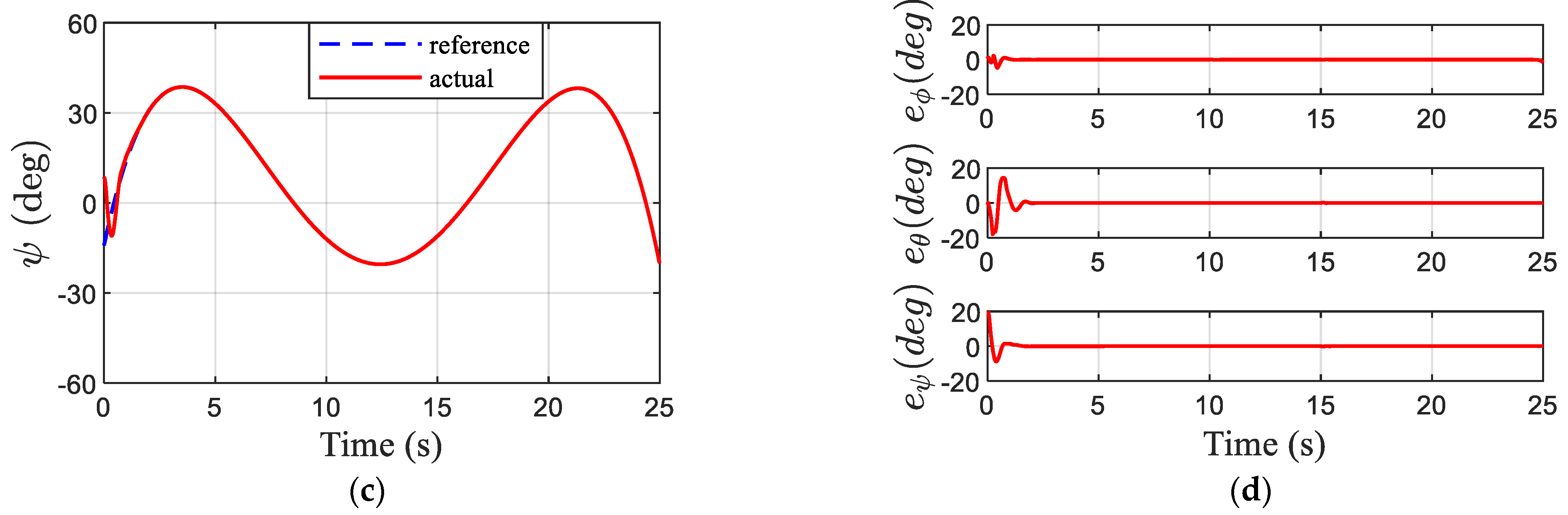
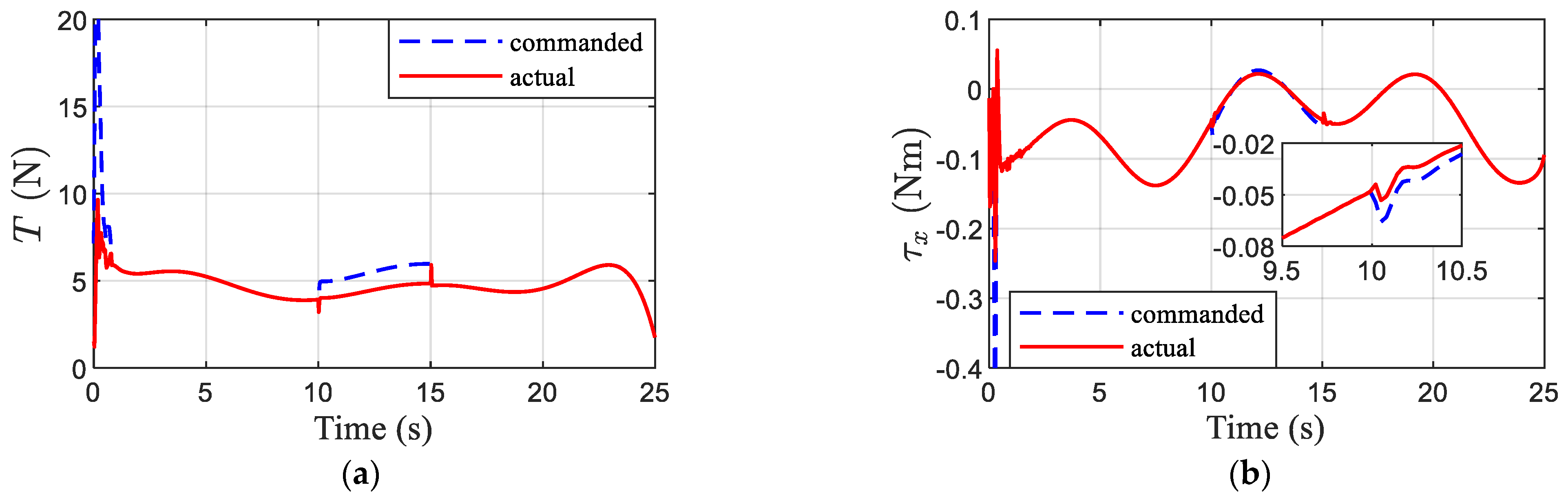
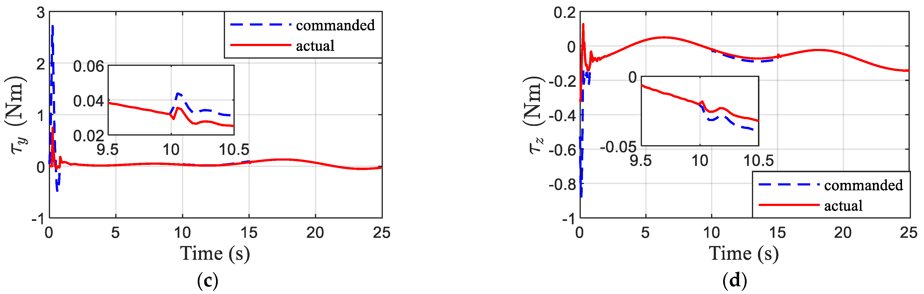
4.1. Simulation Results

The parameters of the QUAV are given as $m=0.5 \mathrm{kg}$, $g=9.8 {\mathrm{m}/\mathrm{s}}^2$, $c_T=2.98\times {10}^{-6}$, $c_M=1.14\times {10}^{-7}$, $d=0.225 \mathrm{m}$, $J={10}^{-3}\times \mathrm{diag}\left[\begin{array}{ccc}4.9& 4.9& 8.8\end{array}\right] \mathrm{kg}\cdot {\mathrm{m}}^2$, $J_0={10}^{-3}\times \mathrm{diag}\left[\begin{array}{ccc}4.5& 4.5& 8\end{array}\right] \mathrm{kg}\cdot {\mathrm{m}}^2$. The health condition of actuators is represented as

$$\{\begin{array}{l}{\rho }_1={\rho }_2={\rho }_3={\rho }_4=1\hspace{0.17em}\hspace{0.17em}\hspace{1em}\hspace{1em}\hspace{1em}0\le t<10\\ {\rho }_1={\rho }_2={\rho }_3={\rho }_4=0.9\hspace{0.17em},\hspace{1em}\hspace{1em}10\le t\le 15\\ {\rho }_1={\rho }_2={\rho }_3={\rho }_4=1,\hspace{0.17em}\hspace{0.17em}\hspace{1em}\hspace{1em}\hspace{1em}t>15\end{array}$$

(54)

In fact, the saturation limit of rotor speed is influenced in the case of actuator faults, so it can be set as

$${\varpi }_{\max i}=\{\begin{array}{l}\delta {\overline{\varpi }}_{\max i},\hspace{1em}\hspace{1em}\mathrm{with}\hspace{0.17em}\mathrm{actuator}\hspace{0.17em}\mathrm{faults}\\ {\overline{\varpi }}_{\max i},\hspace{1em}\hspace{1em}\hspace{0.17em}\hspace{0.17em}\mathrm{without}\hspace{0.17em}\mathrm{actuator}\hspace{0.17em}\mathrm{faults}\end{array}$$

(55)

where $\delta$ is determined by the actual situation and is set to $\delta =0.9$, and ${\overline{\varpi }}_{\max i}$ represents the saturation limit without actuator faults, ${\overline{\varpi }}_{\max 1}={\overline{\varpi }}_{\max 2}={\overline{\varpi }}_{\max 3}={\overline{\varpi }}_{\max 4}=900 \mathrm{rpm}$.

The external disturbances of the translational and rotational subsystem are supposed to be

$${\Delta }_1=0.1\times \left[\begin{array}{c}1+\sin (0.3t)+\cos (0.8t)\\ -1+\sin (0.6t)-\cos (0.4t)\\ 1+\sin (0.5t)+\cos (0.2t)\end{array}\right]\mathrm{N}/\mathrm{kg}$$

(56)

$${\Delta }_2=0.05\times \left[\begin{array}{c}1+\sin (0.3t)+\cos (0.8t)\\ -1+\sin (0.6t)-\cos (0.4t)\\ 1+\sin (0.5t+\pi /2)+\cos (0.2t+\pi /2)\end{array}\right]\mathrm{Nm}$$

(57)

The parameters of fixed-time tracking controller and fixed-time UIO for the translational subsystem are set as $k_p=0.3$, $k_v=0.9$, $\alpha =0.8$, $m_1=0.8$, $n_1=1.2$, $L_1=\mathrm{diag}\left[\begin{array}{ccc}50& 50& 50\end{array}\right]$, $L_2=H_1=H_2=\mathrm{diag}\left[\begin{array}{ccc}1& 1& 1\end{array}\right]$.

The parameters of the fixed-time tracking controller and fixed-time UIO for rotational subsystem are set as $k_1=80$, $k_2=10$, $a=0.8$, $m_2=0.8$, $n_2=1.2$, $L_3=\mathrm{diag}\left[\begin{array}{ccc}40& 40& 40\end{array}\right]$, $L_4=H_3=H_4=\mathrm{diag}\left[\begin{array}{ccc}1& 1& 1\end{array}\right]$.

The tracking results of position and speed are presented in Figure 3, where $V=\sqrt{u^2+v^2+w^2}$. Figure 4 shows the trajectory tracking results from 3D view and X-Y view. Obviously, the proposed fixed-time tracking controller for the translational subsystem can track the desired command accurately. Figure 5 presents the simulation results of the Euler angle and its tracking error, and we can conclude that the tracking performance of the designed fixed-time tracking controller for the rotational subsystem is satisfactory, and the tracking error could rapidly converge to zero. The rotor speed commanded by the controller and the actual rotor speed are presented in Figure 6, and we can see that the commanded rotor speed increases in order to track the desired command in the event of actuator faults. The saturation limit of rotor speed decreases during actuator faults. Furthermore, even though the controller orders a high rotor speed, the actual rotor speed does not surpass the saturation limit we set. Figure 7 depicts the controller’s commanded thrust and torque as well as the actual thrust and torque. The thrust and torque commanded, as well as the actual thrust and torque, are different due to the difference between the commanded rotor speed and the actual rotor speed at the start and in the case of actuator faults. The estimation results of lumped disturbances for both translational and rotational subsystem are drawn in Figure 8, and the observation performance of the proposed fixed-time UIO is acceptable. Though the lumped disturbances are very large at first, which is caused by the fact that the actual rotor speed does not match the commanded rotor speed in the starting stage, the proposed fixed-time UIO can estimate the lumped disturbances quickly and precisely.

4.2. Comparison

To verify the performance of the proposed fixed-time UIO (FUIO), simulations using the fixed-time extend state observer (FESO) in [22] and the fixed-time integral sliding mode disturbance observer (FISMDO) in [25] are carried out for comparison.

The FESO for rotational subsystem is designed as

$$\{\begin{array}{c}\dot{\hat{\Theta }}=\hat{M}+p_{1}si{g}^{m_3}({\xi }_1)+q_{1}si{g}^{n_3}({\xi }_1)\hfill \\ \dot{\hat{M}}=W{J}_0^{-1}{\tau }_c+\hat{D}+p_{2}si{g}^{m_4}({\xi }_1)+q_{2}si{g}^{n_4}({\xi }_1)\hfill \\ \dot{\hat{D}}=p_{3}si{g}^{m_5}({\xi }_1)+q_{3}si{g}^{n_5}({\xi }_1)+{\gamma }_{1}sign({\xi }_1)\hfill \end{array}$$

(58)

where ${\xi }_1=\Theta -\hat{\Theta }$, $\hat{\Theta },\hat{M},\hat{D}$ are the estimations of $\Theta ,M,D$, respectively. The parameters are set as $m_3=0.7$, $m_4=2m_3-1$, $m_5=3m_3-2$, $n_3=1.2$, $n_4=2n_3-1$, $n_5=3n_3-2$, $p_1=q_1=10$, $p_2=q_2=27$, $p_3=q_3=74$, ${\gamma }_1=3>\Vert \dot{D}\Vert$.

The FESO for translational subsystem is designed as

$$\{\begin{array}{c}\dot{\hat{p}}=\hat{v}+p_{4}si{g}^{m_6}({\xi }_2)+q_{4}si{g}^{n_6}({\xi }_2)\hfill \\ \dot{\hat{v}}=u_c+\hat{d}+p_{5}si{g}^{m_7}({\xi }_2)+q_{5}si{g}^{n_7}({\xi }_2)\hfill \\ \dot{\hat{d}}=p_{6}si{g}^{m_8}({\xi }_2)+q_{6}si{g}^{n_8}({\xi }_2)+{\gamma }_{2}sign({\xi }_2)\hfill \end{array}$$

(59)

where ${\xi }_2=p-\hat{p}$, $\hat{p},\hat{v},\hat{d}$ are the estimations of $p,v,d$, respectively. The parameters are given as $m_6=0.8$, $m_7=2m_6-1$, $m_8=3m_6-2$, $n_6=1.2$, $n_7=2n_6-1$, $n_8=3n_6-2$, $p_4=q_4=10$, $p_5=q_5=27$, $p_6=q_6=15$, ${\gamma }_2=1>\Vert \dot{d}\Vert$.

The FISMDO for the rotational subsystem is designed as

$$\{\begin{array}{c}{\dot{s}}_0=D-\hat{D}\hfill \\ s_1={\dot{s}}_0+{\displaystyle \int \left[{\lambda }_1{\lceil s_0\rfloor }^{a_3}+{\lambda }_2{\lceil s_0\rfloor }^{b_3}+{\lambda }_3{\lceil {\dot{s}}_0\rfloor }^{a_4}+{\lambda }_4{\lceil {\dot{s}}_0\rfloor }^{b_4}\right]\mathrm{d}s}\hfill \\ \dot{\hat{D}}={\lambda }_1{\lceil s_0\rfloor }^{a_3}+{\lambda }_2{\lceil s_0\rfloor }^{b_3}+{\lambda }_3{\lceil {\dot{s}}_0\rfloor }^{a_4}+{\lambda }_4{\lceil {\dot{s}}_0\rfloor }^{b_4}\hfill \\ \hspace{1em}\hspace{1em}+{\lambda }_5{\lceil s_1\rfloor }^{a_5}+{\lambda }_6{\lceil s_1\rfloor }^{b_5}+{\gamma }_3\mathrm{sgn}(s_1)\hfill \end{array}$$

(60)

where ${\lambda }_1={\lambda }_3=2$, ${\lambda }_2={\lambda }_4=4$, ${\lambda }_5={\lambda }_6=0.5$, $a_3=a_4=a_5=0.8$, $b_3=b_4=b_5=1.2$, ${\gamma }_3=3>\Vert \dot{D}\Vert$.

The FISMDO for the translational subsystem is designed as

$$\{\begin{array}{c}{\dot{s}}_2=d-\hat{d}\hfill \\ s_3={\dot{s}}_2+{\displaystyle \int \left[{\kappa }_1{\lceil s_2\rfloor }^{a_6}+{\kappa }_2{\lceil s_2\rfloor }^{b_6}+{\kappa }_3{\lceil {\dot{s}}_2\rfloor }^{a_7}+{\kappa }_4{\lceil {\dot{s}}_2\rfloor }^{b_7}\right]\mathrm{d}s}\hfill \\ \dot{\hat{d}}={\kappa }_1{\lceil s_2\rfloor }^{a_6}+{\kappa }_2{\lceil s_2\rfloor }^{b_6}+{\kappa }_3{\lceil {\dot{s}}_2\rfloor }^{a_7}+{\kappa }_4{\lceil {\dot{s}}_2\rfloor }^{b_7}\hfill \\ \hspace{1em}\hspace{1em}+{\kappa }_5{\lceil s_3\rfloor }^{a_8}+{\kappa }_6{\lceil s_3\rfloor }^{b_8}+{\gamma }_4\mathrm{sgn}(s_3)\hfill \end{array}$$

(61)

where ${\kappa }_1={\kappa }_3=2$, ${\kappa }_2={\kappa }_4=4$, ${\kappa }_5={\kappa }_6=0.5$, $a_6=a_7=a_8=0.8$, $b_6=b_7=b_8=1.2$, ${\gamma }_4=1>\Vert \dot{d}\Vert$.

Figure 9 depicts the estimation error of lumped disturbances, employing three observers for translational and rotational subsystems. Obviously, the estimation error of the three observers could converge to zero. However, the estimation performance of the three observers is also different. Compared with FESO, the estimation error converges faster when using the FUIO and the FISMDO to estimate the lumped disturbances. Moreover, according to Figure 9c, we can find that the FUIO converges fastest when the lumped disturbance changes abruptly owing to actuator faults. Additionally, since the FUIO does not include the sign function, its estimation error converges more smoothly and accurately than the FESO and FISMDO. The tracking error of the position and the Euler angle when using different disturbance observers are shown in Figure 10, and we find that the convergence speed of tracking error is faster in the case of actuator faults and the tracking precision is higher when using the FUIO because it has better estimation performance.

Remark 3.

When the rotor speed saturation is considered, the lumped disturbance is very large. For ease of analysis, the rotor speed saturation is not considered in the comparison simulations.

Remark 4.

As the estimation precision of the disturbance observer can affect the lumped disturbance, the lumped disturbance is different when using different observers to estimate the lumped disturbance. Hence, we compare the estimation performance of the three observers using the estimation error.

Remark 5.

From Equations (58)–(61), we know that the FESO and FISMDO are designed based on the boundary of the derivative of the lumped disturbance. Therefore, the estimation performance of the FESO and FISMDO cannot be guaranteed in theory when the lumped disturbance changes sharply.

Remark 6.

According to the estimation error of different observers presented in Figure 9, we can conclude the advantages of the FUIO. First, the sign function is absent in FUIO, so there is no chattering and the estimation precision is higher. Additionally, the design process of FUIO does not need prior knowledge of the boundary of the disturbance or its derivative. Therefore, the design process becomes easier and the application is expanded. Moreover, the FUIO can observe the lumped disturbance accurately and quickly when the lumped disturbance changes suddenly due to actuator faults.

4.3. Discussion

4.3.1. Differences between Rotor Speed Saturation and Thrust or Torque Saturation

In contrast with [29,30,31], the rotor speed saturation is considered in this paper instead of thrust and torque saturation. According to Equation (8), we find that the total thrust is related to the rotor speed of all four motors. Therefore, as soon as the rotor speed of any of the motors reaches saturation, the total thrust will be affected. When only thrust saturation is considered, the role of each rotor speed cannot be reflected. Hence, rotor speed saturation is considered in this paper, which is more reasonable.

4.3.2. The Feature of Proposed Observer

In the process of observer design, a new state $\mathsf{\eta }$ is introduced in Equation (24), and its time derivative in Equation (25) shows that the new state $\mathsf{\eta }$ is the first-order filtering of lumped disturbance $d$. Using the new state, the observer is designed in Equation (26). Instead of estimating the lumped disturbance directly, the observer first observes the new state and then uses the filtering relationship between the disturbance and the new state to estimate the disturbance. The advantage of this is that the upper bound of the derivative of lumped disturbance is not required and the lumped disturbance can be estimated accurately when it changes suddenly.

4.3.3. The Future Work

In this section, simulation results that consider the external disturbance, inertia uncertainties, actuator faults, and input saturation are presented to validate the effectiveness and superiority of the proposed control scheme. Although the simulation results are satisfactory, the flight experiment verification is also indispensable, which we will explore in future work.

5. Conclusions

This paper investigates the trajectory tracking control problem for a QUAV in the presence of external disturbances, inertia uncertainties, actuator faults, and input saturation. The simulation results show that the high-accuracy estimation of the lumped disturbance can be obtained in fixed time, employing the proposed fixed-time UIO. Compared with other observers, such as the observers in [20,21,22,23,24,25,26], the advantages of proposed fixed-time UIO can be summarized as follows: (a) there is no chattering in the estimation of lumped disturbance and the estimation precision is better; (b) prior knowledge of the boundary of the disturbance or its derivative is not required; (c) the lumped disturbance can be observed accurately and quickly when it changes suddenly due to actuator faults. The fixed-time tracking controllers for translational and rotational subsystems could drive the tracking error into a small region in fixed time regardless of the initial values with the help of the proposed fixed-time UIO. Rigorous convergence analysis and numerical simulation results have demonstrated the effectiveness and superiority of the proposed control scheme.

References

1. Serrano, M.E.; Gandolfo, D.C.; Scaglia, G.J.E. Trajectory tracking controller for unmanned helicopter under environmental disturbances. ISA Trans. 2020, 106, 171–180. [Google Scholar] [CrossRef] [PubMed]
2. Cao, C.Y.; Wei, C.S.; Liao, Y.X.; Zhang, Y.C.; Li, J. On novel trajectory tracking control of quadrotor UAV: A finite-time guaranteed performance approach. J. Franklin Inst. 2022, 359, 8454–8483. [Google Scholar] [CrossRef]
3. Li, B.; Song, C.; Bai, S.X.; Huang, J.Y.; Ma, R.; Wan, K.F.; Neretin, E. Multi-UAV trajectory planning during cooperative tracking based on a Fusion Algorithm integrating MPC and standoff. Drones 2023, 7, 196. [Google Scholar] [CrossRef]
4. Kidambi, K.B.; Fermuller, C.; Aloimonos, Y.; Xu, H. Robust nonlinear control-based trajectory tracking for quadrotors under uncertainty. IEEE Control Syst. Lett. 2021, 5, 2042–2047. [Google Scholar] [CrossRef]
5. Blas, L.A.; Davila, J.; Salazar, S.; Bonilla, M. Robust trajectory tracking for an uncertain UAV based on active disturbance rejection. IEEE Control Syst. Lett. 2022, 6, 1466–1471. [Google Scholar] [CrossRef]
6. Singhal, K.; Kumar, V. Robust trajectory tracking control of non-holonomic wheeled mobile robots using an adaptive fractional order parallel fuzzy PID controller. J. Franklin Inst. 2022, 359, 4160–4215. [Google Scholar] [CrossRef]
7. Mathiyalagan, K.; Sangeetha, G. Finite-time stabilization of nonlinear time delay systems using LQR based sliding mode control. J. Franklin Inst. 2019, 356, 3948–3964. [Google Scholar] [CrossRef]
8. Lee, D.; Kim, H.J.; Sastry, S. Feedback linearization vs. adaptive sliding mode control for a quadrotor helicopter. Int. J. Control Autom. Syst. 2009, 7, 419–428. [Google Scholar] [CrossRef]
9. Koksal, N.; An, H.; Fidan, B. Backstepping-based adaptive control of a quadrotor UAV with guaranteed tracking performance. ISA Trans. 2020, 105, 98–110. [Google Scholar] [CrossRef] [PubMed]
10. Liu, W.Q.; Cheng, X.H.; Zhang, J.J. Command filter-based adaptive fuzzy integral backstepping control for quadrotor UAV with input saturation. J. Franklin Inst. 2023, 360, 484–507. [Google Scholar] [CrossRef]
11. Labbadi, M.; Boukal, Y.; Cherkaoui, M.; Djemai, M. Fractional-order global sliding mode controller for an uncertain quadrotor UAVs subjected to external disturbances. J. Franklin Inst. 2021, 358, 4822–4847. [Google Scholar] [CrossRef]
12. Labbadi, M.; Cherkaoui, M. Adaptive fractional-order nonsingular fast terminal sliding mode based robust tracking control of quadrotor UAV with Gaussian random disturbances and uncertainties. IEEE Trans. Aerosp. Electron. Syst. 2021, 57, 2265–2277. [Google Scholar] [CrossRef]
13. Wang, Q.; Wang, W.; Suzuki, S.; Namiki, A.; Liu, H.X.; Li, Z.R. Design and implementation of UAV velocity controller based on reference model sliding mode control. Drones 2023, 7, 130. [Google Scholar] [CrossRef]
14. Huang, D.Q.; Huang, T.P.; Qin, N.; Li, Y.A.; Yang, Y. Finite-time control for a UAV system based on finite-time disturbance observer. Aerosp. Sci. Technol. 2022, 129, 107825. [Google Scholar] [CrossRef]
15. Cheng, W.L.; Jiang, B.; Zhang, K.; Ding, S.X. Robust finite-time cooperative formation control of UGV-UAV with model uncertainties and actuator faults. J. Franklin Inst. 2021, 358, 8811–8837. [Google Scholar] [CrossRef]
16. Wang, J.H.; Alattas, K.A.; Bouteraa, Y.; Mofid, O.; Mobayen, S. Adaptive finite-time backstepping control tracker for quadrotor UAV with model uncertainty and external disturbance. Aerosp. Sci. Technol. 2023, 133, 108088. [Google Scholar] [CrossRef]
17. Liu, B.J.; Li, A.J.; Guo, Y.; Wang, C.Q. Adaptive distributed finite-time formation control for multi-UAVs under input saturation without collisions. Aerosp. Sci. Technol. 2022, 120, 107252. [Google Scholar] [CrossRef]
18. Xia, K.W.; Son, H.S. Adaptive fixed-time control of autonomous VTOL UAVs for ship landing operations. J. Franklin Inst. 2020, 357, 6175–6196. [Google Scholar] [CrossRef]
19. Tan, J.; Dong, Y.F.; Shao, P.Y.; Qu, G.M. Anti-saturation adaptive fault-tolerant control with fixed-time prescribed performance for UAV under AOA asymmetric constraint. Aerosp. Sci. Technol. 2022, 120, 107264. [Google Scholar] [CrossRef]
20. Cui, L.; Hou, X.Y.; Zuo, Z.Q.; Yang, H.J. An adaptive fast super-twisting disturbance observer-based dual closed-loop attitude control with fixed-time convergence for UAV. J. Franklin Inst. 2022, 359, 2514–2540. [Google Scholar] [CrossRef]
21. Chen, L.L.; Liu, Z.B.; Dang, Q.Q.; Zhao, W.; Wang, G.D. Robust trajectory tracking control for a quadrotor using recursive sliding mode control and nonlinear extended state observer. Aerosp. Sci. Technol. 2022, 128, 107749. [Google Scholar] [CrossRef]
22. Shao, S.S.; Wang, S.; Zhao, Y.J. Fixed time output feedback control for quadrotor unmanned aerial vehicle under disturbances. Proc. Inst. Mech. Eng. Part G J. Aerosp. Eng. 2022, 236, 3554–3566. [Google Scholar] [CrossRef]
23. Cui, L.; Zhang, R.Z.; Yang, H.J.; Zuo, Z.Q. Adaptive super-twisting trajectory tracking control for an unmanned aerial vehicle under gust winds. Aerosp. Sci. Technol. 2021, 115, 106833. [Google Scholar] [CrossRef]
24. Gonzalez, J.A.C.; Pena, O.S.; Morales, J.D.L. Observer-based super twisting design: A comparative study on quadrotor altitude control. ISA Trans. 2021, 109, 307–314. [Google Scholar] [CrossRef] [PubMed]
25. Su, B.; Wang, H.B.; Wang, Y.L. Dynamic event-triggered formation control for AUVs with fixed-time integral sliding mode disturbance observer. Ocean Eng. 2021, 240, 109893. [Google Scholar] [CrossRef]
26. Dong, Z.; Liu, L.; Wang, S.P. Sliding mode disturbance observer-based adaptive dynamic inversion fault-tolerant control for Fixed-Wing UAV. Drones 2022, 6, 295. [Google Scholar] [CrossRef]
27. Xuan-Mung, N.; Golestani, M. Energy-efficient disturbance observer-based attitude tracking control with fixed-time convergence for spacecraft. IEEE. Trans. Aero. Elec. Syst. 2022, 1–10. [Google Scholar] [CrossRef]
28. Xiong, C.G.; Yang, L.; Zhou, B.; Chen, Y. Finite-time fault-tolerant control of robotic systems with uncertain dynamics. Int. J. Control Autom. Syst. 2022, 20, 2681–2690. [Google Scholar] [CrossRef]
29. Fu, C.Y.; Tian, Y.T.; Huang, H.Y.; Zhang, L.; Peng, C. Finite-time trajectory tracking control for a 12-rotor unmanned aerial vehicle with input saturation. ISA Trans. 2018, 81, 52–62. [Google Scholar] [CrossRef]
30. Liu, K.; Wang, R.J.; Wang, X.D.; Wang, X.X. Anti-saturation adaptive finite-time neural network based fault-tolerant tracking control for a quadrotor UAV with external disturbances. Aerosp. Sci. Technol. 2021, 115, 106790. [Google Scholar] [CrossRef]
31. Cao, N.; Lynch, A.F. Inner-outer loop control for quadrotor UAVs with input and state constraints. IEEE Trans. Contr. Syst. T 2015, 24, 1797–1804. [Google Scholar] [CrossRef]
32. Lee, D. Fault-tolerant finite-time controller for attitude tracking of rigid spacecraft using intermediate quaternion. IEEE Trans. Aero Elec Sys. 2021, 57, 540–553. [Google Scholar] [CrossRef]
33. Polyakov, A. Nonlinear feedback design for fixed-time stabilization of linear control system. IEEE Trans. Automat Contr. 2012, 57, 2106–2110. [Google Scholar] [CrossRef]
34. Bernuau, E.; Efimov, D.; Perruquetti, W. On homogeneity and its application in sliding mode control. J. Franklin Inst. 2014, 351, 1866–1901. [Google Scholar] [CrossRef]
35. Andrieu, V.; Praly, L.; Astolfi, A. Homogeneous approximation, recursive observer design, and output feedback. SIAM J. Control Optim. 2009, 47, 1814–1850. [Google Scholar] [CrossRef]
Figure 1. The framework of QUAV.
Drones 07 00344 g001
Figure 2. Control block diagram of the proposed control method.
Drones 07 00344 g002
Figure 3. Position and speed of QUAV: (a) position x ; (b) position y ; (c) position z ; (d) speed.
Drones 07 00344 g003
Figure 4. Three-dimensional trajectory of QUAV: (a) 3D view; (b) X-Y view.
Drones 07 00344 g004
Figure 5. Euler angle and its tracking error: (a) Roll angle; (b) pitch angle; (c) yaw angle; (d) error.
Drones 07 00344 g005aDrones 07 00344 g005b
Figure 6. Rotor speed: (a) Rotor 1; (b) rotor 2; (c) rotor 3; (d) rotor 4.
Drones 07 00344 g006
Figure 7. Thrust and torque: (a) thrust; (b) torque-X; (c) torque-Y; (d) torque-Z.
Drones 07 00344 g007aDrones 07 00344 g007b
Figure 8. Observation results of lumped disturbances: (a) disturbance d x ; (b) disturbance d y ; (c) disturbance d z ; (d) disturbance D x ; (e) disturbance D y ; (f) disturbance D z .
Drones 07 00344 g008
Figure 9. Estimation error of lumped disturbances: (a) error of dx; (b) error of d y ; (c) error of d z ; (d) error of D x ; (e) error of D y ; (f) error of D z .
Drones 07 00344 g009
Figure 10. Tracking error of position and Euler angle: (a) error of x ; (b) error of y ; (c) error of z ; (d) error of ϕ ; (e) error of θ ; (f) error of ψ .
Drones 07 00344 g010
Disclaimer/Publisher’s Note: The statements, opinions and data contained in all publications are solely those of the individual author(s) and contributor(s) and not of MDPI and/or the editor(s). MDPI and/or the editor(s) disclaim responsibility for any injury to people or property resulting from any ideas, methods, instructions or products referred to in the content.