Figure 1.
Description of Perspective–n–Point (PnP) Algorithm. The objective of the algorithm is to determine the relative rotation and translation between the reference frame and the camera frame. represents one of the object points in the reference coordinate system. represents the corresponding image point of in the normalized camera frame.
Figure 2.
The patterns of Augmented Reality University of Cordoba (ArUco) marker. The sequence of marker patterns’ ID from left to right is 0∼5.
Figure 2.
The patterns of Augmented Reality University of Cordoba (ArUco) marker. The sequence of marker patterns’ ID from left to right is 0∼5.
Figure 3.
A pipeline of the proposed algorithm consists of two components, robust orientation estimator (yellow part) and measurement of sensor orientation (blue part). Only the stereo camera’s left eye is utilized in the online measurement procedure.
Figure 3.
A pipeline of the proposed algorithm consists of two components, robust orientation estimator (yellow part) and measurement of sensor orientation (blue part). Only the stereo camera’s left eye is utilized in the online measurement procedure.
Figure 4.
An overview of the coordinate system used in this paper.
Figure 4.
An overview of the coordinate system used in this paper.
Figure 5.
A schematic of geomagnetic vector rotation. To determine the heading angle uniquely, we rotate about the z-axis of the reference frame in the YOZ plane to obtain .
Figure 5.
A schematic of geomagnetic vector rotation. To determine the heading angle uniquely, we rotate about the z-axis of the reference frame in the YOZ plane to obtain .
Figure 6.
A pipeline of proposed estimator.
Figure 6.
A pipeline of proposed estimator.
Figure 7.
A pipeline of the proposed method for orientation measurement. The proposed method involves offline calibration and online measurement steps. The segment on offline calibration consists of two steps: calibration of markers and calibration of hand–eye.
Figure 7.
A pipeline of the proposed method for orientation measurement. The proposed method involves offline calibration and online measurement steps. The segment on offline calibration consists of two steps: calibration of markers and calibration of hand–eye.
Figure 8.
A pinhole model of the camera. The camera model specifies the projection relationship between object points in the reference frame and image points in the pixel frame.
Figure 8.
A pinhole model of the camera. The camera model specifies the projection relationship between object points in the reference frame and image points in the pixel frame.
Figure 9.
The overview of Base Cube, which is used as a measurement standard. (a,b) depict the placement of six ArUco markers on the outer surface, while (c) depicts the calibrated path and associated variables. The calibration objective is to identify the five relative rotations in .
Figure 9.
The overview of Base Cube, which is used as a measurement standard. (a,b) depict the placement of six ArUco markers on the outer surface, while (c) depicts the calibrated path and associated variables. The calibration objective is to identify the five relative rotations in .
Figure 10.
A schematic depiction of the hand–eye calibration method. We obtain along two distinct paths (red path and blue path) and formulate the least squares problem in order to solve . The yellow gradient arrow in the figure represents the timeline, and the timeline’s vertical trajectory represents the same period.
Figure 11.
The hardware experiment environment. The MPU9250 (right sub-image) sensor is mounted on an orthogonal reference bracket within the Base Cube. The left sub-image shows the Raspberry4B computer.
Figure 11.
The hardware experiment environment. The MPU9250 (right sub-image) sensor is mounted on an orthogonal reference bracket within the Base Cube. The left sub-image shows the Raspberry4B computer.
Figure 12.
Image samples of the test set used for calibration of adjacent markers. The subgraphs (a∼e) represent randomly selected patterns from videos of test sets V02, V03, V04, V05, and V21, respectively. The test set names correspond to the subscripts of the variables in .
Figure 12.
Image samples of the test set used for calibration of adjacent markers. The subgraphs (a∼e) represent randomly selected patterns from videos of test sets V02, V03, V04, V05, and V21, respectively. The test set names correspond to the subscripts of the variables in .
Figure 13.
The performance comparison of PnP algorithms. The PnP algorithm is used to generate data pairings to calibrate adjacent markers. This figure depicts the pixel coordinate distribution of re–projection error for each ArUco marker in five test videos utilizing the participating P3P, DLT, and EPnP algorithms. Each vertical column represents the V02, V03, V04, V05, and V21 test sets. The effects of the P3P, DLT, and EPnP algorithms are depicted from left to right. The regions within the red circle represent regions with a 1-pixel re–projection error. The points of different colors in the scatterplot section are to distinguish adjacent points.
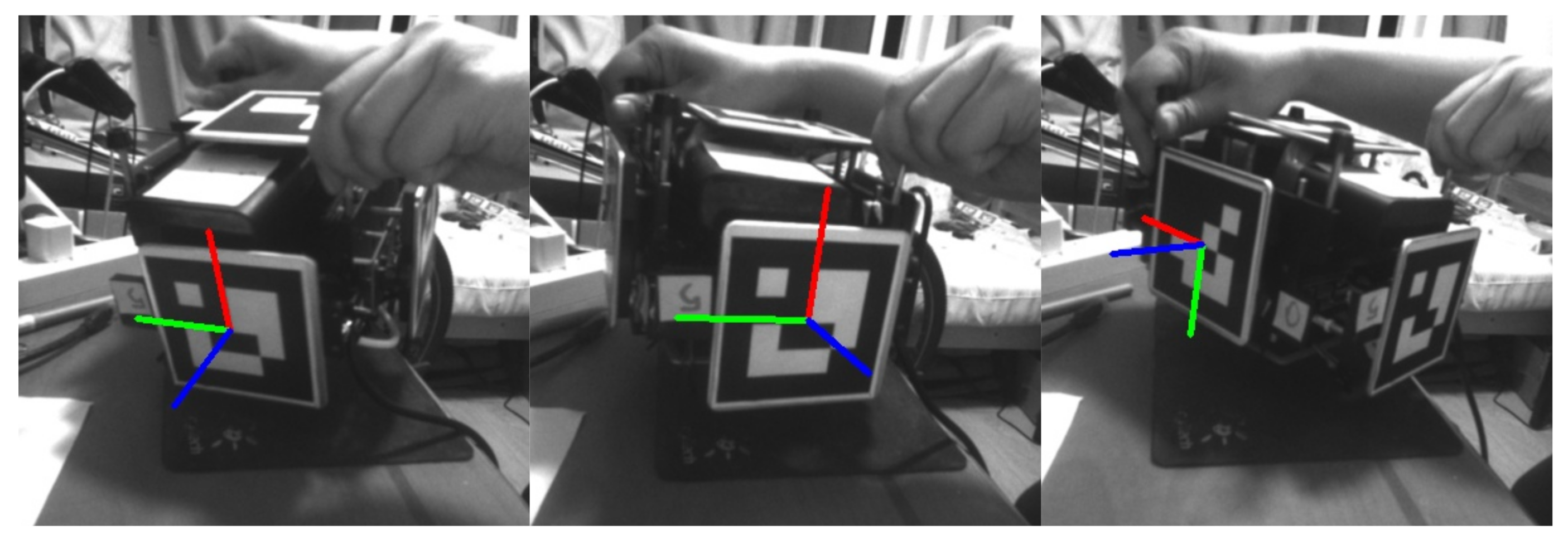
Figure 14.
The visualization of hand–eye calibration.
Figure 14.
The visualization of hand–eye calibration.
Figure 15.
The error results of hand–eye calibration. The left, center, and right images depict the angle errors following roll, pitch, and yaw calibration, respectively.
Figure 15.
The error results of hand–eye calibration. The left, center, and right images depict the angle errors following roll, pitch, and yaw calibration, respectively.
Figure 16.
The distribution of visual measurement orientation re–projection error. (a,b) represent the statistical information of the re-projection error of two image sequences (low–dynamic and high–dynamic) utilized to evaluate the orientation estimation algorithms. The scatter plot illustrates the distribution of re–projection error points within the pixel plane. The points of different colors in the scatterplot section are to distinguish adjacent points.
Figure 17.
A comparison of orientation estimation results under low–dynamic conditions.
Figure 17.
A comparison of orientation estimation results under low–dynamic conditions.
Figure 18.
A comparison of orientation errors in Euler angle under low–dynamic conditions. Each row from top to bottom represents the test result of ESKF, Madgwick filter, Mahony filter, and proposed estimator. Each column from left to right displays the comparison results for roll, pitch, and yaw angle in that order.
Figure 19.
A comparison of orientation estimation results in under high–dynamic conditions.
Figure 19.
A comparison of orientation estimation results in under high–dynamic conditions.
Figure 20.
A comparison of orientation errors in Euler angle under high–dynamic conditions. Each row from top to bottom represents the test result of ESKF, Madgwick filter, Mahony filter, and proposed estimator. Each column from left to right displays the comparison results for roll, pitch, and yaw angle in that order.
Table 1.
The declarations of symbols and rules.
Table 1.
The declarations of symbols and rules.
| Symbols | Description |
|---|
| Bold capital letters represent matrices |
| Bold lowercase letters represent vectors |
| x | Scalar |
| Measurement value of sensor |
| Probability |
| Normalized quaternion |
| The imaginary part of a quaternion |
| Optimal value |
| Coordinate system |
Table 2.
The results of adjacent markers calibration.
Table 2.
The results of adjacent markers calibration.
| Test Sets | Algorithm | () | () | |
|---|
| V02 | P3P + LM | 0.14 | 0.12 | |
| P3P + DL | 0.14 | 0.05 |
| DLT + LM | 0.52 | 0.09 |
| DLT + DL | 0.52 | 0.08 |
| V03 | P3P + LM | 0.27 | 0.13 | |
| P3P + DL | 0.27 | 0.06 |
| DLT + LM | 0.51 | 0.15 |
| DLT + DL | 0.51 | 0.08 |
| V04 | P3P + LM | 0.53 | 0.32 | |
| P3P + DL | 0.53 | 0.06 |
| DLT + LM | 1.22 | 0.21 |
| DLT + DL | 1.22 | 0.08 |
| V05 | P3P + LM | 0.54 | 0.09 | |
| P3P + DL | 0.54 | 0.08 |
| DLT + LM | 1.14 | 0.15 |
| DLT + DL | 1.14 | 0.24 |
| V21 | P3P + LM | 0.38 | 0.09 | |
| P3P + DL | 0.38 | 0.06 |
| DLT + LM | 1.23 | 0.31 |
| DLT + DL | 1.23 | 0.09 |
Table 3.
A comparison of orientation errors under low–dynamic condition (rad).
Table 3.
A comparison of orientation errors under low–dynamic condition (rad).
| Algorithm | | | | | | | | |
|---|
| ESKF | 3.141 | 0.205 | 0.059 | 0.011 | 0.038 | 0.005 | 0.241 | 0.188 |
| Madgwick | 0.470 | 0.130 | 0.094 | 0.013 | 0.067 | 0.001 | 0.266 | 0.081 |
| Mahony | 1.205 | 0.136 | 0.158 | 0.016 | 0.062 | 0.004 | 1.185 | 0.076 |
| Proposed | 0.299 | 0.076 | 0.039 | 0.004 | 0.034 | 0.016 | 0.296 | 0.015 |
Table 4.
A statistical analysis of orientation errors under high–dynamic conditions (rad).
Table 4.
A statistical analysis of orientation errors under high–dynamic conditions (rad).
| Algorithm | | | | | | | | |
|---|
| ESKF | 3.141 | 0.514 | 0.347 | 0.046 | 0.177 | 0.027 | 2.598 | 0.198 |
| Madgwick | 5.995 | 0.299 | 0.450 | 0.044 | 0.359 | 0.014 | 1.169 | 0.168 |
| Mahony | 1.324 | 0.253 | 0.254 | 0.044 | 0.187 | 0.016 | 1.317 | 0.217 |
| proposed | 0.600 | 0.138 | 0.179 | 0.021 | 0.055 | 0.030 | 0.598 | 0.029 |
Table 5.
A comparison of estimation efficiency.
Table 5.
A comparison of estimation efficiency.
| Test Data | Algorithm | (ms) | (ms) | (ms) | (ms) |
|---|
| Low dynamics | ESKF | 0.913 | 24.998 | 0.164 | 0.276 |
| Madgwick | 0.007 | 0.626 | <0.001 | 0.018 |
| Mahony | 0.081 | 3.938 | 0.105 | 0.102 |
| Proposed | 9.781 | 53.269 | 0.102 | 0.109 |
| High dynamics | ESKF | 0.864 | 13.737 | 0.167 | 0.393 |
| Madgwick | 0.008 | 1.231 | <0.001 | 0.008 |
| Mahony | 0.078 | 3.842 | 0.011 | 0.041 |
| Proposed | 22.468 | 78.200 | 2.678 | 9.815 |


