Analysis of Aerodynamic Characteristics of Propeller Systems Based on Martian Atmospheric Environment

Abstract

Compared to detection methods employed by Mars rovers and orbiters, the employment of Mars UAVs presents clear advantages. However, the unique atmospheric conditions on Mars pose significant challenges to the design and operation of such UAVs. One of the primary difficulties lies in the impact of the planet’s low air density on the aerodynamic performance of the UAV’s rotor system. In order to determine the aerodynamic characteristics of the rotor system in the Martian atmospheric environment, a rotor system suitable for the Martian environment was designed under the premise of fully considering the special atmospheric environment of Mars, and the aerodynamic characteristics of the rotor system in the compressible and ultra-low Reynolds number environment were numerically simulated by means of a numerical calculation method. Additionally, a bench experiment was conducted in a vacuum chamber simulating the Martian atmospheric environment, and the aerodynamic characteristics of the UAV rotor system in the Martian environment were analyzed by combining theory and experiments. The feasibility of the rotor system applied to the Martian atmospheric environment was verified, and the first generation of Mars unmanned helicopters was developed and validated via hovering experiments, which thereby yielded crucial data support for the design of subsequent Mars UAV models.

1. Introduction

In the solar system, Mars and Earth have a high degree of similarity, with both having obvious changes in seasons, atmosphere and water. As such, the exploration of Mars is not only conducive to the exploration of the origin of life, but also has a considerable significance in respect of expanding human living space. Peijian Ye and Jing Peng [1] summarized some activities and plans for human deep space exploration, including the exploration of Mars, and introduced the significance and development process of deep space exploration; Weiren Wu and Dengyun Yu [2] elaborated on the development and future key technologies of deep space exploration, and provided a detailed introduction to the exploration process of the moon and Mars. In the past, Mars rovers or orbiters have been used for the exploration of Mars, but both have obvious drawbacks. Since the surface of Mars is full of hills and ravines, which is a major obstacle for rover exploration, there is a considerably limited exploration range and slow exploration speed. With regard to orbiters, due to the high distance from the surface of Mars, there are difficulties in exploring the surface of Mars in-depth. Due to the aforementioned factors, airborne platforms are particularly significant, owing to the higher exploration speed, wider detection range, and broader field of view. Further, areas that are inaccessible to Mars rovers can be accessed, and superior imaging and sensing resolution can be provided compared to orbiters. Anubhav Datta [3] described the necessity of using a Mars unmanned aerial vehicle and described the design of an autonomous rotor vehicle (MARV) for Mars exploration. Thus, when considering such factors comprehensively, the airborne platform appears to be the most efficient means of detection.

Revolutionary changes have taken place in the future of Mars exploration. On 9 April 2021, the American Mars Helicopter “MH” successfully landed on Mars, completed the first test flight of human beings on Mars, and unveiled the new chapter of Mars exploration—Cheng, C. [4]. Ruiz, M.C. [5] and Balaram, J. [6], respectively, described the Mars helicopter “MH” to varying degrees, and based on this, conducted deeper research on the aerodynamic characteristics of the Mars propeller. The 1.8 kg “MH” Mars UAV is an unloaded aerodynamic demonstrator, the main purpose of which is to verify the possibility of flying UAVs in the Martian atmosphere and to facilitate understanding of the basic aeronautics of Mars—this is introduced in Balaram, J.’s [7] article; Pipenberg T.B. [8] described the design and testing process of the Mars helicopter rotor system, including the aerodynamic performance, structural strength, vibration characteristics, control strategy, and environmental adaptability of the rotor. To further scientific exploration, the air dynamic performance of Mars rotor systems needs to be more explored.

In recent years, increasing numbers of countries and institutions have begun to explore Mars UAV systems. Due to the unique atmospheric environment of Mars, the rotor blades of Mars UAVs rotate under low Reynolds numbers and compressible flow conditions, which poses new challenges for the design of Mars rotor systems and is a relatively new field for aerodynamics, with few numerical simulations and experimental data currently available. Takaki et al. [9] simulated and calculated the lift–drag characteristics of various airfoils in the Martian environment and found that the effect of a low Reynolds number on the lift–drag characteristics of airfoils was much greater than that of a Mach number on the lift–drag characteristics of airfoils; Shrestha et al. [10] conducted hovering performance experiments on a 200 g Martian coaxial helicopter propeller in a vacuum chamber, and the quality factor of the propeller at different Reynolds numbers was further explored; Kakeru et al. [11] studied the aerodynamic characteristics of an airfoil in the propeller slipstream at low Reynolds numbers and elucidated the effect of propeller slipstream on the control surface efficiency through aerodynamic measurements and particle image velocimetry measurements; Benjamin et al. [12] presented a detailed description of the rotor system and landing gear system of the MH Mars helicopter; KONING et al. [13] calculated the instability points, laminar separation points, and excess points on the surface of the C81Gen airfoil to approximate the two-dimensional rotor boundary layer state during hovering, and used the results on turbulence modeling in fluid dynamics; Kunz et al. [14], Liu et al. [15], and Bohorquez et al. [16] optimized the propeller airfoil for Re < 10,000 based on the theory of lobe element momentum; Oyama et al. [17] used finite element simulations to conclude that unconventional airfoils with considerably thin airfoil thickness and large airfoil curvature can significantly improve the lift-to-drag ratio and mechanical efficiency of Mars propellers in the Martian atmospheric environment; the Ames Research Center of NASA provided a performance comparison between several low Reynolds number airfoils, finding that the cambered airfoil can outperform conventional airfoils [18]; T. Désert analyzed the effects of Reynolds numbers and Mach numbers on the flow through airfoils in a low Reynolds number compressible flow, and proved the significant effect on flow separation and subsequent wake shape [19].

While the aerodynamics of rotor systems in the Martian atmosphere have been investigated in several studies, most rely on numerical simulations, with few experiments conducted to replicate the vacuum conditions of the Martian environment. Such experiments still fall short in comparison to the distant and unknown Martian environment. In order to further explore the aerodynamic characteristics of the propeller in the Martian atmospheric environment, the special atmospheric environment of Mars was fully considered in the present study. In addition, a lightweight Mars UAV rotor system was designed, and strength and stiffness analyses of the lightweight propeller were combined with finite element software. The method of combining numerical simulation calculations and simulations of the vacuum chamber bench experiments of the Martian atmospheric environment was used to further study the aerodynamic characteristics of the rotor system in the Martian atmospheric environment, analyzed the influence of different Reynolds numbers and Mach numbers on the aerodynamic performance of Mars propellers, and established a Blade Element Theory inflow ratio model for the Martian atmospheric environment, so as to provide more sufficient data support for the design of Mars UAVs.

2. Materials and Methods

2.1. Dynamic Conditions in the Atmospheric Environment of Mars

2.1.1. Martian Atmosphere

Compared with the atmospheric environment of the Earth, the Martian atmospheric environment is undoubtedly much worse in the drone flight environment, posing a significant challenge to the design of Mars UAVs. The atmospheric density of Mars is about 1/80 of that of the Earth, which has been identified as the biggest obstacle to the design of Mars UAV rotor systems. Although the gravity acceleration on Mars is only 1/3 of that of the Earth, the impact of the low air density cannot be offset. At the same time, the sound speed on Mars is much lower than that on Earth, further limiting the tip speed of the propeller and increasing the difficulty of propeller design. The proportion of carbon dioxide in the Martian atmosphere is as high as 95%, but because the thinner atmosphere cannot bind the heat energy of the sun, there is a particularly low temperature on Mars. Notably, the lowest temperature reaches minus 140 °C, while the highest temperature is only 20 °C. Low temperature is another challenge that needs to be considered for Mars UAVs, especially for the electronic components inside, which need to be able to withstand low temperatures and other harsh environments. Moreover, in the design of Mars UAV avionics systems, a thermal insulation system needs to be set up so that the electronic components on the Mars UAV can be properly insulated, and the thermal insulation system needs to consume a lot of electric energy, which greatly shortens the endurance of the Mars UAV. As previously reported, the US “MH” Mars UAV has about 2/3 of the electrical energy for internal system insulation, and only 1/3 of the electrical energy is used for flight. Owing to the condensation and sublimation of the polar CO₂ of Mars, the atmospheric environment on Mars shows seasonal changes. In fact, these comparisons between the Martian and Earth atmospheric environments are presented in Braun, Refs. [20,21] Detailed descriptions were provided in all studies.

Table 1. Characteristics of Martian and Earth’s Atmospheric Environment.

Features	Mars	Earth
Acceleration of gravity (m/s2)	3.72	9.78
Atmospheric pressure (Pa)	756	101,300
Air density (kg/m3)	0.0167	1.22
Mean temperature (°C)	−63	15
Sound velocity (m/s)	227	340
Atmospheric dynamic viscosity (kg/(m·s))	1.289 × 10−5	1.789 × 10−5
Gas constants (J/kg/K)	188	287
Specific heat capacity ratioγ	1.29	1.40
Molar mass (g/mol)	44.01	28.96

presents a comparison of the atmospheric environment characteristics of Mars and Earth.

2.1.2. Air Dynamics under Low Reynolds Numbers

Due to the relatively thin density of the atmosphere on the surface of Mars, a simple calculation of the aerodynamic conditions in the Martian atmospheric environment is needed before the propeller design so that the numerical simulation can be conducted more accurately. The Knudsen number ($Kn$) [22] is the ratio of the mean free path of gas molecules to the characteristic scale. In rarefied gas mechanics, the size of the Knudsen number is often used to determine whether a fluid is suitable for the continuity hypothesis. Generally, in fluid mechanics, when $Kn<0.01$, the flow of gas belongs to a continuous medium flow, and the Navier–Stokes equation can be used. The Knudsen number can be calculated using Equation (1):

$$Kn=\frac{kT}{\sqrt{2}\pi {\sigma }_1{}^{2}PL}$$

(1)

where $k$ is the Boltzmann constant, with a value of $1.3806498\times {10}^{-23}$; T is the thermodynamic temperature; ${\sigma }_1$ is the particle diameter, because 95% of the Martian atmospheric environment is carbon dioxide, so the diameter of carbon dioxide can be used instead of the diameter of the Martian atmosphere example diameter; P is the total pressure; and L is the characteristic length, with the propeller diameter considered here being 1.21 m. The indicators present in the Martian atmosphere suggest that the Knudsen number is significantly below 0.01, indicating that the continuity assumption is applicable to the Martian atmospheric environment.

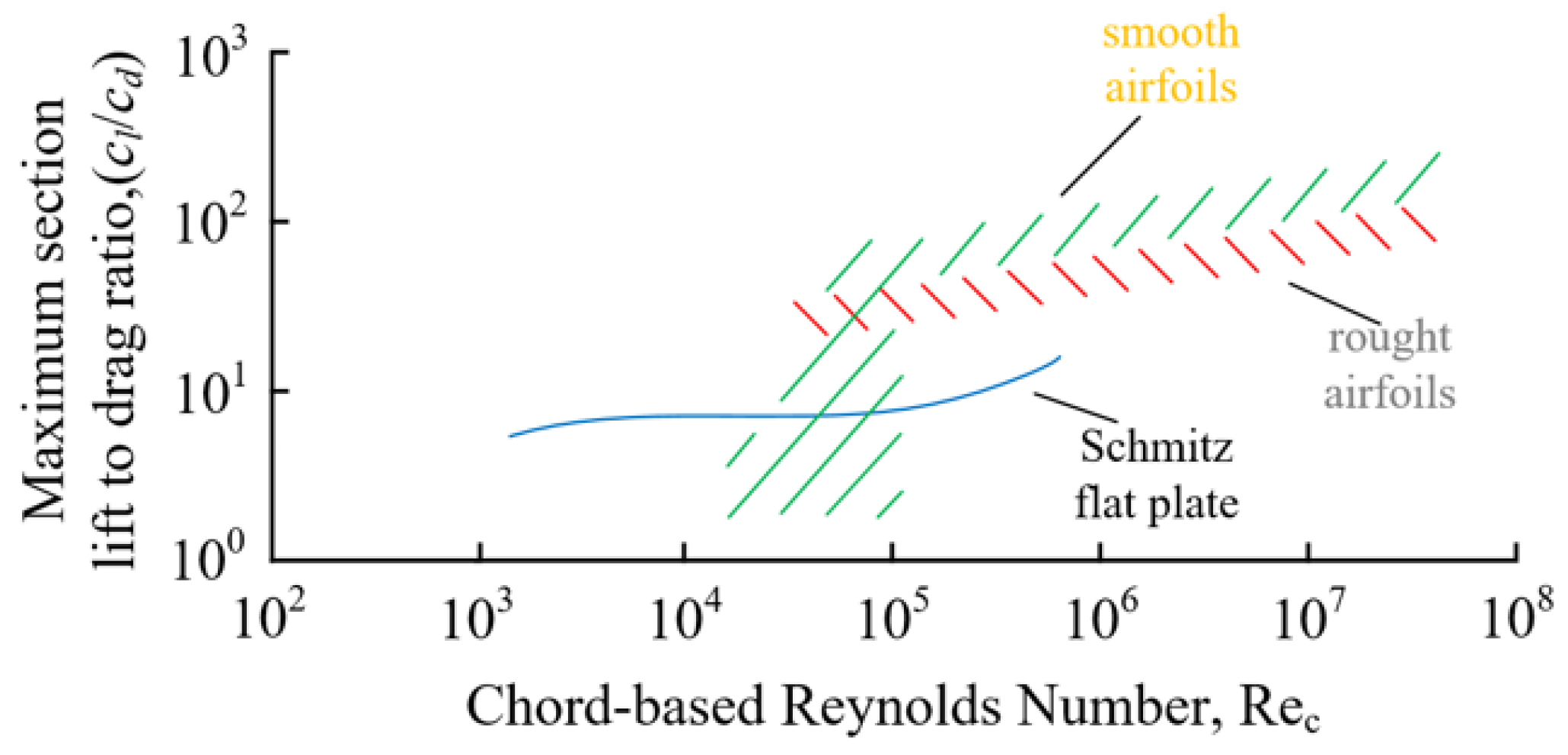
2.1.3. Effect of Reynolds Number on the Aerodynamic Performance of Mars Propellers

The low air density and relatively small rotor size in the Martian atmosphere result in a low Reynolds number for the propeller, and the general chord-based Reynolds number range is Re = 10³~10⁴—this is reflected in Desert [23] research. There is a scarcity of research on Reynolds numbers in such a range. However, Ref. [24] research suggests that the flight of insects and birds on Earth notably falls within such range. In the Earth environment, propellers generally operate in a Reynolds number range greater than 10⁴, with low-speed propellers corresponding to lower Mach numbers, and high-speed propellers corresponding to higher Mach numbers and Reynolds numbers. The common Reynolds number and Mach number research range is shown in Figure 1 [25,26,27].

A low Reynolds number leads to a significant decrease in the lift-to-drag ratio of Martian propellers, which increases the difficulty of flight mainly because a low Reynolds number increases the viscous drag of the blades, resulting in a significant increase in the power consumed by the propeller [10]. G. K. Ananda [28] developed the external platform force balance device LRN-FB, which solved the deficiencies in the field of low Reynolds number aerodynamics and ten flat wings were tested at a low Reynolds number (60,000~160,000); the results show that no hysteresis phenomenon is observed on all flat wings, and the slope of the thrust curve shows a strong Reynolds number effect.

To summarize the relationship between the airfoil lift–drag ratio and Reynolds number in the larger Reynolds number range, McMasters and Henderson summarized the experimental results of the aerodynamic characteristics of different airfoils, as shown in Figure 2 [25]. The critical point for the Reynolds number is Re = 10⁵. When Re < 10⁵, rough airfoils exhibit better aerodynamic performance than smooth airfoils, which is due to the contribution of roughness in promoting boundary layer transition and slowing down laminar flow separation on the rough airfoil surface. Controlled turnaround is the key to mitigating the adverse effects of air bubbles at laminar flow separation points and designing airfoils in low Reynolds number regions. Therefore, when designing Martian propellers, the appropriate roughness of the propeller surface is conducive to improving the aerodynamic performance of Mars propellers.

2.2. Mars UAV Rotor System Design

The unique atmospheric environment on Mars has brought new challenges to the design of propellers, and propellers suitable for the Earth’s atmospheric environment will no longer be suitable for the Martian atmosphere. Okamoto et al. [29] analyzed various airfoils when the Reynolds number was less than 10⁴ and found that the airfoil suitable for such a low Reynolds number range had a thin airfoil, a sharp leading edge, and even an insect-like corrugated shape. In a study conducted by Hervé et al. [30], it was determined that a corrugated wing demonstrated superior performance as a flapping wing, but was not suitable for rotor applications, particularly in the hovering state. Thus, for hovering in the Martian atmospheric environment, airfoils with thin profiles and high camber are typically favored. In view of such circumstances, the clf5605 airfoil developed by AeroVironment was selected as the base airfoil for the propeller design in the present study.

In order to maximize the efficiency of the Martian propeller, the minimum energy loss method was used to design the propeller. Figure 3 shows the blade element force analysis diagram of the clf5605 airfoil, in which L, D, T, and F are the lift, drag, thrust, and tangential forces of the airfoil, respectively. W and W₁ are the combined velocity and induced combined velocity; V_a, V_t, and V′ indicate axial inducted speed, circulation induced speed and induced angle of attack, respectively; α, β, φ₀, and φ, respectively, represent the actual angle of attack, interference angle, geometric inflow angle, and actual inflow angle.

The actual inflow angle φ can be calculated using Equation (2):

$$\tan \phi =\frac{V_0+V_a}{\Omega r-V_t}=\frac{V_t}{V_a}=\frac{V^{\prime }{\cos }^2\phi }{V^{\prime }\cos \phi \sin \phi }$$

(2)

When the amount of the blade element circulation at the radial position r of the propeller blade increases $\Delta \Gamma$, the thrust and torque of the corresponding propeller will increase $\Delta T$ and $\Delta M$. The ratio of the propeller’s useful work to absorbed energy can then be calculated using Equation (3):

$$k=\frac{V_0\Delta T}{\Omega \Delta M}$$

(3)

$$\{\begin{array}{l}\Delta M=\rho \Delta \Gamma \left(V_0+V_a\right)rdr\\ \Delta T=\rho \Delta \Gamma \left(\Omega r-V_t\right)dr\end{array}$$

(4)

By substituting Equation (4) into Equation (3) and then combining Equation (2), the following can be obtained:

$$k=\frac{V_0\Delta T}{\Omega \Delta M}=\frac{V_0}{\Omega }\frac{\left(\Omega r-V_t\right)}{\left(V_0+V_a\right)r}=\frac{V_0}{V_0+V^{\prime }}$$

(5)

The minimum energy loss is required to be constant along the blade k distribution [31]. From Equation (5), the induced angle of attack distribution along the blade is a constant value, but the induced pitch corresponding to each blade element section is different. First, the size of the induced pitch needs to be determined. The total thrust force of the propeller can be calculated using Equation (6):

$$T={\displaystyle {\int }_{r\min }^{r\max }f\frac{4\pi r\rho }{N_b}}\left(V_0+V^{\prime }{\cos }^2\phi \right)V^{\prime }{\cos }^2\phi dr$$

(6)

The induced angle of attack can be obtained by iterating Equation (6). Then, according to the Kutta–Joukowski theorem, the distribution of circulation quantities can be obtained:

$$\Gamma \left(r\right)=\frac{1}{2}W{C}_{1}b=f\frac{4\pi r}{N_b}{V}^{\prime }\cos \phi \sin \phi$$

(7)

Through iterating Equation (7), the chord length and twist angle distribution at different values of radial r of the impeller can be obtained. Then, the obtained chord length and torsion angle can be smoothed to obtain the torsion angle distribution and chord length distribution in different parts of the Martian propeller, as shown in Figure 4.

The shape of the final propeller is shown in Figure 5.

2.3. Numerical Simulation

2.3.1. Unsteady Compressible Streams

In fluid mechanics, the weak form of the mass conservation equation affected by the momentum conservation equation and the state equation is equivalent to the strong form of the governing equation of unsteady compressed flow [32].

The weak form of the mass conservation equation can be calculated using Equation (8):

$${\displaystyle \iint \delta pdV}\mathrm{d}t={{\displaystyle \iint \left(\frac{\partial \varphi }{\partial t}+\frac{1}{2}{v}_j^2\right)}}^{1/\left(k-1\right)}\delta {\left(\frac{\partial \varphi }{\partial t}+\frac{1}{2}{v}_j^2\right)}^{1/\left(k-1\right)}\mathrm{d}V\mathrm{d}t=0$$

(8)

where $p$ is pressure; $V$ is volume; $\varphi$ is velocity potential; $v_j$ is the component of velocity in the j direction; k is the ideal gas constant; and t is time.

An equation of the state for an ideal gas can be calculated using Equation (9):

$$\frac{p}{p_0}={\left(\frac{\rho }{{\rho }_0}\right)}^k$$

(9)

where $p$ is the pressure; $\rho$ is the gas density; and (·)₀ is the initial state.

The momentum equation can be calculated using Equation (10):

$$\frac{\partial v_i}{\partial t}+v_j\frac{\partial v_i}{\partial x_j}=\frac{1}{\rho }\frac{\partial p}{\partial x_i}$$

(10)

where $v_i$ is the ith component of velocity; $x_i$ is the ith component of the spatial coordinates; $x_j$ is the jth component of the spatial coordinates; $p$ is pressure; and t is time. $v_i$ can be calculated as follows:

$$v_i=\frac{\partial \varphi }{\partial x_i},v_j=\frac{\partial v_j}{\partial x_j}$$

(11)

By bringing Equation (11) into Equation (10) and then integrating $x_i$, one has:

$${\displaystyle \int \frac{1}{\rho }}\mathrm{d}p=-\frac{\partial \varphi }{\partial t}-\frac{\partial \varphi }{\partial x_j}\frac{\partial \varphi }{\partial x_j}=-\frac{\partial \varphi }{\partial t}-\frac{1}{2}{v}^2$$

(12)

According to Equation (9), it can be obtained that:

$${\displaystyle \int \frac{1}{\rho }}\mathrm{d}p=(1-\frac{1}{k})\left(\frac{p_0^{1/k}}{{\rho }_0}\right)p^{\left(1-\frac{1}{k}\right)}=c{p}^{\left(1-\frac{1}{k}\right)}$$

(13)

where c is a constant. Therefore, substituting Equation (13) into Equation (12) and solving for pressure:

$$p=-{\left(-\frac{1}{c}\right)}^{k/\left(k-1\right)}{\left(\frac{\partial \varphi }{\partial t}+\frac{1}{2}{v}_j^2\right)}^{k/\left(k-1\right)}$$

(14)

One can drop the constant coefficient $-{\left(-\frac{1}{c}\right)}^{k/\left(k-1\right)}$, then, $\delta p$ can be calculated using Equation (15):

$$\delta p=\delta {\left(\frac{\partial \varphi }{\partial t}+\frac{1}{2}{v}_j^2\right)}^{k/\left(k-1\right)}=\left(\frac{k}{k-1}\right){\left(\frac{\partial \varphi }{\partial t}+\frac{1}{2}{v}_j^2\right)}^{1/\left(k-1\right)}\delta \left(\frac{\partial \varphi }{\partial t}+\frac{1}{2}{v}_j^2\right)$$

(15)

For the convenience of the later calculations, A can be introduced, which is defined as follows:

$$\{\begin{array}{l}A={\left(\frac{\partial \varphi }{\partial t}+\frac{1}{2}{v}_j^2\right)}^{1/\left(k-1\right)}={\left(-\frac{a^2}{k-1}\right)}^{1/\left(k-1\right)}\\ a^2=-\left(k-1\right)\left(\frac{\partial \varphi }{\partial t}+\frac{q_i^2}{2}\right)\\ q_i=\frac{\partial \varphi }{\partial x_i}\end{array}$$

(16)

where $a$ is the speed of sound. Equation (16) can be brought into Equation (15) and further into Equation (8), so as to obtain the following:

$$\begin{array}{c}{\displaystyle \iint \delta }pdVdt={{\displaystyle \iint \left(-\frac{a^2}{k-1}\right)}}^{1/\left(k-1\right)}\frac{{\partial }^2\varphi }{\partial x_j^2}-{\displaystyle \iint \frac{1}{k-1}}{\left(\frac{a^2}{1-k}\right)}^{k/\left(1-k\right)}\left(\frac{{\partial }^2\varphi }{\partial t^2}+\frac{\partial \varphi }{\partial x_i}\frac{{\partial }^2\varphi }{\partial x_j\partial t}\right)\delta \varphi dtdV\\ -{\displaystyle \iint \left(\frac{1}{k-1}\right){\left(\frac{a^2}{1-k}\right)}^{k/\left(1-k\right)}\frac{\partial \varphi }{\partial x_j}\left(\frac{{\partial }^2\varphi }{\partial t\partial x_j}+\frac{\partial \varphi }{\partial x_i}\frac{{\partial }^2\varphi }{\partial x_i\partial x_j}\right)}\delta \varphi dtdV\end{array}$$

(17)

Assuming that $\delta \varphi$ is arbitrary, the following is established:

$$\begin{array}{l}\frac{1}{k-1}{\left(\frac{a^2}{1-k}\right)}^{k/\left(1-k\right)}\left(\frac{{\partial }^2\varphi }{\partial t^2}+\frac{\partial \varphi }{\partial x_j}\frac{{\partial }^2\varphi }{\partial x_j\partial t}\right)-{\left(-\frac{a^2}{k-1}\right)}^{1/\left(k-1\right)}\frac{{\partial }^2\varphi }{\partial x_j^2}\\ +\left(\frac{1}{k-1}\right){\left(\frac{a^2}{1-k}\right)}^{k/\left(1-k\right)}\frac{\partial \varphi }{\partial x_j}\left(\frac{{\partial }^2\varphi }{\partial t\partial x_j}+\frac{\partial \varphi }{\partial x_i}\frac{{\partial }^2\varphi }{\partial x_i\partial x_j}\right)=0\end{array}$$

(18)

After multiplying Equation (18) by $-{\left(1-k\right)}^{1/\left(1-k\right)}{a}^{-2/(1-k)}$, under the action of the equation of state and the equation of conservation of momentum, the unsteady, compressible, potential flow equation is:

$$\frac{1}{a^2}\frac{{\partial }^2\varphi }{\partial t^2}+\frac{2}{a^2}\frac{\partial \varphi }{\partial x_j}\frac{{\partial }^2\varphi }{\partial x_j\partial t}-\frac{{\partial }^2\varphi }{\partial x_j^2}+\frac{1}{a^2}\left(\frac{\partial \varphi }{\partial x_j}\frac{\partial \varphi }{\partial x_i}\frac{{\partial }^2\varphi }{\partial x_i\partial x_j}\right)=0$$

(19)

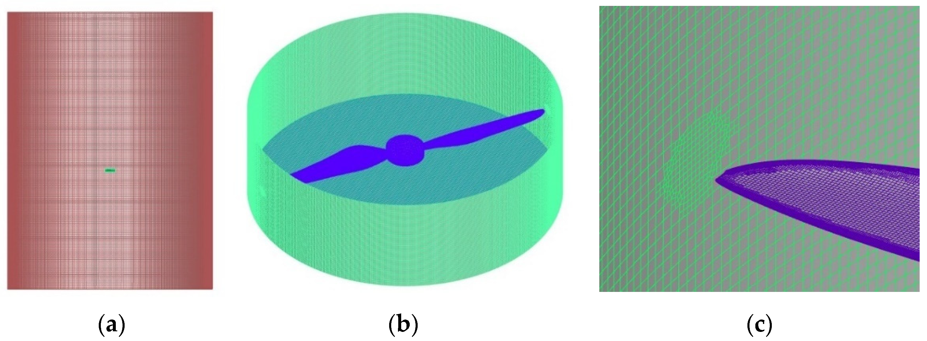
2.3.2. Numerical Simulation Calculations

The current cost of sending UAVs to Mars is considerably expensive, therefore, before proceeding to Mars propeller manufacturing, extensive finite element simulations are required to ensure the dynamics of the propeller system. Since there are difficulties in determining the aerodynamic properties of propellers designed for the Martian environment using purely empirical formulas, Fluent software was used to perform aerodynamic analysis of the Mars propeller. In the numerical simulation, different angles of attack and rotational speeds of the Mars propeller were considered, and the range of angles of attack was taken from 0° to 12°, being calculated every 2° (the results were only taken from 0° to 10° due to the poor convergence of the calculation results at 12° angle of attack). Meanwhile, the range of rotational speeds could be roughly derived from the speed of sound and Mach number of the Martian atmosphere. The range of rotational speeds can be calculated using Equation (20):

$$n<\frac{Ma*a*60}{D*\pi }$$

(20)

where n is the rotational speed in RPM (Revolutions Per Minute); $Ma$ is the Mach number, which is taken as 0.85 to avoid transonic effects; $a$ is the speed of sound in the Martian atmosphere, which is taken as 230 $\mathrm{m}/\mathrm{s}$; and D is the propeller diameter, which is taken as 1.21 m. The maximum rotational speed of the designed Mars propeller was calculated to be 3087 RPM. Because the air density on Mars is low, when the speed is small, the lift provided by the propeller is small; therefore, the simulated speed was selected as 1200 RPM to 3000 RPM, being calculated every 200 RPM.

In order to simulate the Martian atmosphere as much as possible, the atmospheric density was set to the atmospheric density of Mars (0.0167 kg/m³). Figure 6 shows the scheme of the whole computational domain. The whole computational domain is divided into a static domain (a) and a rotating domain (b). These two domains are connected by three pairs of interfaces, namely interface-prop-up and interface-far-up, interface-prop-down and interface-far-down, and interface-prop-wall and interface-far-wall. The static domain is a cylinder with a diameter of 20D and a height of 15D, which is used to simulate the outflow field of the Martian propeller. Figure 6c shows the mesh details of the propeller surface and the blade tip near the wall of the rotating domain. It can be seen that the leading and trailing edges of the propeller and the tip of the blade near the rotating field have a more dense grid, which is done to have more accurate calculation results. Numerical calculations of lift coefficients and power coefficients were performed for the Mars propeller at different angles of attack and rotational speeds, and the results were compared and analyzed with the results obtained from the simulated Mars atmospheric bench experiments in Section 3.2.

In order to investigate the influence of the number of grids on the calculation results, 3 different densities of grids were selected, and then the thrust and torque of the propeller were calculated at a 0° angle of attack and 3000 RPM under the Martian atmosphere. The calculation results are shown in

Table 2. Results of the grid dependency test for prototype.

	Mesh Density (104)	Simulation Time (h)	Thrust Error	Torque Error
Coarse	1237	15	5.77%	6.228%
Medium	2506	26	0.985%	2.076%
Fine	5032	38	0%	0%

.

Numerical simulation analysis was conducted by means of the same method for the aforementioned three grid density models. From the results, an observation can be made that the difference between the results calculated by the medium density grid and the high density grid was considerably small, while the error of the results calculated by the low density grid was relatively large. As such, considering the calculation accuracy and calculation efficiency, the medium density grid was ultimately chosen for the numerical calculation. Figure 7 visualizes the vortex structure of the flow field at a high speed rotation of the propeller with a 0° angle of orientation in the Martian atmospheric environment by extracting the equivalent surface of the Q-criterion = 5000, and also shows the pressure (Unit: Pa) distribution on the propeller blade. It can be seen that as the propeller speed increases, the vortex volume generated at the tip of the propeller blade becomes larger and thicker below the blade, and at the same time, the vortex core increases. The pressure contour diagram shows that the pressure on the propeller blade increases as the speed increases, and the closer the tip, the greater the negative pressure, while the maximum positive pressure is found at the leading edge of the blade near the tip, which is due to the interaction with the air when the propeller rotates at high speed.

2.4. Lightweight Design and Strength Calibration of Mars Propellers

The low air density and low Reynolds number of the Martian atmospheric environment poses a significant challenge in propeller design and fabrication. The low density reduces the available thrust for a given size rotor and increases the power required to fly the vehicle relative to the Earth’s atmospheric environment. Thus, as a critical factor, the overall weight of the vehicle must be kept as low as possible. Obviously, reducing the weight of the propeller is more simple and logical than reducing the weight of the electronics. To ensure optimal performance in the Martian environment, a propeller must possess sufficient lift-to-weight ratio, which necessitates a lightweight design. Consequently, the pursuit of reduced weight has emerged as a significant challenge in the development and production of propellers intended for Mars.

In order to reduce the weight of the propeller, a foam sandwich structure was adopted, with the propeller having foam in the middle and the outside being covered with carbon fiber fabric, as shown in Figure 8a. The yellow part is the PMI (Polymethacrylimide) foam core part, and the gray part is the T300 carbon fiber covered part. The surface area of the whole propeller is 0.098 m², and local reinforcement was performed at the root of the propeller to ensure the strength of the propeller. The density of the fabric prepreg is 1600 kg/m³, the thickness of the single layer is 0.2 mm, and the lay-up direction is 0°/90°/45°. The total weight of a single propeller was calculated to be 100 g when laying 3 layers of carbon fiber fabric.

Although the foam sandwich structure largely reduced the weight of the Mars propeller, the strength and stiffness of the propeller were inevitably weakened while satisfying the lightweight requirements. Thus, the propeller must be calibrated for strength and other aspects before manufacturing. In this study, the HyperMesh and Nastran finite element software were used for joint simulation to check the deformation and failure factor of the propeller. The finite element model of the propeller is shown in Figure 8b.

The aerodynamic force (aerodynamic force at 10° angle of attack, 3000 RPM) obtained from aerodynamic simulation of the propeller under the Martian atmosphere was loaded onto the surface of the propeller, and the deformation of the propeller under the Martian atmosphere (as shown in Figure 9a) and the failure factor of the carbon fiber layup on the surface of the propeller (as shown in Figure 9b) could be obtained. From the deformation diagram, an observation can be made that the main deformation of the propeller was concentrated in the tip part of the propeller blade, and the maximum deformation was 19.8 mm, which was only 3.3% of the radius of the Mars propeller. As such, the stiffness of the propeller meets the requirements. As the trailing edge part of the propeller is considerably thin and is seriously affected by the trailing vortex during high speed rotation, the failure factor of the trailing edge part was also the largest. From the simulation results, the maximum failure factor was 0.11, much less than 1, meaning that the strength of the blade had a large surplus.

2.5. First-Generation Mars UAV Flight

The harsh Martian atmosphere poses a significant challenge in the design of unmanned helicopters, while the spatial size of the lander further limits the size of the Mars UAV. A reasonable structural layout can satisfy the structural size while minimizing the weight of the UAV. The co-axial twin propellers were chosen as the initial structure form for the Mars UAV, as illustrated in Figure 10.

2.5.1. Dynamical Equations and Equations of Motion of an Unmanned Helicopter on Mars

Assuming that the Mars unmanned helicopter is a rigid body, ignoring the Martian curvature, and considering the Martian coordinate system as an inertial coordinate system, the equations of motion of the Mars unmanned helicopter can be divided into two parts to describe the translational and rotational motion, and according to the Newton-Euler equation, the translational motion of the Mars unmanned helicopter can be expressed as:

$$\dot{\mathit{V}}=\frac{\mathit{F}}{{\mathit{m}}_{\mathit{b}}}-{\mathit{\omega }}_{\mathit{b}}\times {\mathit{V}}_{\mathit{b}}$$

(21)

$${\dot{\mathit{\omega }}}_{\mathit{b}}={\mathit{I}}^{-1}[\mathit{M}-{\mathit{\omega }}_{\mathit{b}}\times \left(\mathit{I}{\mathit{\omega }}_{\mathit{b}}\right)]$$

(22)

where $m_b$ indicates the total mass of the Mars unmanned helicopter; ${\mathit{V}}_{\mathit{b}}={\left(\mathit{u},\mathit{v},\mathit{w}\right)}^{\mathit{T}}$ represents the linear velocity of the Mars unmanned helicopter; ${\mathit{\omega }}_{\mathit{b}}={\left(\mathit{p},\mathit{q},\mathit{r}\right)}^{\mathit{T}}$ represents the angular velocity of the Mars unmanned helicopter; $\mathit{F}$ and $\mathit{M}$ represent the combined external force and moment of the Mars unmanned helicopter; and $I$ indicates the moment of inertia of the Mars unmanned helicopter.

$$\mathit{I}=\left(\begin{array}{l}\begin{array}{ccc}{I}_{xx}& -I_{xy}& -I_{xz}\end{array}\\ \begin{array}{ccc}-I_{xy}& I_{yy}& -I_{yz}\end{array}\\ \begin{array}{ccc}-I_{xz}& -I_{yz}& I_{zz}\end{array}\end{array}\right)$$

(23)

Due to the peculiarities of the Martian unmanned helicopter in structure, the belief of the present authors is that the symmetry in both the transverse plane and the longitudinal plane had $I_{xy}=I_{xz}=I_{yz}=0$, and Equation (24) can be converted to:

$$\mathit{I}=\left(\begin{array}{l}\begin{array}{ccc}{I}_{xx}& 0& 0\end{array}\\ \begin{array}{ccc}0& I_{yy}& 0\end{array}\\ \begin{array}{ccc}0& 0& I_{zz}\end{array}\end{array}\right)$$

(24)

By bringing the linear velocity, angular velocity, and resultant force of the three axes of the Mars unmanned helicopter into Equation (21), the linear motion equation of the Mars unmanned helicopter can be obtained:

$$\begin{array}{l}m\left(\frac{du}{dt}+wq-vr\right)+mg\sin \theta =X\\ m\left(\frac{dv}{dt}+ur-wp\right)+mg\cos \theta \cos \varphi =Y\\ m\left(\frac{dw}{dt}+vp-uq\right)-mg\cos \theta \sin \varphi =Z\end{array}$$

(25)

where $u$, $v$, $w$ are the linear velocities along the $O_b{X}_b,O_b{Y}_b,O_b{Z}_b$ axes, respectively; $p,q,r$ are the angular velocities around the $O_b{X}_b,O_b{Y}_b,O_b{Z}_b$ axes, respectively; $X,Y,Z$ are the net forces acting on the $O_b{X}_b,O_b{Y}_b,O_b{Z}_b$ axes, respectively.

The velocity differential equation can be obtained by sorting out Equation (26):

$$\left[\begin{array}{l}\dot{u}\\ \dot{v}\\ \dot{w}\end{array}\right]=\frac{1}{m_b}\left[\begin{array}{l}X\\ Y\\ Z\end{array}\right]+\left[\begin{array}{l}-g\sin \theta \\ g\cos \theta \sin \varphi \\ g\cos \theta \cos \varphi \end{array}\right]+\left[\begin{array}{ccc}0& -r& q\\ -r& 0& -p\\ -q& p& 0\end{array}\right]\left[\begin{array}{l}u\\ v\\ w\end{array}\right]$$

(26)

The linear velocity, angular velocity, and moment of inertia of the three axes of the Mars unmanned helicopter were brought into Equation (22) to obtain the angular motion equation of the UAV around the center of mass:

$$\begin{array}{l}{I}_x\frac{dp}{dt}+\left(I_z-I_y\right)qr=L\\ I_y\frac{dq}{dt}+\left(I_x-I_z\right)pr=M\\ I_z\frac{dr}{dt}+\left(I_y-I_x\right)pq=N\end{array}$$

(27)

where $I_x,I_y,I_z$ are, respectively, the rotational inertia of the unmanned helicopter on the $O_b{X}_b,O_b{Y}_b,O_b{Z}_b$ axes, respectively; $L,M,N$ are the sum of the torques rotating about the $O_b{X}_b,O_b{Y}_b,O_b{Z}_b$ axes, respectively.

According to Equation (27), the angular rate differential equation can be calculated using Equation (28):

$$\left[\begin{array}{l}\dot{p}\\ \dot{q}\\ \dot{r}\end{array}\right]=I^{-1}\left(\left[\begin{array}{l}L\\ M\\ N\end{array}\right]-\left[\begin{array}{ccc}0& -r& q\\ r& 0& -p\\ -q& p& 0\end{array}\right]\times I\left[\begin{array}{l}p\\ q\\ r\end{array}\right]\right)$$

(28)

According to the relationship between attitude angle and angular rate, the rotation kinematics equation can be written as follows:

$$\left[\begin{array}{l}\dot{\varphi }\\ \dot{\theta }\\ \dot{\psi }\end{array}\right]=\left[\begin{array}{ccc}1& \sin \varphi \tan \theta & \cos \varphi \tan \theta \\ 0& \cos \varphi & \sin \varphi \\ 0& \sin \varphi \sec \theta & \cos \varphi \sec \theta \end{array}\right]\left[\begin{array}{l}p\\ q\\ r\end{array}\right]$$

(29)

2.5.2. System Nonlinear Model

For Mars unmanned helicopters, the lift thrust moment on the $O_b{Z}_b$ axis is provided by the reverse torque of the upper and lower propellers—that is, $N=N_T=-N_{D1}+N_{D2}$—and the torque on the $O_b{X}_b$ axis and $O_b{Y}_b$ axis is mainly provided by the servos—that is, $L=L_T,M=M_T$. Assuming that the angular velocity of the upper and lower rotors is ${\Omega }_1,{\Omega }_2$, the thrust generated by the upper and lower rotors can be expressed as:

$$\begin{array}{l}{F}_1=b{\Omega }_1^2\\ F_2=b{\Omega }_2^2\end{array}$$

(30)

where b is the thrust coefficient. The motion characteristics of the Mars unmanned helicopter in the previous section could be sorted out and simplified, because the test flight was mainly aimed at simulating the vacuum chamber environment of the Martian atmosphere, ignoring external interference, such as strong winds. When hovering in a vacuum chamber, the air resistance is relatively small and, therefore, negligible, resulting in a simplified mathematical model:

$$\{\begin{array}{l}\ddot{x}=\dot{u}=\left(\sin \theta \cos \varphi \cos \psi +\sin \varphi \sin \psi \right)\frac{b\left({\Omega }_1^2+{\Omega }_2^2\right)}{m}\\ \ddot{y}=\dot{v}=\left(\sin \theta \cos \varphi \cos \psi -\sin \varphi \cos \psi \right)\frac{b\left({\Omega }_1^2+{\Omega }_2^2\right)}{m}\\ \ddot{z}=\dot{w}=\cos \varphi \cos \theta \frac{b\left({\Omega }_1^2+{\Omega }_2^2\right)}{m}-g\\ \ddot{\varphi }=\frac{\left(I_y-I_z\right)}{I_x}\dot{\theta }\dot{\psi }+\frac{L}{I_x}\\ \ddot{\theta }=\frac{\left(I_z-I_x\right)}{I_y}\dot{\varphi }\dot{\psi }+\frac{M}{I_y}\\ \ddot{\psi }=\frac{\left(I_x-I_y\right)}{I_z}\dot{\varphi }\dot{\theta }+\frac{N}{I_z}\end{array}$$

(31)

3. Results

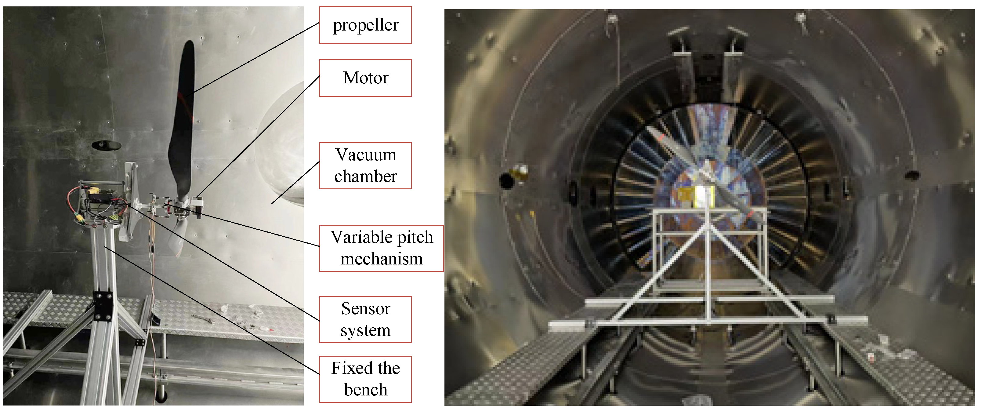
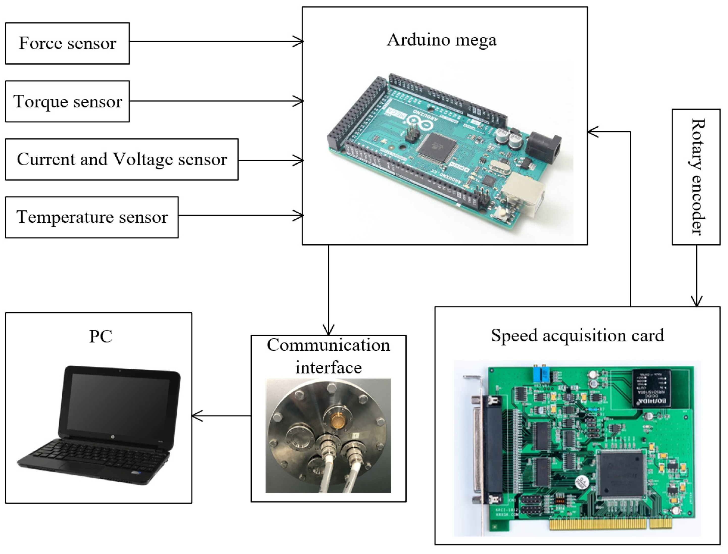
3.1. Experimental Protocol

Due to the large differences between the Martian environment and the Earth environment, the designed propeller needed to be further verified experimentally, and the Martian atmospheric environment needed to be restored as much as possible during the experiment. In the hovering experiments, the UAV hovering performance test device was used to measure the aerodynamic parameters of the Mars rotor system simulating the Martian atmospheric environment, and the feasibility of UAV flight in the Martian environment was evaluated. Such methods can verify the rationality of the model of the simulation method, intuitively reflect the dynamic performance of the UAV, and realize the evaluation of the aerodynamic characteristics of the rotor system of the Mars UAV. The experiment was conducted at the Vacuum Chamber Experimental Base of the China Academy of Aerospace, as illustrated in Figure 11. The chamber has a diameter of 4 m and a depth of 10 m, and can maintain a pressure below 10 Pa. However, notably, the experiment could not entirely replicate the Martian environment. The atmospheric density could only be reduced to approximate that of the Martian atmosphere. The temperature and gravitational acceleration could not simulate the Martian atmospheric environment. Additionally, due to the limitations of the experimental conditions, the composition of the atmosphere could not be the same as that of Mars.

During the experiment, the propeller test bench was placed in a vacuum chamber for fixation, and then the air density in the vacuum chamber was reduced to be comparable to the density of air on Mars. The test bench was designed according to the size of the interface in the vacuum chamber. In order to reduce the wall effect, the diameter of the propeller disc was parallel to the diameter of the vacuum chamber when designing the bench, and at the same time, the propeller was placed 4 m away from the outlet during installation, so as to reserve as much space as possible for the tail and minimize flow recirculation. During the experiment, a T-Motor MN7005 brushless motor was used, which could increase the speed of the propeller to 3000 RPM at the density of the Martian atmosphere, reaching the subcritical acoustic velocity. The test bench of the propeller in the vacuum chamber was installed, as shown in Figure 12, and the propeller retention frame was connected to the aisles on both sides of the cabin to fix the entire test bench. The main performance parameters of each sensor on the test bench are shown in

Table 3. Main performance parameters of each sensor.

	Range	Accuracy
Force sensor/kg	0~3	0.2% ± 20 g
Temperature sensor/°C	−40~350	±1% ± 1.5
Voltage sensor/V	11~55	±0.03% ± 0.03
Current sensor/A	0.2~80	±0.4% ± 0.1
Speed sensor/rpm	1500~3000	±0.5% ± 20

. Under conditions of air density equivalent to that of the Martian atmosphere, the propeller generated a relatively small pull force at a low speed. As a result, the measured value of the pull force at a low speed was not significantly high. Additionally, due to the limited accuracy of the thrust sensor, the thrust error measured at a low speed was relatively large. Therefore, the final rotation speed range of 1200 RPM to 3000 RPM was chosen to measure the pull and torque of the propeller.

Figure 13 shows a schematic diagram of the data acquisition system. The force sensor, torque sensor, temperature sensor, current and voltage sensor are connected to the Arduino mega development board. The pulse signal output by the rotary encoder is also transmitted to the Arduino mega development board through the speed acquisition card, and then communicated with the personal computer through the serial port and the information interaction port on the vacuum bin.

During the experiment, the propeller was subjected to thrust and torque tests at different speeds and different angles of attack. The rotation speed range was 1200 RPM to 3000 RPM, being measured every 200 RPM, and the angle of attack was 0° to 10°, being measured every 2°. The reason for the angle of attack only being 10° is that when using commercial software CFD for aerodynamic simulation, the convergence of the calculation results was not good when the angle of attack was greater than 10°, and the aerodynamic performance of the propeller was reduced. Such findings could be attributed to the fact that with the increase in the angle of attack, laminar flow separation occurs on the surface of the blade, thereby reducing the aerodynamic efficiency of the propeller. During the experiment, the pitch mechanism could be used to change the angle of attack of the propeller, thereby significantly saving costs and avoiding uneven air density in the vacuum chamber after each air extraction caused by multiple openings. Each set of data was measured four times, and then the average data were obtained by adopting the average method.

3.2. Experimental Results and Analysis

The lift thrust coefficient is the main parameter for characterizing the thrust characteristics of propellers, and the data obtained by the vacuum chamber bench test simulating the Martian atmospheric environment were compared with the data calculated by CFD numerical simulation. The results measured by the experiment obviously have the same trend as the results obtained by the CFD simulation, but there were certain errors between the two.

The difference in rotational speed caused the Reynolds number on the surface of the blade to change, which affected the thrust coefficient. As shown in Figure 14, as the rotational speed increases, the thrust coefficient would also slowly increase. However, the changes observed were notably not significant, and the thrust coefficient of the propeller demonstrated nearly identical changes with speeds at different angles of attack. The experimental results indicate that the thrust coefficient of the propeller exhibited varying changes at different angles of attack, and on average, the magnitude of the changes observed was greater than those shown by numerical simulation results.

Undoubtedly, the angle of attack has the most significant influence on the thrust coefficient. In general, as the angle of attack increases, the thrust coefficient also increases. However, when the angle of attack exceeds a certain threshold, the laminar flow over the surface of the propeller separates, resulting in a reduction of the thrust coefficient. Therefore, changes in the angle of attack should be within a reasonable range. During the CFD numerical simulation of the propeller, the convergence effect of the thrust coefficient calculation was found to deteriorate significantly when the angle of attack exceeded 10°. Therefore, the aerodynamic performance of the propeller was analyzed only in the range of angle of attack between 0° and 10°. The CFD numerical simulation results show that with the increase in the angle of attack, the thrust coefficient almost increased in the form of an equal difference series, and the maximum thrust coefficient was achieved when the angle of attack was 10° and the speed was 3000 RPM. Compared with the numerical simulation results, the experimental results were more volatile. In the range of 0° to 8°, with the increase in the angle of attack, the thrust coefficient increased, but unlike the CFD simulation results, when the angle of attack was 10°, the thrust coefficient was smaller than the thrust coefficient when the angle of attack is 8°. At the same time, the changes in the thrust coefficient between adjacent angles of attack did not show equal differences compared with the numerical simulation, which was caused by equipment and environmental errors during the test.

The thrust coefficient can be calculated using Equation (32):

$$C_T=\frac{3600T}{\rho n^2{D}^4}$$

(32)

where T is the thrust generated by the propeller during rotation; ρ is the density of the Martian atmosphere; n is the rotational speed of the propeller in the Martian atmospheric environment; and D is the diameter of the paddle disc of the Mars propeller.

The power factor Cp is a performance indicator that measures the efficiency of propellers. The increase in the angle of attack means that the windward area of the propeller when rotating at high speed also increases, the resistance is correspondingly increased, and the power consumed is greater. As shown in Figure 15, comparing the CFD numerical simulation results and the vacuum chamber bench experimental results, an observation can be made that, in respect of numerical terms, the difference between the two was considerably large, and the results measured by the vacuum chamber bench test were obviously much larger than the CFD numerical simulation results; but, in terms of trends, the two were similar. As shown in Figure 15, with the increase in the angle of attack, the difference in the power coefficient between the adjacent angles of attack also increased, and at the same angle of attack, the speed increased, but the power coefficient showed a slight decrease, which is because the larger the rotational speed, the greater the inertia generated when the propeller rotates. In this way, the power loss can be reduced to a certain extent. The experimental data indicate that under the same angle of attack, the power coefficient of the propeller gradually decreases with an increase in speed. Moreover, within the range of 0° to 8° blade angles, the power coefficient increased with the angle of attack. Additionally, the greater the angle of attack, the more the power coefficient was affected by the increase in rotational speed. Notably, the power coefficient obtained from the experimental test was markedly different from the power coefficient obtained by CFD simulation. Specifically, under the same angle of attack, the power coefficient changed only slightly with an increase in rotational speed in the CFD simulation, while the experimental data showed a substantial change in the power coefficient with the increase in rotational speed. The biggest difference still occurred in the case of an angle of attack of 10°, and the experimental data show that when the rotational speed was less than 2400 RPM, the power coefficient at an angle of attack of 10° was significantly smaller than the power coefficient at an angle of attack of 8°. However, when the rotational speed was greater than 2400 RPM, the opposite trend could be seen, and as the rotational speed increased, the power coefficient at an angle of attack of 8° further decreased.

The power factor can be calculated using Equation (33):

$$C_p=\frac{3600P}{\rho n^3{D}^5}$$

(33)

where P is the power consumed by the Martian propeller as it rotates in the Martian atmosphere.

The merit factor is one of the main factors in evaluating the performance of the propeller, and the higher the merit factor, the higher the efficiency of the propeller in such states. The CFD numerical simulation results shown in Figure 16 indicate that, with the increase in propeller angle of attack, the merit factor also increased, but the increase became increasingly smaller. When the angle of attack was 8° and 10°, the merit factor of the propeller was roughly equal. At the same time, with the increase in speed, the merit factor also increased correspondingly; and, under the same angle of attack, the merit factor increases linearly with the increase in speed. There was a significant difference between the merit factor obtained from the vacuum warehouse bench experiment and the CFD numerical simulation. Not only was there a difference in value, but also in trend. The merit factor measured by the vacuum warehouse bench experiment did not increase with the angle of attack, but presented a disorderly pattern. However, the merit factor under the same angle of attack still increased with the increase in speed. At an angle of attack of 8° and a speed of 3000 RPM, the merit factor was optimal. Considering the thrust coefficient and power coefficient, it can be concluded that the optimal performance could be achieved at an angle of attack of 8°.

The merit factor can be calculated using Equation (34):

$$FM=\frac{1}{\sqrt{2}}\frac{C_l^{3/2}}{C_p}$$

(34)

where $C_l$ and $C_p$ indicate the thrust coefficient and power coefficient, respectively.

From the comparison of the experimental data and CFD simulation data, although there were errors therebetween, the general trend was the same. Therefore, to some extent, the CFD simulation results can be used to judge the quality of propeller design. In order to verify whether there was an increase in error caused by the vacuum chamber environment, we attempted to conduct outdoor experiments using the same experimental equipment in a calm environment, and conducted CFD simulations using the same numerical simulation methods. Comparing the numerical results with the simulation results, the errors of the thrust coefficient and torque coefficient are both within 10%. The specific experimental data will be presented in another manuscript. Therefore, we believe that the factor causing significant errors is the significant difference between the vacuum chamber environment and the open environment on Mars. The belief of the present authors is that the following reasons could have caused the errors:

(1)

In the process of pumping the density of air in the vacuum chamber to the same as that of the Martian atmosphere, there were errors, and there were difficulties in achieving exactly the same between the two;

(2)

The accuracy of force and torque sensors was not enough, leading to the deviation of the tested data;

(3)

Due to the mechanism of the experimental bench, a great centrifugal force will be generated when the propeller rotates at a high rotational speed, which will lead to the vibration of the test bench in the process of testing, and then produce a certain deviation;

(4)

Due to the existence of an idle stroke (due to mechanical structural gaps), the angle of attack will produce a certain deviation in each variation of pitch, which will affect the experimental results to a great extent;

(5)

The vacuum chamber is a closed container. In the process of the experiment, certain wall effects and air reflux will be formed.

3.3. Mars Unmanned Helicopter Hover Experiment

The limited space within the vacuum chamber makes it challenging to perform maneuvering flight experiments. Therefore, the primary goal for the original Mars unmanned helicopter was to verify its hovering performance in the vacuum chamber. Notably, the gravitational acceleration on Mars is only one-third of that on Earth, and to simulate the Martian environment, the other two-thirds of Earth’s gravitational acceleration were counterbalanced by lifting heavy objects at one end of the pulley set. As the vacuum chamber equipment was unable to fully simulate the Martian atmospheric environment—with the temperature in the chamber being maintained at Earth’s room temperature—there was a failure to replicate the significantly lower temperature on Mars. In order to ensure that the Mars unmanned helicopter achieved hovering in an environment similar to the Mars air density, the pressure in the vacuum chamber was extracted to a pressure of approximately 1950 Pa instead of the Martian atmospheric pressure of 756 Pa. To achieve control, the hovering of the Mars unmanned helicopter was realized using a PID control, as shown in Figure 17, which illustrates the hovering state of the first generation of a Mars unmanned helicopter in the vacuum chamber simulating the Martian atmospheric environment.

4. Conclusions

In the present study, by analyzing the dynamic conditions of the Martian atmospheric environment, a rotor system suitable for the Martian atmospheric environment was designed and a strength test of the lightweight Martian propeller was conducted by means of the finite element method. At the same time, the aerodynamic characteristics of the Martian propeller in the Martian atmospheric environment were explored by combining numerical simulations and vacuum chamber experiments. The following conclusions could be drawn:

(1)

In order to reduce the weight of the Martian propeller, the adopted foam sandwich structure had a good weight reduction effect, and through finite element calculation and Earth environment bench experiments, the three-layer carbon fiber ply was verified to not only meet the lightweight and strength requirements, but also meet the requirements of the manufacturing process, which is the most suitable manufacturing method of the Mars propeller at present.

(2)

Under the CFD numerical simulation, when the angle of attack was fixed, the thrust coefficient of the Martian propeller increased with the increase in speed, and the power coefficient decreased accordingly. The merit factor also increased with the increase in the propeller speed. When the propeller speed was constant, the thrust coefficient and power coefficient of the propeller increased accordingly with the increase in angle of attack, and the merit factor also increased accordingly. However, at 8° and 10° angles of attack, it had almost the same quality factor.

(3)

A vacuum chamber experiment simulating the Martian atmospheric environment was conducted on the Martian propeller, and the aerodynamic characteristics of the Martian propeller in the Martian atmospheric environment were further explored. There was an error between the experimental results and the numerical simulation results, mainly because the numerical simulation was a simulation calculation in an ideal environment, while the experimental test had many external interferences, but the two exhibited roughly the same trend.

(4)

The numerical simulation method considered the unsteady compressible flow and the vacuum chamber experiment of the simulated Martian atmospheric environment verified that the designed propeller system had good aerodynamic performance in the Martian atmospheric environment. On this basis, the initial design of the Mars unmanned helicopter was formulated, and the relevant hover experiments were conducted, providing reference and theoretical support for the design of subsequent Mars UAV sequences.

References

1. Petritoli, E.; Leccese, F. Unmanned Autogyro for Mars Exploration: A Preliminary Study. Drones 2021, 5, 53. [Google Scholar] [CrossRef]
2. Wu, W.R.; Yu, D.Y. Development of deep space exploration and its future key technologies. J. Deep Space Explor. 2014, 1, 5–17. [Google Scholar]
3. Datta, A.; Roget, B.; Griffiths, D.; Pugliese, G.; Sitaraman, J.; Bao, J.; Liu, L.; Gamard, O. Design of a Martian autonomous rotary-wing vehicle. J. Aircr. 2015, 40, 461–472. [Google Scholar] [CrossRef]
4. Chi, C.; Lumba, R.; Su Jung, Y.; Datta, A. Aeromechanical Analysis of a Next-Generation Mars Helicopter Rotor. J. Aircr. 2022, 59, 1463–1477. [Google Scholar] [CrossRef]
5. Ruiz, M.C.; D’Ambrosio, D. Aerodynamic optimization and analysis of quadrotor blades operating in the Martian atmosphere. Aerosp. Sci. Technol. 2023, 132. [Google Scholar]
6. Balaram, J.; Aung, M.; Golombek, M.P. The Ingenuity Helicopter on the Perseverance Rover. Space Sci. Rev. 2021, 217, 2–11. [Google Scholar] [CrossRef]
7. Balaram, J.; Daubar, I.J.; Bapst, J.; Tzanetos, T. Helicopters on Mars: Compelling Science of Extreme Terrains Enabled by an Aerial Platform. In Proceedings of the 9th International Conference on Mars, Pasadena, CA, USA, 22–25 July 2019; Volume 2089. [Google Scholar]
8. Pipenberg, B.T.; Keennon, M.T.; Langberg, S.A.; Tyler, J.D.; Balaram, J. Development of the Mars Helicopter Rotor System. In Vertical Flight Society Annual Forum and Technology Display, Proceedings of the 75th American Helicopter Society Annual Forum, Philadelphia, PA, USA, 13–16 May 2019; Vertical Flight Society: Fairfax, VA, USA, 2019; Volume 382. [Google Scholar]
9. Takaki, R. Aerodynamic characteristics of NACA4402 in low Reynolds number flows. Jpn. Soc. Aeronaut. Space Sci. 2006, 54, 367–373. [Google Scholar]
10. Shrestha, R.; Benedict, M.; Chopra, I. Hover Performance of a Small-Scale Helicopter Rotor for Flying on Mars. J. Aircr. 2016, 53, 1160–1167. [Google Scholar] [CrossRef]
11. Kurane, K.; Uechi, K.; Takahashi, K.; Fujita, K.; Nagai, H. Aerodynamic Characteristics of Mars Airplane Airfoils with Control Surface in Propeller Slipstream. In Proceedings of the 2018 AIAA Aerospace Sciences Meeting, AIAA-2018-2058, Kissimmee, FL, USA, 8–12 January 2018. [Google Scholar]
12. Pipenberg, B.T.; Keennon, M.; Tyler, J.; Hibbs, B.; Langberg, S.; Balaram, J.; Grip, H.F.; Pempejian, J. Design and Fabrication of the Mars Helicopter Rotor, Airframe, and Landing Gear Systems. In Proceedings of the AIAA Scitech 2019 Forum, AIAA-2019-0620, San Diego, CA, USA, 7–11 January 2019. [Google Scholar]
13. Koning, W.J.; Johnson, W.; Grip, H.F. Improved Mars Helicopter Aerodynamic Rotor Model for Comprehensive Analyses. AIAA J. 2019, 57, 3969–3979. [Google Scholar] [CrossRef] [Green Version]
14. Kunz, P.J. Aerodynamics and Design for Ultra-Low Reynolds Number Flight; Stanford University: Stanford, CA, USA, 2003. [Google Scholar]
15. Liu, Z.; Albertani, R.; Moschetta, J.M.; Thipyopas, C.; Xu, M. Experimental and Computational Evaluation of Small Microcoaxial Rotor in Hover. J. Aircr. 2011, 48, 220–229. [Google Scholar] [CrossRef]
16. Bohorquez, F. Rotor Hover Performance and System Design of an Efficient Coaxial Rotary Wing Micro Air Vehicle; University of Maryland: College Park, MD, USA, 2007. [Google Scholar]
17. Oyama, A.; Fujii, K. Airfoil design optimization for airplane for Mars exploration. In Proceedings of the J-55, the Third China-Japan-Korea Joint Symposium on Optimization of Structual and Mechanical Systems, CJK-OSM3, Kanazawa, Japan, 30 October–2 November 2004; pp. 1–3. [Google Scholar]
18. Koning, W.J.; Romander, E.A.; Johnson, W. Low Reynolds number airfoil evaluation for the Mars helicopter rotor. In Proceedings of the American Helicopter Society 74th Annual Forum, Phoenix, AZ, USA, 14–17 May 2018; pp. 1–17. [Google Scholar]
19. Désert, T.; Jardin, T.; Bézard, H.; Moschetta, J. Numerical predictions of low Reynolds number compressible aerodynamics. Aerosp. Sci. Technol. 2019, 92, 211–223. [Google Scholar] [CrossRef] [Green Version]
20. Braun, R.D.; Wright, H.S.; Croom, M.A.; Levine, J.S.; Spencer, D.A. Design of the ARES Mars Airplane and Mission Architecture. J. Spacecr. Rockets 2006, 43, 1026–1034. [Google Scholar] [CrossRef]
21. Marko, Ž.; Ekmedzic; Aleksandar, B.; Boško, R. Conceptual Design and Flight Envelopes of a Light Aircraft for Mars Atmosphere. Teh. Vjesn. 2018, 25, 375–381. [Google Scholar]
22. Chen, S.T. Lift Drag Characteristics and Experimental Study of Mars Probe Rotor Uav; Harbin Institute of Technology: Harbin, China, 2019; pp. 13–17. [Google Scholar]
23. Desert, T.; Moschetta, J.M.; Bezard, H. Numerical and experimental investigation of an airfoil design for a Martian micro rotorcraft. Int. J. Micro Air Veh. 2018, 10, 262–272. [Google Scholar] [CrossRef]
24. Jung, J.; Yee, K.; Misaka, T.; Jeong, S. Low Reynolds Number Airfoil Design for a Mars Exploration Airplane Using a Transition Mode. Jpn. Soc. Aeronaut. Space Sci. 2017, 60, 333–340. [Google Scholar]
25. Mcmasters, J.H.; Henderson, M.L. Low-Speed Single-Element Airfoil Synthesis. Tech. Soar. 1979, 6, 19–23. [Google Scholar]
26. Drela, M. Transonic low-Reynolds number airfoils. J. Aircr. 1992, 29, 1106–1113. [Google Scholar] [CrossRef]
27. Anyoji, M.; Numata, D.; Nagai, H.; Asai, K. Effects of Mach Number and Specific Heat Ratio on Low-Reynolds-Number Airfoil Flows. AIAA J. 2014, 53, 1640–1654. [Google Scholar] [CrossRef]
28. Ananda, G.K.; Sukumar, P.P.; Selig, M.S. Measured aerodynamic characteristics of wings at low Reynolds numbers. Aerosp. Sci. Technol. 2015, 42, 392–406. [Google Scholar] [CrossRef]
29. Okamoto, M. An Experimental Study in Aerodynamic Characteristics of Steady and Unsteady Airfoils at Low Reynolds Number; Nihon University: Tokyo, Japan, 2005. [Google Scholar]
30. Bézard, H.; Désert, T.; Jardin, T.; Moschetta, J.M. Numerical and Experimental Aerodynamic Investigation of a Micro-UAV for Flying on Mars. In Proceedings of the 76th Annual Forum & Technology Display, Online, 5–8 October 2020; Volume 17. [Google Scholar]
31. Liu, P.Q. Theory and Application of Air Propeller; Beijing University of Aeronautics and Astronautics Press: Beijing, China, 2006; pp. 148–234. [Google Scholar]
32. Zahra, S.; Hwang, Y.; Sotoudeh, Z. A Variational Principle for Unsteady Compressible Flow. In Proceedings of the 54th AIAA Aerospace Sciences Meeting, San Diego, CA, USA, 4–8 January 2016; pp. 4–8. [Google Scholar]
Figure 1. General Mach–Reynolds number research areas.
Drones 07 00397 g001
Figure 2. Maximum section lift-to-drag ratio versus Reynolds number.
Drones 07 00397 g002
Figure 3. Force analysis of blade element.
Drones 07 00397 g003
Figure 4. Torsion angle and chord length distribution of different parts of propeller: (a) twist angle distribution; (b) chord length distribution.
Drones 07 00397 g004
Figure 5. Propeller model.
Drones 07 00397 g005
Figure 6. Mars propeller three-dimensional mesh: (a) static zone; (b) rotating zone; (c) blade tip area mesh.
Drones 07 00397 g006
Figure 7. Diagram of propeller vorticity structure on the iso−surface of the Q−criterion = 5000 in Martian: (a) 2000 RPM; (b) 2400 RPM; (c) 2600 RPM; (d) 3000 RPM.
Drones 07 00397 g007
Figure 8. Propeller structure and the finite element model: (a) structure diagram of the foam sandwich of the Mars propeller; (b) finite element model of the Mars propeller.
Drones 07 00397 g008
Figure 9. Finite element analysis results of Mars Propeller: (a) axial direction deformation of the Mars propeller; (b) failure factors of the Mars propeller.
Drones 07 00397 g009
Figure 10. Mars unmanned helicopter model.
Drones 07 00397 g010
Figure 11. A vacuum chamber simulating the atmospheric environment of Mars.
Drones 07 00397 g011
Figure 12. The test system of the Mars propeller in the vacuum chamber.
Drones 07 00397 g012
Figure 13. Data collection system of the test bench.
Drones 07 00397 g013
Figure 14. Thrust coefficient at different rotating speeds and angles of attack.
Drones 07 00397 g014
Figure 15. Power coefficient at different speeds and angles of attack.
Drones 07 00397 g015
Figure 16. Merit factors at different speeds and angles of attack.
Drones 07 00397 g016
Figure 17. Hovering experiment of mars unmanned helicopter in vacuum chamber.
Drones 07 00397 g017