Abstract
Accurate obstacle detection plays a crucial role in the creation of high-precision maps within unstructured terrain environments, as it supplies vital decision-making information for unmanned engineering vehicles. Existing works primarily focus on the semantic segmentation of terrain environments, overlooking the safety aspect of vehicle driving. This paper presents a hazardous obstacle detection framework in addition to driving safety-assured semantic information in the generated high-precision map of unstructured scenarios. The framework encompasses the following key steps. Firstly, a continuous terrain point cloud model is obtained, and a pre-processing algorithm is designed to filter noise and fill holes in the point cloud dataset. The Sobel-G operator is then utilized to establish a digital gradient model, facilitating the labeling of hazardous obstacles. Secondly, a bidirectional long short-term memory (Bi-LSTM) neural network is trained on obstacle categories. Finally, by considering the geometric driving state of the vehicle, obstacles that pose safety risks to the vehicle are accurately extracted. The proposed algorithm is validated through experiments conducted on existing datasets as well as real, unstructured terrain point clouds reconstructed by drones. The experimental results affirm the accuracy and feasibility of the proposed algorithm for obstacle information extraction in unstructured scenes.
1. Introduction
Autonomous engineering vehicles have demonstrated significant potential in various industries, including construction, mining, agriculture, and forestry [1,2]. A fundamental aspect of autonomous driving systems is the utilization of High-Definition (HD) maps, which incorporate semantic information to ensure safe and effective navigation. Semantic maps encompass both geometric mapping and semantic data, playing a crucial role in path planning and navigation tasks [3,4]. In the context of structured road environments, HD maps are generated by collecting point cloud data and images using advanced onboard sensors. These maps contain valuable prior information about complex road conditions, such as road elements, lane lines, traffic signs, and objects of interest [5]. While semantic map construction techniques have been widely employed in urban road scenarios, unstructured environments in which engineering vehicles operate and are characterized by irregular terrain patterns pose distinct challenges. In such environments, clear road boundaries and traffic signs are often absent, and the semantic environment is represented by labeled obstacles and access areas. As a result, the accuracy of semantic segmentation in complex domains significantly deteriorates. Additionally, the harsh vibration and dust present in these environments severely affect the precision and reliability of onboard sensors. Consequently, developing reliable semantic maps for unstructured terrain environments, specifically for autonomous engineering vehicles, becomes even more challenging.
The methods employed for mapping unstructured terrain can be broadly categorized as online real-time scanning and offline data modeling. Real-time terrain scanning, utilizing LiDAR or visual approaches, is a crucial component of Simultaneous Localization and Mapping (SLAM) technology, widely adopted in mobile robotics. For instance, Ebadi et al. implemented and tested a LiDAR-based multi-robot SLAM system for large-scale autonomous mapping in subterranean environments with degraded perception [6]. Pan et al. proposed an online elevation mapping system that rapidly generates dense local elevation maps for fast, responsive local planning while maintaining a globally consistent, dense map for path routing [7]. In comparison to LiDAR mapping, visual modeling facilitates data acquisition and online postprocessing, showcasing its superiority in small-sized field robots and planetary exploration. Matthies et al. discussed the progress in computer vision techniques for planetary rovers and landers, where visual terrain maps provide reliable environmental information for navigation planning and motion control of Mars rovers [8,9]. Ma et al. achieved autonomous 24 hour operation of a dynamic quadruped in complex field terrains through a combination of stereo cameras, an IMU, and leg odometry [10]. Bernuy et al. designed an outdoor semantic mapping method based on visual information and topological maps, enriching the off-road scene with semantic descriptions [11]. Sock et al. estimated the traversability of unstructured terrains and built a probabilistic grid map online using 3D LiDAR and cameras, exploiting the complementary nature of LiDAR and camera data [12].
Real-time terrain modeling aims to achieve efficient data acquisition and mapping in dynamic environments, whereas offline data modeling primarily emphasizes mapping accuracy, particularly for centimeter-scale global maps. Large-scale terrain data is typically collected through manual measurements, LiDAR scanning, and UAV tilt photography. Manual surveying and mapping involve the use of GPS, theodolite, and rangefinder but are mostly suitable for simple, structured scenes due to the manual measurement requirement [13,14]. High-precision LiDAR mapping relies on vehicle or UAV platforms to perform continuous scanning and registration of terrain point clouds, although its high cost restricts its application in autonomous driving systems [15,16,17]. UAV tilt photography, utilizing high-precision cameras, enables the rapid capture of a large number of multi-view images along a designated route. Through camera calibration, matching, and triangulation of image datasets, a 3D terrain model can be generated. This approach offers the comprehensive advantages of low cost, fast modeling, and high accuracy in large-scale, complex outdoor environments [18,19]. Liu et al. produced a high-precision true digital orthophoto map of buildings based on UAV images, validating its accuracy using randomly distributed checkpoints [20]. Liu et al. achieved accurate mapping in UAV photogrammetry without ground control points in the map projection frame, demonstrating elevation accuracy in unstructured terrain environments [21].
While urban road vehicles experience driving instability primarily due to high-speed dynamic operations, lower-speed engineering vehicles in off-road scenarios are more prone to unsafe rollover accidents due to variable vehicle structures and complex terrain environments. This risk is particularly significant when facing occluded visual fields or inaccurate traversability estimation [22,23,24]. Effectively predicting and estimating the risk motion state through a coupled vehicle-terrain dynamic model in unstructured environments enables early risk warning and motion trajectory planning for autonomous engineering vehicles [25]. However, real-time solutions of the coupled model increase the burden on the vehicle control unit and do not provide sufficient time margin for control decision-making in autonomous engineering vehicles. Therefore, integrating safety-assured semantic information into global maps can efficiently provide real-time risk motion states, enabling safe driving operations for off-road engineering vehicles.
In summary, the existing unstructured scenarios predominantly delineate three principal classifications. These classifications encompass natural landscapes inclusive of mountainous terrain and grassland expanses, urban thoroughfares encompassing thoroughfares, architectural constructs, and pedestrian domains, and interior environments characterized by unstructured layouts, furnishings, and ornamental embellishments. Most existing work focuses on semantic segmentation of the terrain environment without considering vehicle dynamics, classifying obstacles of interest as pits, bulges, stones, etc. [26,27]. Additionally, most of the ways to process data require extremely high computational power and deep network structures. This paper proposes a hazardous obstacle detection framework tailored for unmanned engineering vehicles engaged in operations within natural landscapes. The key novelty of this work is the combination of point cloud segmentation techniques with vehicle geometry models. The pre-processing and Bi-LSTM networks employed achieve competitive results without excessive computational power. Furthermore, it provides more effective driving safety semantic information for high-precision maps of unstructured scenes. The main contributions of this paper can be summarized as follows:
- Point cloud filtering algorithms that employ geometric and color spaces to filter outliers and refine unstructured scene point cloud models;
- Introducing the Sobel-G operator to build a digital gradient model. The reverse hole-filling method is designed to address point cloud model defects, and the OTSU segmentation algorithm is employed for further marking of hazardous obstacles;
- Innovative application of a bidirectional long short-term memory (Bi-LSTM) neural network to train point cloud features, facilitating faster and more accurate semantic segmentation of hazardous obstacles in similar unstructured environments;
- Accurate extraction of hazardous obstacles that impact the safe driving of vehicles by leveraging the vehicle-terrain model.
2. Methods
The proposed method is illustrated in Figure 1 and consists of three main stages: pre-processing, deep learning semantic segmentation, and obstacle detection based on the vehicle’s geometric model. The aim is to identify perilous impediments affecting the secure mobility of engineering vehicles and subsequently integrate this data into a high-precision map representation. The hazardous impediments, as posited within this research, specifically refer to convex obstacles encountered within unstructured roadway contexts. In the pre-processing stage, the image point cloud map model undergoes filtering and hole-filling to address the interference caused by outlier points in the point cloud model. Segmentation and filling algorithms are then applied to segment and label the obstacles, providing training data for the deep learning network. Subsequently, the deep learning network quickly extracts obstacles of the same type from the point cloud. Finally, hazardous obstacles that affect the vehicle’s safe driving are segmented in conjunction with the vehicle’s geometric model.
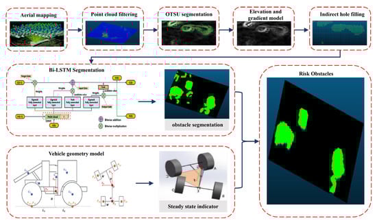
Figure 1.
The framework of hazardous obstacle detection.
2.1. Experimental Equipment and Site
Terrain-based 3D point clouds play a pivotal role in extracting semantic representations. To ascertain the viability of the suggested approach, we utilize UAV tilt photogrammetry for the generation of an image point cloud model dataset specifically tailored for unstructured terrain settings. As depicted in Figure 2, an irregular topographic region spanning an approximate area of 2000 square meters is chosen as the designated site for surveying and modeling endeavors. The planning of aerial routes encompasses five distinct operational directions: a singular orthophoto route and four tilt photography routes directed towards the east, south, west, and north orientations. A comprehensive summary of the key parameters associated with the UAV employed for the experimental activities is furnished in Table 1.
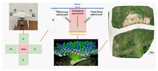
Figure 2.
Experimental equipment and site.

Table 1.
UAV basic parameters.
2.2. Terrain Point Cloud Filtering and Hole Completion
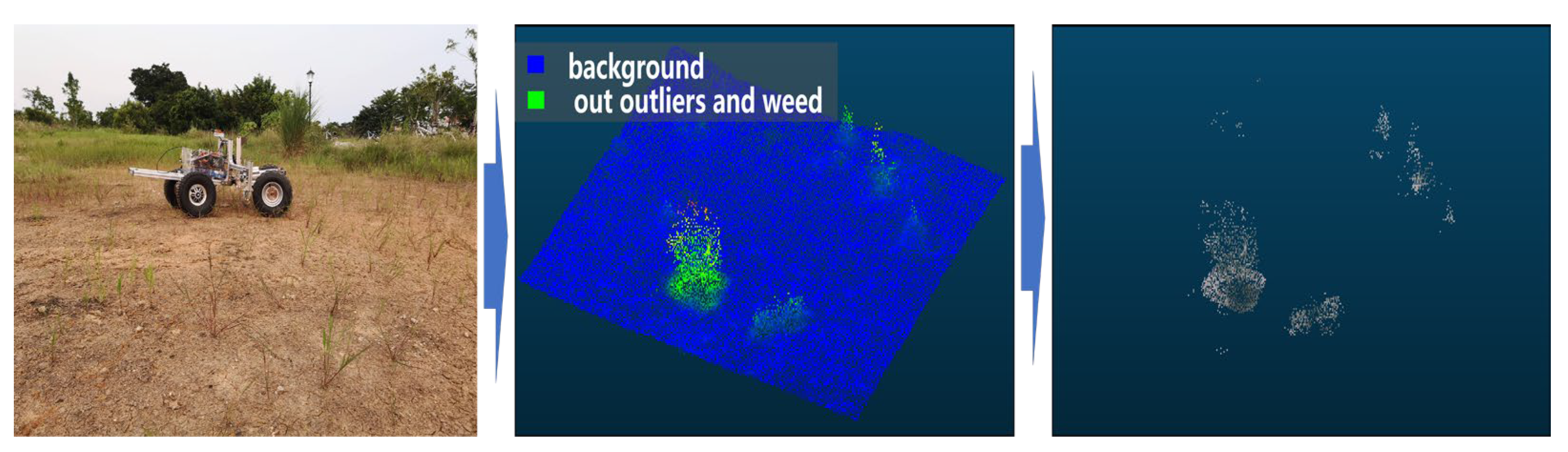
Throughout the image acquisition procedure, the terrain-derived point cloud sourced from the drone’s tilting maneuver often exhibits instances of noise, outliers, and perturbations stemming from carrier frame oscillations, as well as effects introduced by factors like smoke, dust shading, and variations in illumination. Moreover, as illustrated in Figure 3, the presence of weeds within the unstructured environment might not directly compromise the operational security of unmanned engineering vehicles. Nevertheless, these elements can be erroneously interpreted as obstacles within the point cloud data, thereby impinging upon the decision-making process. To faithfully represent the underlying topographical contours, the original point cloud undergoes a preliminary pre-processing stage rooted in statistical filtering, encompassing both geometric and color space domains. This procedural facet encompasses the exclusion of outliers and weed-associated point clouds.
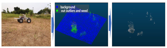
Figure 3.
Unstructured scenario impact factors.
- Geostatistical filtering on outliers
Assuming that the average geometric distance between any point in the point cloud and the surrounding points follows a normal distribution , a filtering threshold of is adopted in this paper. Points with an average distance greater than the threshold are considered outliers and filtered out.
First, the average distance between points in the neighborhood space is calculated using the following formula:
where represents any point in the point cloud, represents a point within the range of point P, and N is the number of points in the neighborhood. The larger the value of , the further the point is from its surrounding points.
A field window of 0.04 square meters has been selected for this paper. Therefore, point K satisfies the following condition:
After that, the expectation (mean) and standard deviation of the point distances from the mean value in the neighborhood space are calculated for all points using the following formulas:
where NUM is the total number of points in the point cloud.
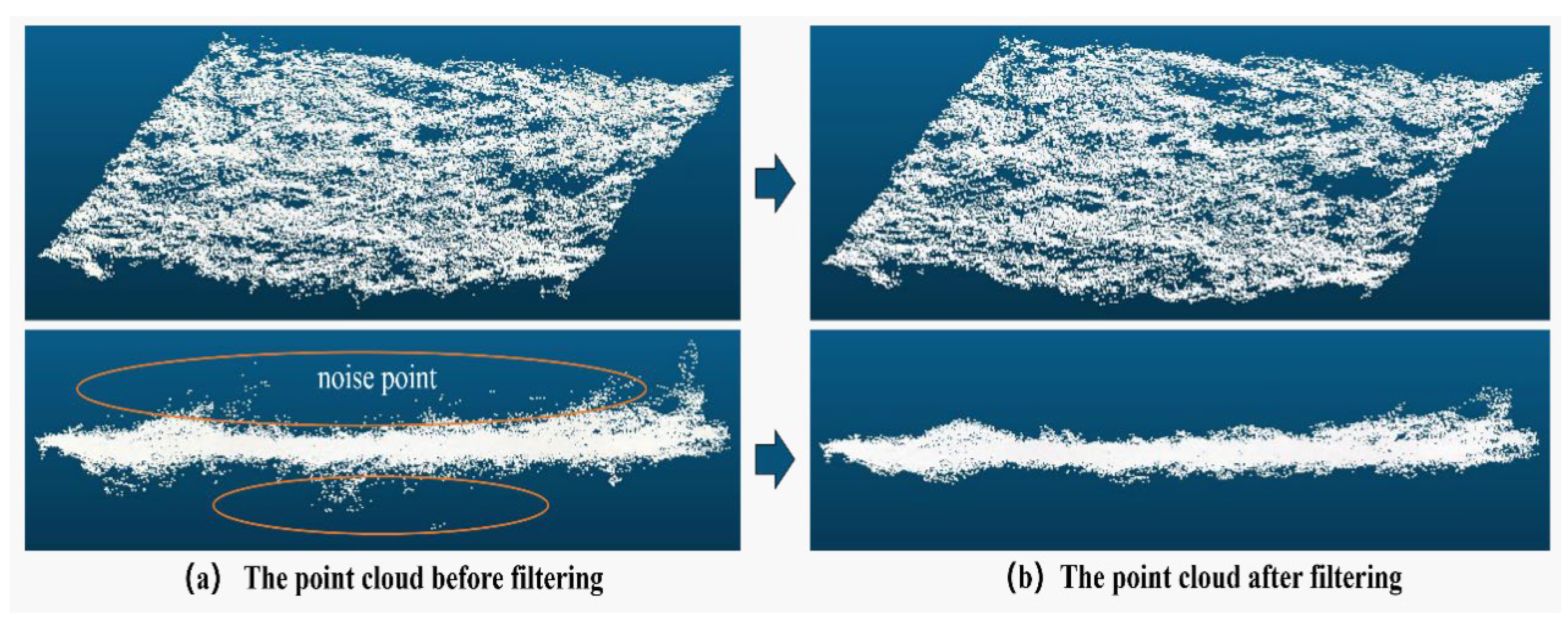
Figure 4 illustrates the effect of the geostatistical filtering algorithm on a group of original terrain point cloud data in a area. The original point cloud data consists of 36,686 spatial point coordinates. After applying the statistical filtering with the filtering threshold set to , the point cloud data is reduced to 33,147 points. The statistical filtering algorithm effectively removes noise and outlier data points, as demonstrated in the figure.
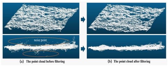
Figure 4.
Comparison before and after statistical filtering.
- Color space statistical filtering on surface weed
Given the inclusion of comprehensive color characteristics within point cloud models derived from unmanned aerial photography and the notable dissimilarity in feature information between weeds and other entities within unstructured terrains, this study presents a method for weed surface filtration utilizing color space statistical filtering.
The point cloud is segmented using a statistical method where the average distance of the RGB color space of neighboring points is used as the evaluation metric. The formula for calculating is as follows:
in the formula, R, G, and B represent the coordinates of the three axes in the RGB color space; are the color space coordinates corresponding to any point in the point cloud; and are the color space coordinates corresponding to point in the neighborhood of point P. N is the number of points in the neighborhood.
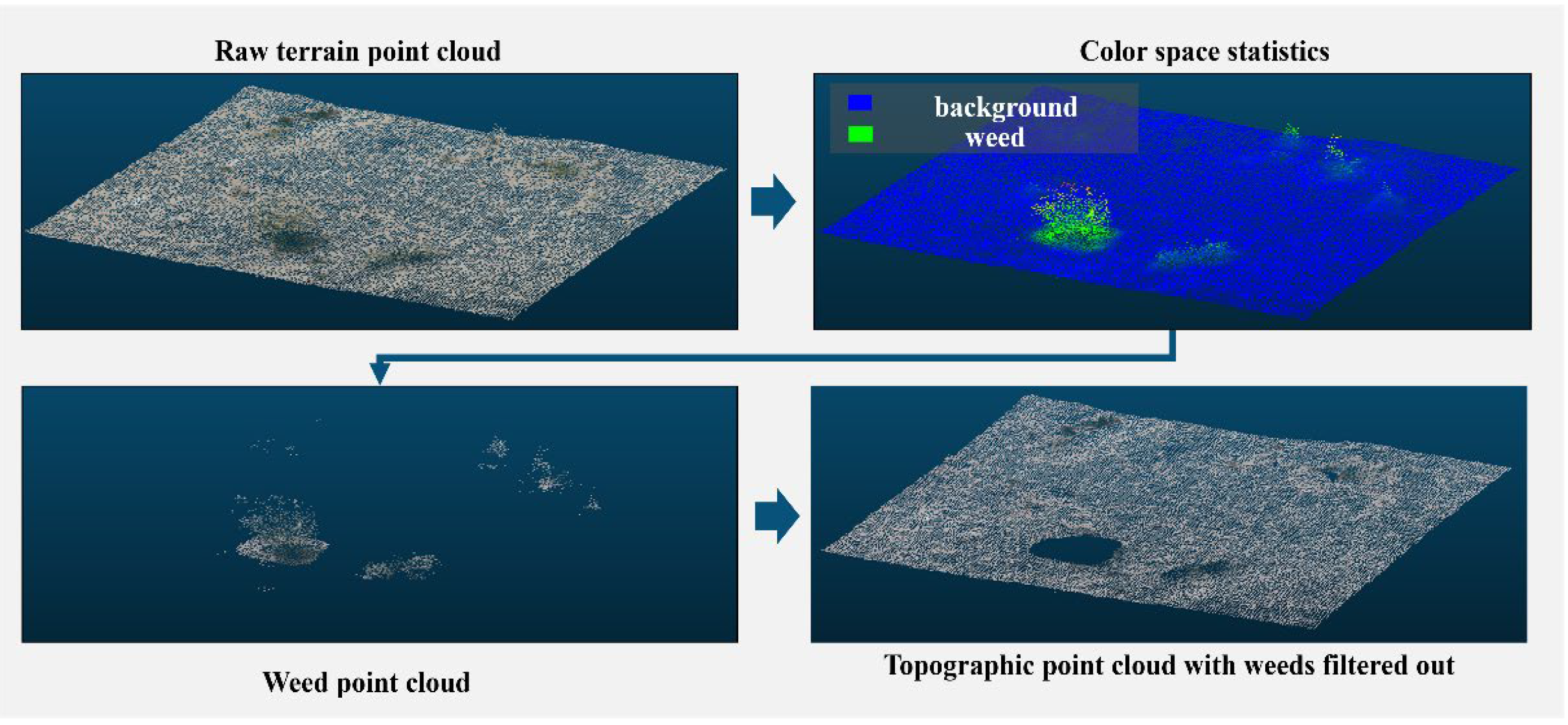
Figure 5 illustrates the effect of color space statistical filtering using the filtering threshold The filtering algorithm described in this paper effectively extracts and separates the surface weed point cloud.
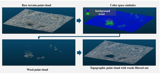
Figure 5.
Color space statistical filtering for weed removal.
- Hole-filling of filtered point clouds
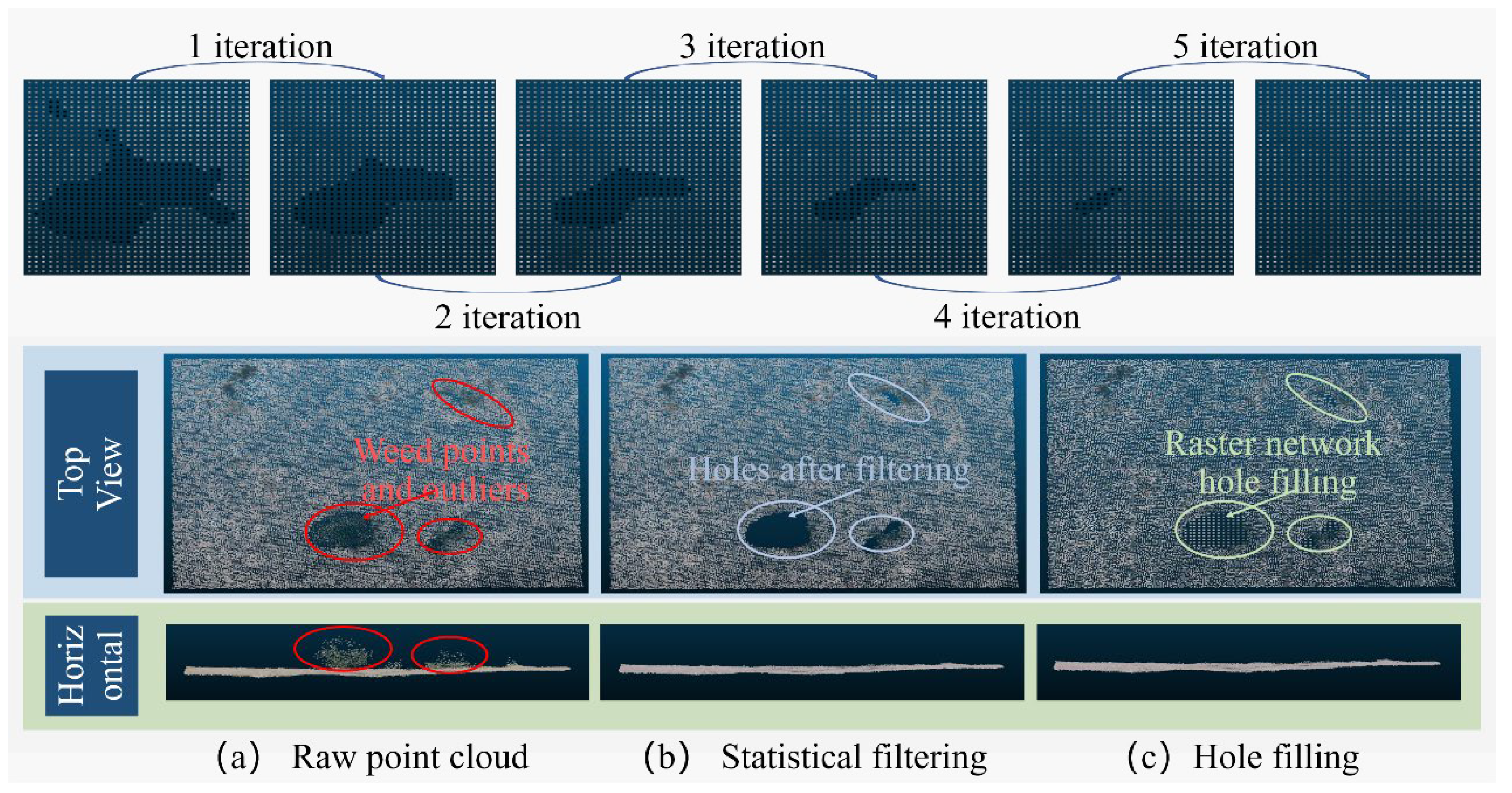
Following the removal of weed-associated point clouds, certain lacunae may manifest within the terrain point cloud. Remedying these voids is imperative to achieving an intact terrain point cloud representation. To this end, the study leverages the region-growing technique to address the task of point cloud cavity completion. Commencing from the periphery of the cavity and progressing inward, the expansion of points is orchestrated on a rasterized grid.
To ensure algorithm efficiency and match the downsampling resolution of the subsequent digital gradient model, the grid side length of the network is selected as 4 cm. The elevation value of the growing point P (the Z coordinate) is used to complete the hole. The formula for calculating is as follows:
in the formula, is the total number of points in the neighborhood point cloud, and l is the side length of the neighborhood window.
The hole-filling point cloud growing algorithm runs inward from the hole boundary in a single iteration. Through multiple iterations, the point cloud holes can be filled, as depicted in Figure 6.

Figure 6.
Region growing iterative hole filling in grid networks.
2.3. Segmentation of Primary Obstacles Based on a Digital Gradient Model
- Digital Gradient Model Construction and Obstacle Semantic Labeling Based on the Sobel-G Operator
In order to depict the morphological attributes of the terrestrial surface relief, the augmented point cloud map is transformed into a digital elevation model. To harness the elevation data effectively, a computation of gradients is executed for every individual point, thereby yielding a digital gradient model. Within this study, a tailored adaptation of the Sobel operator, denoted as the Sobel-G operator, has been devised to approximate the absolute gradient magnitude.
The coefficient matrix of the Sobel-G operator is expressed as a discrete gradient calculation formula:
in the formula, and are the point coordinates of the elevation information, and is the side length of the operator grid.
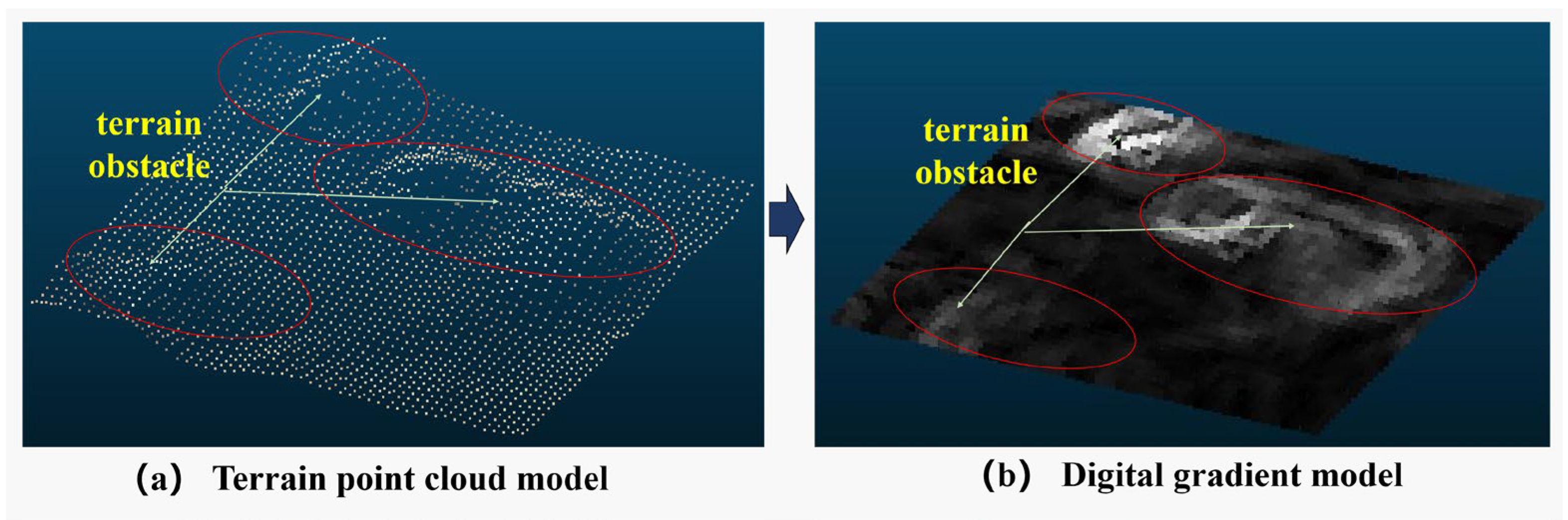
The digital gradient model is constructed by applying the Sobel-G operator to the digital elevation model. The gradient values in the digital gradient model are then converted to grayscale for visualization and further processing. Figure 7 shows the terrain obstacles’ contours clearly observed in the digital gradient model.
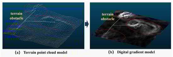
Figure 7.
A digital gradient model constructed by the Sobel-G operator.
Subsequent to the derivation of the digital gradient model through the utilization of the Sobel-G operator, a subsequent phase entails the partitioning of terrain impediments along their boundaries. Within the scope of this research, the OTSU segmentation algorithm is deployed to effectuate the partitioning of concave-convex barriers based on the gradient model. As illustrated in Figure 8, the segmentation outcomes reveal the accurate identification of three obstacles within the non-structured terrain through the employment of gradient model-based segmentation. In contrast, only two larger obstacles are discernible from the elevation model. Furthermore, the boundaries demarcating the segmented obstacles are characterized by enhanced precision when employing the gradient model-based segmentation approach.
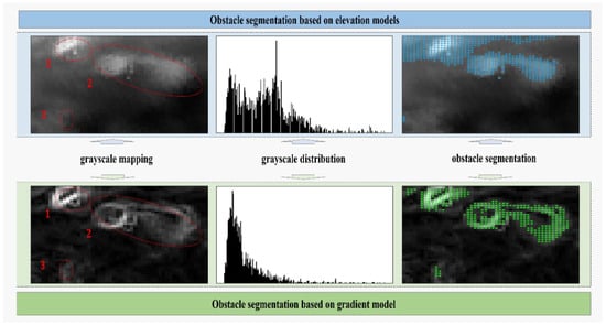
Figure 8.
Comparison of semantic segmentation effects based on the elevation model and the gradient model.
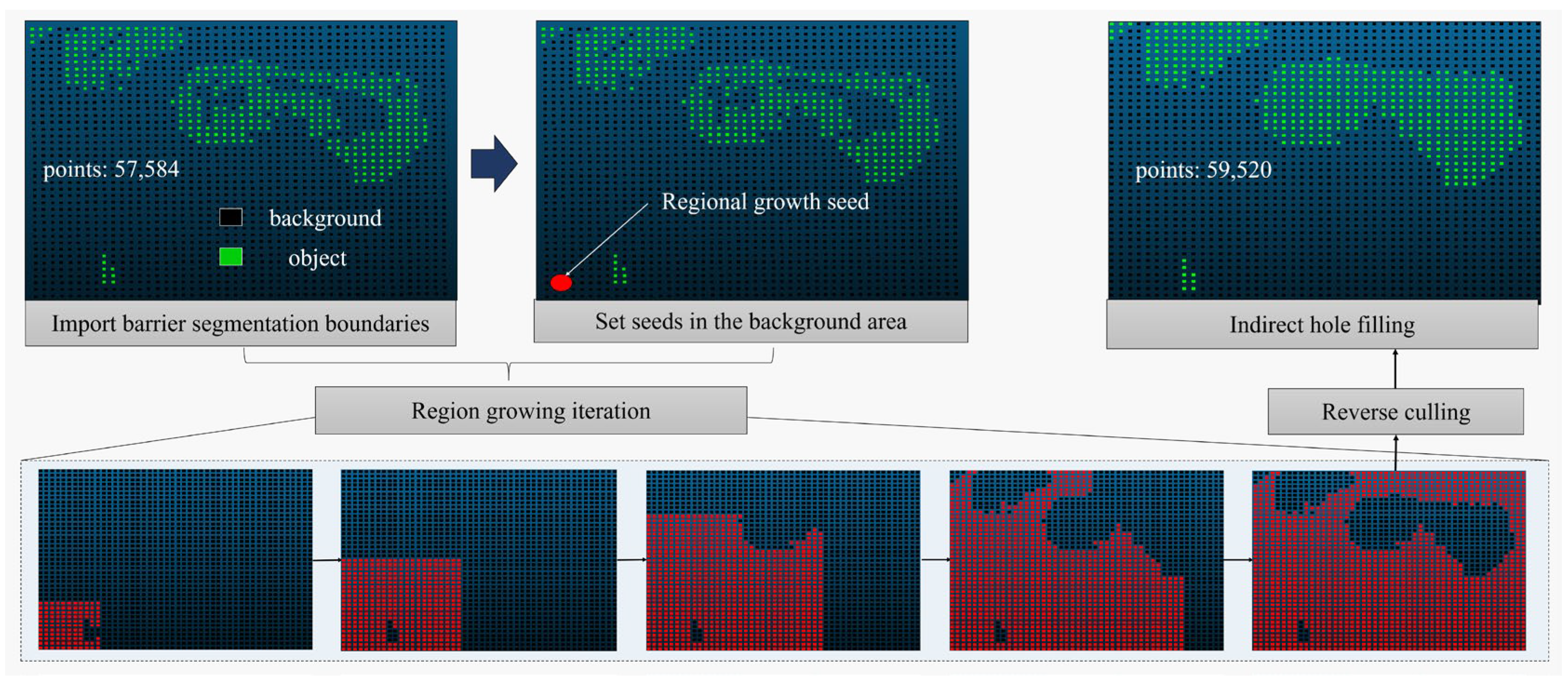
- Indirect hole filling based on background region culling
The obstacle boundaries obtained from the gradient segmentation often contain hollow regions, as shown in Figure 9. Distinguishing between the background area and the hollow area can be challenging based solely on algorithm logic. Direct completion of these regions may lead to incorrect filling. To address this issue, this paper proposes an indirect hole filling Algorithm 1 based on background area culling. The algorithm indirectly obtains the complete obstacle target area by identifying the complete background area. The algorithmic steps are as follows:
| Algorithm 1 Indirect hole filling for obstacles in boundary models |
Input: Obstacle_Boundary_Model(OB) Output: Obstacle_Model(O) Start:
End |

Figure 9.
Indirect hole filling based on background region culling.
The algorithm starts by obtaining the obstacle boundary based on the segmentation of the digital gradient model. By setting area growth seeds, growing them to cover the background area, and subsequently removing the background area, the complete semantic information of the target obstacle is indirectly obtained. In cases where the background area A is large or discontinuous, multiple regional growth seeds can be set to ensure the timeliness and integrity of the background area extraction.
2.4. Point Cloud Segmentation Based on Bi-LSTM Neural Network
- The deep learning network framework for point cloud tuning
After completing the aforementioned steps, the semantic information of the geometric features of the target obstacle’s point cloud in the unstructured environment is fully extracted. To efficiently extract obstacles of the same type from the point cloud, we manually labeled the extracted obstacle information and employed a bidirectional long short-term memory (Bi-LSTM) deep learning method based on a bidirectional recurrent neural network to analyze the target features. The structure of the network is illustrated in Figure 10. The key components include a sequence input layer, a bidirectional long- and short-term memory layer with 300 hidden units, a fully connected layer, a classification layer, and a softmax layer.
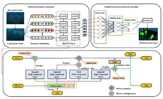
Figure 10.
Flow chart of point cloud segmentation based on the Bi-LSTM neural network.
During the network training process, the forget gate is responsible for discarding redundant information, the input gate updates the relevant point cloud feature information, and the output gate performs long- and short-term memory computations. The cyclic arrangement of these three gates enables the LSTM to learn how to balance the proportion of long- and short-term memory. The choice of a bidirectional long short-term memory neural network is driven by our intention to express the relationship between each point and its neighboring points in a sequential logic format, which better represents the geometry around the point cloud and the interactions between feature vectors. For each point, we identify its neighbors and input them into the deep learning algorithm as a sequence. To ensure training and semantic segmentation accuracy, we incorporate the scattered coordinates of each point in addition to considering the geometric features of the points within the point cloud sequence.
In comparison to traditional recurrent neural network models and LSTM models, which only propagate information forward, the Bi-LSTM model allows for the inclusion of context information more comprehensively at each time step. By leveraging a bidirectional recurrent neural network composed of LSTM neuron models, the Bi-LSTM model can capture contextual information with greater precision.
- Implementation process for applicable point clouds
As mentioned earlier, the implementation of the network is governed by three key gates: forget, input, and output. These gates are responsible for reading, selecting, and forgetting input information. Each gate functions as a fully connected layer, where the input is a vector and the output is a vector of real numbers between 0 and 1. The gate can be expressed as follows:
the (sigmoid) function maps the output values to the range (0–1), making the gate act as a switch that can control the flow of feature information. A gate output of 0 means that the input feature information cannot pass, while an output of 1 allows the feature information to pass through.
The network utilizes two gates to control the content of the unit’s cell state: the forget gate and the input gate. The forget gate determines how much of the previous moment’s unit states are retained in the current moment, while the input gate determines how much of the network’s input is stored in the cell state at the current moment. Finally, the output gate controls the output of the cell state to produce the current output value of the Bi-LSTM.
The specific representation is as follows:
Forget gate:
in the above formula is the weight matrix of the forget gate, and means to connect two vectors into a vector that receives longer information. is the bias term of the forget gate. is the sigmoid function. If the dimension of the input is , the dimension of the hidden layer is , and the dimension of the unit state is , the dimension of the weight matrix of the forget gate is . In order to allow more feature information from the point cloud to be acquired by the network, the weight matrix of this network concatenates the two matrices together. One is , which corresponds to the input item , and its dimension is . The other is , which corresponds to the input item , and its dimension is . Therefore, the of this paper can be written as:
input gate:
in the above formula is the weight matrix of the input gate, and is the bias term of the input gate. is the cell state of the current input, which is calculated based on the previous output and the current input.
After obtaining the current input cell state , the cell state at the current moment can be calculated. It is generated by multiplying the last unit state elementwise by the forget gate, multiplying the current input unit state elementwise by the input gate, and adding the two products. As shown in the following formula:
the symbol indicates element-wise multiplication.
In this way, we combine the LSTM’s current memory and long-term memory to form a new cell state. For the control of the forget gate, it can save the feature information of the long sequence point cloud for a long time. At the same time, the control of the input gate can prevent redundant interference information from entering the memory.
Output gate:
where is the weight matrix of the output gate and is the bias term of the output gate.
The predicted output of the final point cloud feature, determined by the output gate and the cell state:
2.5. Semantic Segmentation of Hazardous Obstacles Based on Vehicle-Terrain Model
To further identify hazardous obstacles within the primary obstacles, the static rollover motion of articulated engineering vehicles is taken into consideration. This part builds upon our previous work and has been further optimized. The articulated engineering vehicle in this paper is a scaled prototype of a real articulated wheeled loader, as depicted in Figure 11a. It possesses a variable structure, a variable mass center, and variable load characteristics. The vehicle’s kinematic model is established with the steering hinge point as the coordinate origin, as shown in Figure 11b.
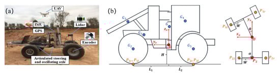
Figure 11.
Coordinate system for an articulated engineering vehicle. (a) The scaled prototype of a real articulated wheeled loader. (b) Schematic diagram of kinematic model coordinates.
The vehicle’s total mass is primarily distributed among different body parts: front body mass G1, front wheel mass G2, front swing arm mass G3, rear body mass G4, and rear wheel mass G5. The center of gravity of the vehicle (x0, y0, z0) is determined by the following equation:
here represents the mass of each vehicle body part, and denotes the coordinates of each vehicle body part.
In order to determine the grounding points of the tires, their coordinates must be determined. These include the left front wheel P1l(x1l, y1l, z1l), right front wheel P1r(x1r, y1r, z1r), left rear wheel P2l(x2l, y2l, z2l), and right rear wheel P2r(x2r, y2r, z2r), expressed as:
in the above equations, represents half the track width. and represent the distances from the front and rear axles to the center of gravity, respectively; H denotes the height of the steering hinge point; represents the articulated steering angle; and represents the rear axle swing angle.
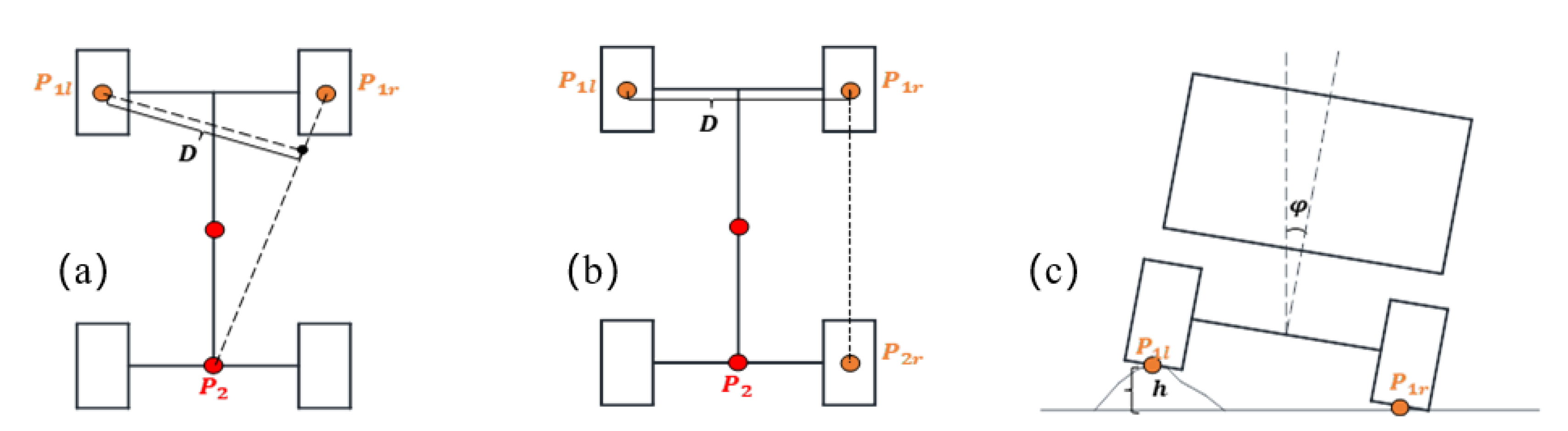
To account for the influence of obstacle elevation on vehicle trafficability, invalid obstacles that do not directly affect the driving stability of engineering vehicles are filtered out by calculating the roll angle threshold as the vehicle crosses obstacles. For this purpose, a critical height threshold is defined to assess the height of hazardous obstacles obtained from the digital elevation model. The static rollover process of articulated engineering vehicles is illustrated in Figure 12.
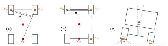
Figure 12.
Static rollover process of an articulated engineering vehicle. (a) Tilting of the vehicle around P1lP2. (b) Tilting of the vehicle around P1lP2r. (c) Vehicle state during obstacle surpassing.
As the vehicle’s wheels maneuver over an obstacle, the vehicle body will roll around the P1rP2 axis when the roll angle is less than the restraint angle of the rear oscillating axle. The roll angle generated at low speed is defined as:
here represents the obstacle height, and is the projection distance from P1l to the P1rP2 axis.
Upon surpassing the prescribed rotational threshold of the rear oscillating axle, the vehicle’s orientation experiences a roll maneuver about the P1rP2r axis, where the parameter D equates to twice the vehicle width (D = 2W). The vehicle transits between these dual states throughout the rollover sequence, with the upper limit of the permissible roll angle computable either through vehicle geometric attributes or empirical data obtained from rollover test benches. Consequently, a designated safety factor δ is introduced to deduce the critical obstacle height, as outlined by the following expression:
by computing the limit roll angle of the scaled prototype vehicle, the invalid obstacles at low speed are filtered out using the elevation model, and the hazardous obstacles are further extracted in the terrain mapping. Figure 13 illustrates the semantic information of hazardous obstacles in a site with dense obstacles, effectively expanding the vehicle’s passable area.
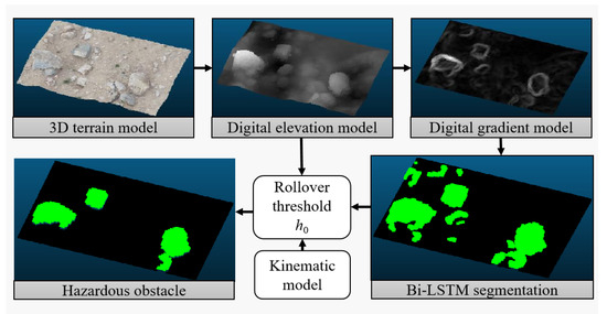
Figure 13.
Semantic segmentation of hazardous obstacles.
3. Experiment and Result Analysis
3.1. Datasets and Evaluation Metrics
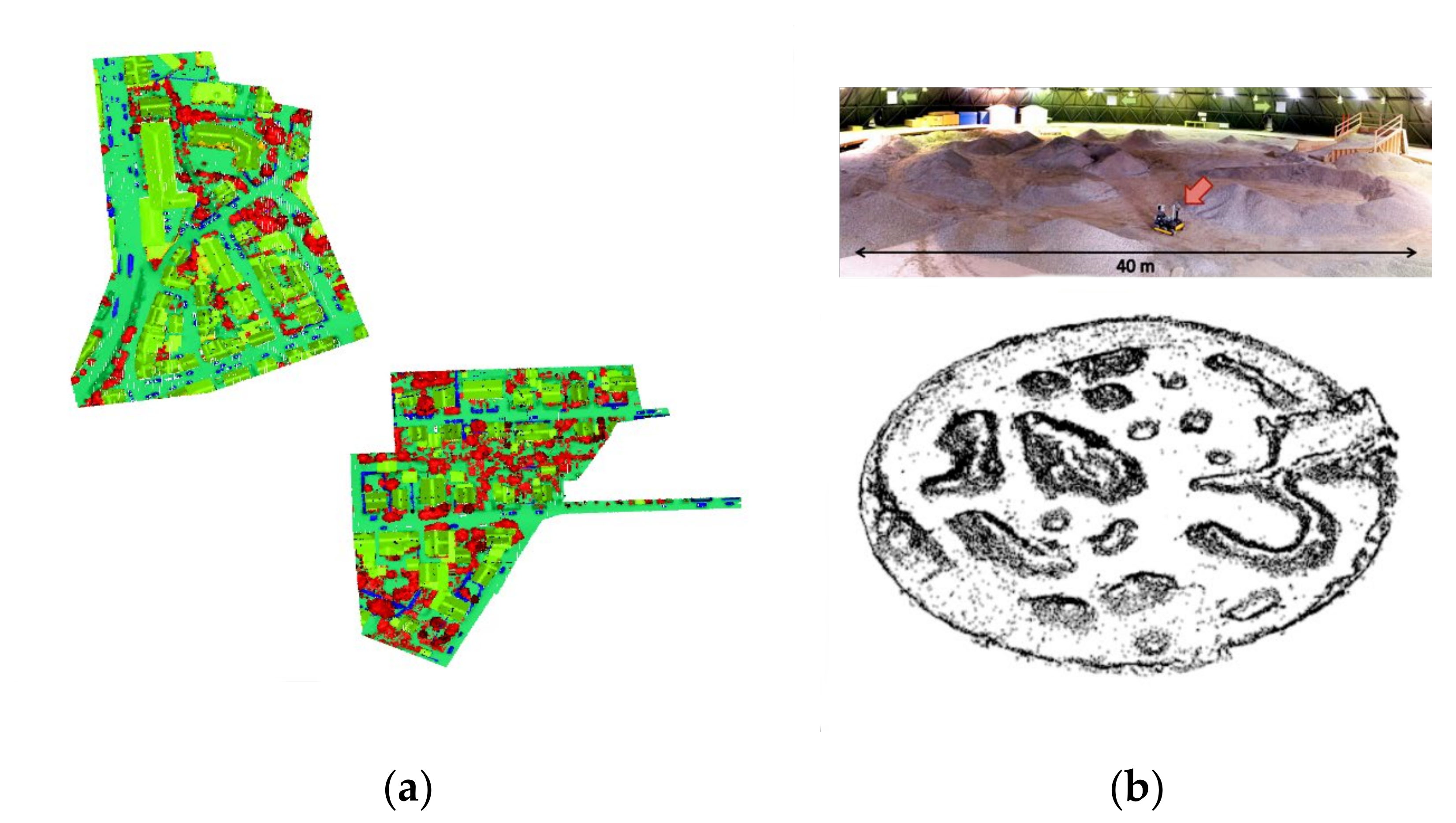
To evaluate the effectiveness of the algorithm framework proposed in this paper, experiments were conducted on self-collected and calibrated datasets as well as two authoritative datasets for further validation, as depicted in Figure 14. The first dataset used for verification is the ISPRS 3D semantic labeling contest dataset, where the extraction effectiveness of the proposed Bi-LSTM neural network is tested. This dataset consists of point cloud data acquired using a Leica ALS50 airborne laser scanner over Vaihingen. The points in the dataset have not been rasterized or post-processed. The dataset provides point labels for nine classes, including powerlines, low vegetation, impervious surfaces, cars, fences/hedges, roofs, facades, shrubs, and trees.

Figure 14.
Dataset used for testing. (a) The ISPRS 3D semantic labeling contest dataset. (b) The Canadian planetary emulation terrain 3D mapping dataset.
The second dataset used for verification is the Canadian planetary emulation terrain 3D mapping dataset, which aims to assess the obstacle detection effect of the segmentation network combined with vehicle kinematic modeling technology. This dataset comprises 95 laser scans obtained at the University of Toronto Institute for Aerospace Studies (UTIAS) indoor rover test facility in Toronto, Ontario, Canada. The test facility includes a large dome structure that covers a circular workspace area with a diameter of 40 m. Within this workspace, gravel was distributed to emulate scaled planetary hills and ridges, providing a characteristic natural and unstructured terrain.
For the tests conducted on these datasets, three evaluation metrics were employed to quantify the detection effectiveness of the proposed method: Recall, Precision, and F1-measure. Recall measures the true positive rate, representing the percentage of correctly identified positives in the ground truth. Precision measures the positive predictive value, representing the percentage of correctly identified positives out of the total identified positives. F1-measure is a combined performance metric that considers both Recall and Precision. The specific expressions of these metrics are as follows:
here TP represents the number of true positives, FN represents the number of false negatives, and FP represents the number of false positives in the point cloud data. These metrics provide a comprehensive assessment of the detection performance of the proposed method.
3.2. Obstacle Detection Results of the Image Point Cloud
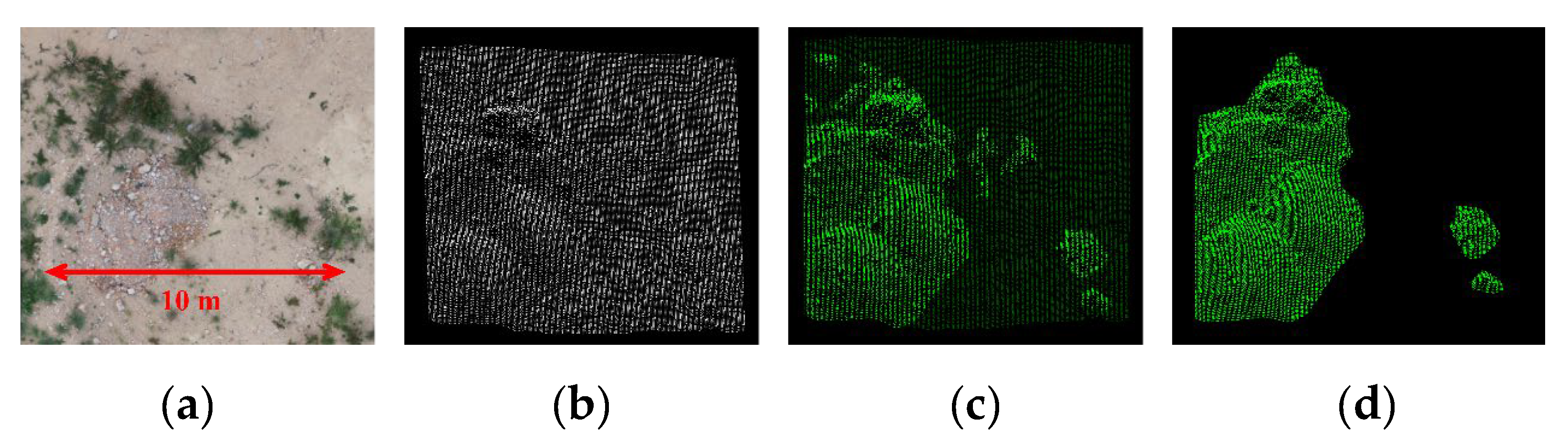
The results of our proposed approach for risky obstacle detection on the validation set of the drone-generated image point cloud model are presented in Figure 15 and Figure 16. These figures depict the predicted obstacle detection outcomes. The performance of our method is comprehensively evaluated using three metrics: Precision, Recall, and F1-score. The performance values are summarized in Table 2.
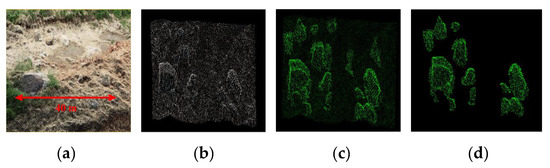
Figure 15.
UAV aerial image point cloud dataset. (a) Medium scale unstructured scene. (b) Point cloud view. (c) Ground truth view. (d) Hazardous obstacle prediction result.
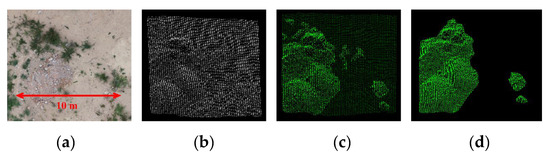
Figure 16.
UAV aerial image point cloud dataset. (a) Small scale, unstructured scene. (b) Point cloud view. (c) Ground truth view. (d) Hazardous obstacle prediction result.
Table 2.
Hazardous obstacle prediction result for a medium scale unstructured scene.
Among these indicators, for the detection of dangerous obstacles, our method achieved a Precision of 93.99%, Recall of 89.15%, and an F1-score of 91.51%. These results demonstrate that our method exhibits highly accurate and reliable performance on the annotated dataset.
The visual representations in Figure 15 and Figure 16, combined with the quantitative evaluation in Table 2, highlight the effectiveness and robustness of our proposed approach for obstacle detection in the image point cloud. The achieved performance metrics indicate that our method is capable of accurately identifying and segmenting risky obstacles, providing a solid foundation for safe driving decision-making in unstructured terrain environments.
3.3. Classification Results of the ISPRS 3D Semantic Labeling Contest Dataset
To assess the holistic efficacy of the proposed Bi-LSTM neural network, a series of assessments were carried out on the ISPRS 3D semantic labeling contest dataset. The outcomes of the classification process are meticulously documented, with the corresponding confusion matrix presented in Table 3 and Figure 17. Furthermore, a visual depiction of the classification outcomes is furnished in Figure 18.
Table 3.
Confusion matrix of our method based on the ISPRS benchmark testing data. Precision, Recall, and F1 scores are shown for each category.
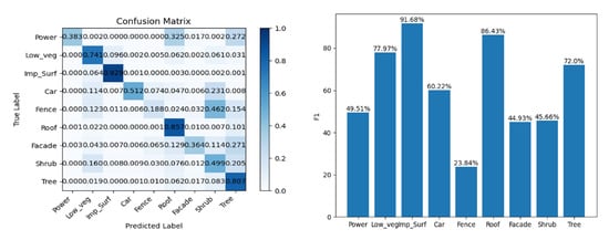
Figure 17.
Confusion matrix and F1 score of our method on the ISPRS benchmark testing data.
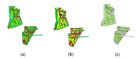
Figure 18.
Prediction results of the ISPRS 3D semantic labeling contest dataset by the Bi-LSTM neural network. (a) Ground truth. (b) Prediction results. (c) Predicted results for roofs and roads only.
Remarkably, our method accomplished accurate predictions for 67% of the test points, encompassing clearly defined categories such as Imp_Surf and Roof. This notable achievement can be attributed to the synergistic amalgamation of distinctive features and the temporal sequence training embedded within our methodology.
Table 4 presents a quantitative comparative analysis between our proposed approach and several contemporary, comprehensive classification methodologies utilizing the ISPRS dataset. The examined methodologies encompass the machine learning-based DT+GMM method alongside deep learning-based strategies such as DGCNN, alsNet, HA-GCN, and RandLA-Net.
Table 4.
Quantitative comparisons on the ISPRS 3D semantic labeling contest dataset. The numbers in the first nine columns present the F1 scores for different categories. The average F1 score (Avg. F1) is listed in the last column.
In contrast to the machine learning paradigm represented by DT+GMM, our deep learning approach yields a notably elevated average F1-score of 0.614, attesting to its superior efficacy in the domain of point cloud processing and classification. Furthermore, in contrast to the foundational deep learning framework of PointNet, our proposed approach demonstrates commendable competitive attributes, manifesting superior classification performance.
Compared to DGCNN, which prioritizes local feature acquisition between data points, and alsNet, characterized by an encoding-decoding architecture, our deeper network structure yields discernible computational efficiency enhancements. By leveraging Bi-LSTM networks to train classifier features as a recognition sequence, our approach attains superior average F1-scores relative to DGCNN and alsNet, surpassing them by margins of 0.017 and 0.01, respectively.
While a noticeable disparity persists between our approach and the advanced methodologies of HA-GCN and RandLA-Net, our technique remains a viable contender, particularly within categories characterized by well-defined features like Imp_Surf. This observed gap can be attributed to the adoption of extensive, multi-tiered network architectures in recent algorithms, benefiting from potent GPUs to enhance point cloud processing. Conversely, our proposed methodology presents a compact model size and abbreviated training time, rendering it efficacious and cost-efficient for practical implementation. The training process consumes approximately 10 min, and the model’s dimensions are confined to a mere 5 MB, negating the necessity for GPU-based training.
In summation, the classification outcomes gleaned from the ISPRS dataset affirm both the effectiveness and efficiency of our proposed Bi-LSTM neural network approach in semantic segmentation endeavors. This substantiates its prospective utility in facilitating comprehensive point cloud analysis and classification, with implications extending across diverse application domains.
3.4. Classification Results of the Canadian Planetary Emulation Terrain 3D Mapping Dataset
Figure 19 showcases the obstacle detection results obtained from the Canadian Planetary Emulation Terrain 3D Mapping dataset. A comparison is made between Chen’s latest method and our proposed method for obstacle detection. Chen’s method is depicted in Figure 19b. As can be observed, his obstacle detection method, which relies on a clustering algorithm, fails to accurately detect obstacles due to the black point clouds in the dataset not being completely separated.
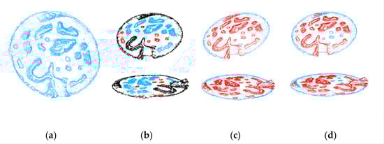
Figure 19.
Obstacle detection results on the Canadian Planetary Emulation Terrain 3D Mapping dataset. (a) Ground truth of the dataset. (b) Chen’s method [34]. (c) Prediction results of Bi-LSTM. (d) Hazardous obstacle detection results combined with vehicle dynamics.
On the other hand, Figure 19c presents the prediction results of our neural network-based obstacle detection method. By leveraging deep learning, our approach overcomes the limitations of traditional clustering algorithms that can only detect specific datasets and classified objects. Our method demonstrates the ability to detect more comprehensive obstacles, showcasing the algorithm’s generalizability to different data.
Furthermore, Figure 19d displays the prediction results of hazardous obstacles that impact driving safety, combining the dynamics of the vehicle’s geometry. In contrast to the global obstacle detection method, our approach, which incorporates dynamic hazardous obstacle prediction, provides the optimal path for vehicles to navigate through, ensuring their safety during the driving process.
Overall, the results obtained from the Canadian Planetary Emulation Terrain 3D Mapping dataset demonstrate the effectiveness of our proposed method in detecting obstacles and predicting hazardous obstacles. The combination of deep learning-based obstacle detection and vehicle geometry dynamics contributes to improved obstacle detection accuracy and enhanced safety in driving scenarios.
3.5. Engineering Applications of the Hazardous Obstacle Detection Framework
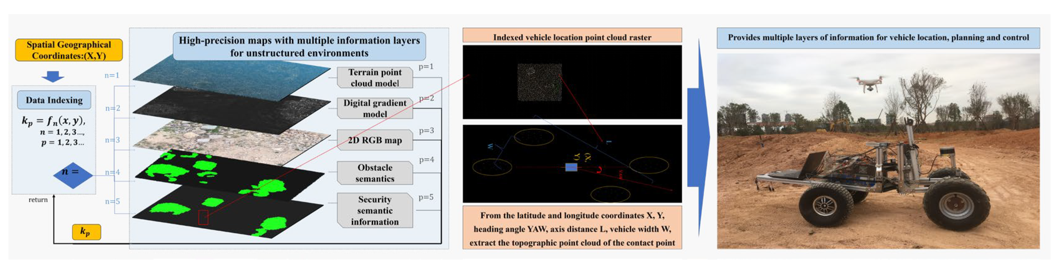
Figure 20 demonstrates the practical application of our hazardous obstacle detection framework in the rapid construction of high-precision maps for unmanned engineering vehicles in unstructured environments. This framework effectively tackles the challenges faced in unstructured environments by utilizing UAV oblique photography techniques to construct terrain point clouds. By employing UAVs instead of vehicle-mounted platforms, we overcome the difficulties associated with driving on unstructured terrain and the high vibration that can impact modeling accuracy. This approach also meets the demand for rapid and periodic modeling of dynamically changing unstructured surfaces.

Figure 20.
Engineering applications of a safety-assured semantic map.
The framework incorporates various steps to enhance the accuracy and usefulness of the constructed maps. Initially, statistical filtering is applied in both geometric and color spaces to remove outliers and ground-weed point clouds. This pre-processing step optimizes the appearance of the terrain point cloud and establishes a formatted data model that facilitates indexing and further analysis.
Semantic segmentation of obstacles is achieved through deep learning-based techniques. This step provides rich semantic information regarding the regional driving safety level. By constructing a vehicle-terrain contact coupling model, static stability indicators are calculated, enabling the segmentation of driving safety levels. This additional semantic information enhances the design of autonomous driving decision-making and control systems for engineering vehicles.
In engineering scenarios, our framework enables the rapid and accurate construction of high-precision maps in unstructured environments. It addresses the specific challenges associated with such environments, improves the quality of modeling, and provides valuable semantic information for the design of autonomous driving decision-making and control systems for engineering vehicles. By incorporating advanced technologies, our framework enhances the safety and efficiency of unmanned engineering vehicle operations in complex terrain.
4. Conclusions
In this paper, we have presented a comprehensive framework for hazardous obstacle detection in unstructured environments using drone-based modeling. It is a combined method of innovation where the synergistic integration of various techniques contributes to a novel and effective approach. By leveraging the advantages of drones, such as low cost, speed, and periodicity, we have successfully addressed the challenges associated with modeling large-scale unstructured scenarios. Through point cloud filtering and the application of deep learning algorithms for obstacle identification, we have significantly improved the availability of obstacle semantic information. Furthermore, we have incorporated a vehicle-terrain dynamics model specific to articulated engineering vehicles to extract hazardous obstacles that pose a threat to vehicle safety. By integrating this information into high-precision maps, our framework provides valuable semantic and vehicle safety information for autonomous engineering vehicles. This enhances their ability to navigate and make informed decisions in complex environments. Moving forward, our future research will focus on developing path tracking algorithms based on high-precision maps with semantic information about hazardous obstacles. By further advancing the capabilities of our framework, we aim to improve the path planning and decision-making processes for engineering vehicles operating in unstructured environments.
Author Contributions
Conceptualization, S.S., Q.Z., and T.H.; methodology, S.S.; software, S.S.; validation, S.S. and C.L.; formal analysis, G.S.; investigation, Q.Z.; resources, S.S. and T.H.; data curation, G.S.; writing—original draft preparation, S.S., Y.G.; writing—review and editing, S.S.; visualization, S.S. and C.L.; supervision, S.S.; project administration, Q.Z.; funding acquisition, Q.Z. All authors have read and agreed to the published version of the manuscript.
Funding
This research was funded by the National Natural Science Foundation of China (grant number 52075461), the National Key Research and Development Program (grant number 2022YFB3206605), the Fujian Province Regional Development Project (grant number 2022H4018), and the Fujian Province University Industry-Academic Cooperation Project (grant number 2021H6019).
Data Availability Statement
Not applicable.
Acknowledgments
The authors would like to thank the Editor-in-Chief, Editor, and anonymous reviewers for their valuable reviews.
Conflicts of Interest
The authors declare no conflict of interest.
References
- Zhang, L.; Zhao, J.; Long, P.; Wang, L.; Qian, L.; Lu, F.; Song, X.; Manocha, D. An autonomous excavator system for material loading tasks. Sci. Robot. 2021, 6, 55. [Google Scholar] [CrossRef] [PubMed]
- Ha, Q.P.; Yen, L.; Balaguer, C. Robotic autonomous systems for earthmoving in military applications. Autom. Constr. 2019, 107, 102934. [Google Scholar] [CrossRef]
- Sharma, K.; Zhao, C.; Swarup, C.; Pandey, S.K.; Kumar, A.; Doriya, R.; Singh, K.U.; Singh, T. Early detection of obstacle to optimize the robot path planning. Drones 2022, 6, 10. [Google Scholar] [CrossRef]
- Bai, Y.; Fan, L.; Pan, Z.; Chen, L. Monocular outdoor semantic mapping with a multi-task network. In Proceedings of the IEEE/RSJ International Conference on Intelligent Robots and Systems (IROS), Macau, China, 4–8 November 2019; pp. 1992–1997. [Google Scholar]
- Jiang, K.; Yang, D.; Liu, C.; Zhang, T.; Xiao, Z. A flexible multi-layer map model designed for lane-level route planning in autonomous vehicles. Engineering 2019, 5, 305–318. [Google Scholar] [CrossRef]
- Ebadi, K.; Chang, Y.; Palieri, M.; Stephens, A.; Hatteland, A.; Heiden, E.; Thakur, A.; Funabiki, N.; Morrell, B.; Wood, S.; et al. LAMP: Large-scale autonomous mapping and positioning for exploration of perceptually-degraded subterranean environments. In Proceedings of the IEEE International Conference on Robotics and Automation (ICRA), Paris, France, 31 May–31 August 2020; pp. 80–86. [Google Scholar]
- Pan, Y.; Xu, X.; Ding, X.; Huang, S.; Wang, S.; Xiong, R. GEM: Online globally consistent dense elevation mapping for unstructured terrain. IEEE Trans. Instrum. Meas. 2021, 70, 1–13. [Google Scholar] [CrossRef]
- Matthies, L.; Maimone, M.; Johnson, A.; Cheng, Y.; Willson, R.; Villalpando, C.; Goldberg, S.; Huertas, A.; Stein, A.; Angelova, A. Computer vision on Mars. Int. J. Comput. Vis. 2007, 75, 67–92. [Google Scholar] [CrossRef]
- Cheng, Y.; Maimone, M.W.; Matthies, L. Visual odometry on the Mars exploration rovers-a tool to ensure accurate driving and science imaging. IEEE Robot. Autom. Mag. 2006, 13, 54–62. [Google Scholar] [CrossRef]
- Ma, J.; Bajracharya, M.; Susca, S.; Matthies, L.; Malchano, M. Real-time pose estimation of a dynamic quadruped in GPS-denied environments for 24-hour operation. Int. J. Robot. Res. 2016, 35, 631–653. [Google Scholar] [CrossRef]
- Bernuy, F.; del Solar, J.R. Semantic mapping of large-scale outdoor scenes for autonomous off-road driving. In Proceedings of the IEEE International Conference on Computer Vision Workshops(ICCVW), Santiago, Chile, 11–18 December 2015; pp. 35–41. [Google Scholar]
- Sock, J.; Kim, J.; Min, J.; Kwak, K. Probabilistic traversability map generation using 3D-LIDAR and camera. In Proceedings of the IEEE International Conference on Robotics and Automation (ICRA), Stockholm, Sweden, 16–21 May 2016; pp. 5631–5637. [Google Scholar]
- Jamali, A.; Anton, F.; Rahman, A.A.; Mioc, D. 3D indoor building environment reconstruction using least square adjustment, polynomial kernel, interval analysis and homotopy continuation. In Proceedings of the 3rd International GeoAdvances Workshop/ISPRS Workshop on Multi-dimensional and Multi-Scale Spatial Data Modeling, Istanbul, Turkey, 16–17 October 2016; pp. 103–113. [Google Scholar]
- Milella, A.; Cicirelli, G.; Distante, A. RFID-assisted mobile robot system for mapping and surveillance of indoor environments. Ind. Robot. 2008, 35, 143–152. [Google Scholar] [CrossRef]
- Xia, X.; Meng, Z.; Han, X.; Li, H.; Tsukiji, T.; Xu, R.; Zheng, Z.; Ma, J. An automated driving systems data acquisition and analytics platform. Transp. Res. Pt. C-Emerg. Technol. 2023, 151, 104120. [Google Scholar] [CrossRef]
- Shan, T.; Englot, B. LeGO-LOAM: Lightweight and ground-optimized lidar odometry and mapping on variable terrain. In Proceedings of the IEEE/RSJ International Conference on Intelligent Robots and Systems (IROS), Madrid, Spain, 1–5 October 2018; pp. 4758–4765. [Google Scholar]
- Le Gentil, C.; Vayugundla, M.; Giubilato, R.; Stürzl, W.; Vidal-Calleja, T.; Triebel, R. Gaussian process gradient maps for loop-closure detection in unstructured planetary environments. In Proceedings of the IEEE/RSJ International Conference on Intelligent Robots and Systems (IROS), Las Vegas, NV, USA, 24 October 2020–24 January 2021; pp. 1895–1902. [Google Scholar]
- Casella, V.; Franzini, M. Modelling steep surfaces by various configurations of nadir and oblique photogrammetry. In Proceedings of the 23rd ISPRS Congress, Prague, Czech Republic, 12–19 July 2016; Volume 3, pp. 175–182. [Google Scholar]
- Ren, J.; Chen, X.; Zheng, Z. Future prospects of UAV tilt photogrammetry technology. In IOP Conference Series: Materials Science and Engineering; IOP: Bristol, UK, 2019; Volume 612, p. 032023. [Google Scholar]
- Liu, Y.; Zheng, X.; Ai, G.; Zhang, Y.; Zuo, Y. Generating a high-precision true digital orthophoto map based on UAV images. ISPRS Int. J. Geo-Inf. 2018, 7, 333. [Google Scholar] [CrossRef]
- Liu, J.; Xu, W.; Guo, B.; Zhou, G.; Zhu, H. Accurate mapping method for UAV photogrammetry without ground control points in the map projection frame. IEEE Trans. Geosci. Remote Sens. 2021, 5, 9673–9681. [Google Scholar] [CrossRef]
- Li, X.; Wu, Y.; Zhou, W.; Yao, Z. Study on roll instability mechanism and stability index of articulated steering vehicles. Math. Probl. Eng. 2016, 2016, 7816503. [Google Scholar] [CrossRef]
- Zhu, Q.; Chen, W.; Hu, H.; Wu, X.; Xiao, C.; Song, X. Multi-sensor based attitude prediction for agricultural vehicles. Comput. Electron. Agric. 2019, 156, 24–32. [Google Scholar] [CrossRef]
- Zhang, X.; Liu, Q.; Liu, J.; Zhu, Q.; Hu, H. Using gyro stabilizer for active anti-rollover control of articulated wheeled loader vehicles. Proc. Inst. Mech. Eng. Part I-J. Syst Control Eng. 2021, 235, 237–248. [Google Scholar] [CrossRef]
- Ghotbi, B.; González, F.; Kövecses, J.; Angeles, J. Vehicle-terrain interaction models for analysis and performance evaluation of wheeled rovers. In Proceedings of the IEEE/RSJ International Conference on Intelligent Robots and Systems (IROS), Algarve, Portugal, 7–12 October 2012; pp. 3138–3143. [Google Scholar]
- Choi, Y.; Kim, H. Convex hull obstacle-aware pedestrian tracking and target detection in theme park applications. Drones 2023, 7, 279. [Google Scholar] [CrossRef]
- Meng, Z.; Xia, X.; Xu, R.; Liu, W.; Ma, J. Hydro-3d: Hybrid object detection and tracking for cooperative perception using 3d lidar. IEEE T Intell. Veh. 2023, 1–13. [Google Scholar] [CrossRef]
- Qi, C.; Su, H.; Mo, K.; Guibas, L. PointNet: Deep Learning on Point Sets for 3D Classification and Segmentation. In Proceedings of the IEEE/CVF Conference on Computer Vision and Pattern Recognition (CVPR), Honolulu, HI, USA, 21–26 July 2017; pp. 652–660. [Google Scholar]
- Liu, X.Q.; Chen, Y.M.; Li, S.Y.; Cheng, L.; Li, M.C. Hierarchical Classification of Urban ALS Data by Using Geometry and Intensity Information. Sensors 2019, 19, 4583. [Google Scholar] [CrossRef]
- Wang, Y.; Sun, Y.B.; Liu, Z.W.; Sarma, S.E.; Bronstein, M.M.; Solomon, J.M. Dynamic graph cnn for learning on point clouds. ACM Trans. Graph. 2019, 38, 1–12. [Google Scholar] [CrossRef]
- Winiwarter, L.; Mandlburger, G.; Schmohl, S.; Pfeifer, N. Classification of ALS Point Clouds Using End-to-End Deep Learning. PFG-J. Photogramm. Remote Sens. Geoinf. Sci. 2019, 87, 75–90. [Google Scholar] [CrossRef]
- Wen, P.; Cheng, Y.L.; Wang, P.; Zhao, M.J.; Zhang, B.X. HA-GCN: An als point cloud classification method based on height-aware graph convolution network. In Proceedings of the 13th International Conference on Graphics and Image Processing (ICGIP), Yunnan Univ, Kunming, China, 18–20 August 2022; p. 12083. [Google Scholar]
- Hu, Q.; Ang, B.; Xie, L.; Rosa, S.; Markham, A. RandLA-Net: Efficient semantic segmentation of large-scale point clouds. In Proceedings of the IEEE/CVF Conference on Computer Vision and Pattern Recognition (CVPR), Seattle, WA, USA, 13–19 June 2020; pp. 11108–11117. [Google Scholar]
- Chen, W.; Liu, Q.; Hu, H.; Liu, J.; Wang, S.; Zhu, Q. Novel laser-based obstacle detection for autonomous robots on unstructured terrain. Sensors 2020, 20, 18. [Google Scholar] [CrossRef]


Disclaimer/Publisher’s Note: The statements, opinions and data contained in all publications are solely those of the individual author(s) and contributor(s) and not of MDPI and/or the editor(s). MDPI and/or the editor(s) disclaim responsibility for any injury to people or property resulting from any ideas, methods, instructions or products referred to in the content. |
© 2023 by the authors. Licensee MDPI, Basel, Switzerland. This article is an open access article distributed under the terms and conditions of the Creative Commons Attribution (CC BY) license (https://creativecommons.org/licenses/by/4.0/).