Coupling Dynamics Study on Multi-Body Separation Process of Underwater Vehicles

Abstract

Based on the Newton-Euler method, a coupling rigid-body dynamics model of a Trans-Medium Vehicle (TMV) separating from an Unmanned Underwater Vehicle (UUV) has been established. The modeling is based on the “holistic method” and “Kane” ideas respectively, so that most of the equations can be derived without considering the internal forces between the two bodies. The separation propulsion force, which is an internal force, only appears in the relative glide dynamics equation of the TMV along the axis of the separation tube that is installed on the UUV. This greatly reduces the workload of modeling and derivation. The UUV works entirely underwater, while the hydrodynamic shape of the TMV changes continuously during the process of the TMV separating from the UUV. Therefore, accurate hydrodynamic calculations for the UUV and TMV are the basis of numerical resolution for the two rigid bodies’ coupling dynamics model in water. A large number of numerical simulations was conducted using CFD methods to investigate the hydrodynamic performance of the UUV and TMV under various conditions. These simulations aim to establish a hydrodynamic database, and accurate hydrodynamic models were developed through fitting methods and online interpolation. In the process of solving the coupling dynamics of two bodies, the hydrodynamic model is used to calculate the hydrodynamic force experienced by the UUV and TMV. This balances the accuracy and efficiency of a numerical simulation. Finally, numerous simulations and comparative analyses were conducted under various operational conditions and separation parameters. The simulation results indicate that the impact of TMV separation on the motion state of the UUV becomes more prominent with smaller UUV to TMV mass ratios or deeper TMV separation depths. This effect can further influence the stability control of the UUV. The coupling rigid body dynamics analysis method established in this paper provides a fast and effective prediction method for use during the scheme design and separation safety evaluation phases of creating UUV-TMV systems.

1. Introduction

With the increasing intelligence and capabilities of unmanned detection equipment, Unmanned Underwater Vehicles (UUV) will be widely used in future ocean development, and thus they have become a field in active development in countries around the world. According to current trends in UUV development, typical operational conditions include marine scientific research, resource exploration, search and rescue operations, and support for manned platforms [1]. When the payload carried by a UUV separates from the UUV underwater, strong interactions and couplings occur between the UUV and the payload. For small UUVs, due to their relatively small mass, the coupling effects of payloads significantly affect their attitudes and other motion states, potentially compromising their operational safety. Conversely, the coupling effects of a small UUV on a payload also impact the trajectory, attitude underwater, and even surface emergence and safety of both the UUV and the payload. Therefore, research into the two-body coupling dynamics issues during the separation of Trans-Medium Vehicles (TMV refers to a new type of aircraft that can cross the water-air interface and can stably navigate in water and fly in the air) and UUVs is of significant value.

In the research of the Weiland et al. [2], the optimal rotation angle of an underwater missile launcher was calculated using experimental data, and the optimal launch water depth was determined by simulating the flow field of the missile during the launching process at different launch depths and relative movement velocities. The influence of the wave force on the water trajectory of the carrier when the submarine launches an unpowered carrier was studied by Pan et al. [3], and the stability and control law of the carrier’s motion were analyzed. In the research of Liu et al. [4,5], the ballistic kinematics model of the underwater vertical launch of a missile and the dynamic model of a six-degree-of-freedom missile were established based on the numerical method and Newton’s second law and the moment of momentum theorem, respectively, and the influence of wave force on the underwater trajectory of the missile at different speeds and the related missile control strategies were studied. The pressure distribution characteristics of the tail’s cavitation during the vertical launch of the missile was discussed by Li et al. [6], and the six-degree-of-freedom dynamics equation of the projectile’s body with a tail cavitation bubble was established to analyze the changes of the projectile’s pitch angle and pitch angular velocity under different conditions. References [3,4,5,6] all focus on studying the influence of wave forces on the launched object during the separation process, and this article also focuses on the influence of hydraulic forces on a TMV’s motion during the separation process. Jiang et al. [7] analyzed the motion characteristics of a submarine-launched cruise missile when it is launched vertically in water, and studied the forces that act on a missile in water under different working conditions. A mathematical model of a submarine-launched missile was established in the research of Li et al. [8] to evaluate the effects of boat speed and adapter stiffness on the attitude of the missile. Shang et al. [9] established a dynamics model and proposed a method of numerically calculating the underwater vertical launch process of a missile. They also analyzed the influence of the transverse current on the motion of the missile. In the process of studying a TMV separating from the separation tube, this study also analyzed the influence of lateral water flow on a TMV. Wang et al. [10] studied the trajectory of a missile launched by a submarine and quantitatively analyzed the six-degree-of-freedom trajectory of the missile under three conditions—static flow, constant velocity water flow, and variable velocity water flow—during the simulation process. Their paper argues that water velocity is an important factor that determines the success of the missile launch. The research of You et al. [11], considering the time-variant fluid-structure interaction effects and the nonlinear contact influence at the connections of the segments during the submarine-launched vehicle’s launch process, simplified it to a free-free boundary Timoshenko beam and analyzed the impact of the connection structure, load, and launch speed on the dynamic response characteristics of the underwater vehicle’s structure. In the study of Zahid et al. [12], a two-dimensional model of the underwater launch of the missile was established based on a CFD software. The trajectory of the missile was tracked based on moving grid technology, the numerical simulation of the missile under different masses, different shapes, and different depths was carried out, and the launch pressure under different conditions was determined. The effects of launch conditions and wave interference on the stability of the submersible at the water-air interface were studied by Zhang et al. [13], and a coupling model of the submersible’s out-of-water motion was established using the RNG k-turbulence model and the VOF method. Numerical simulations of the ejection process of the submersible under different initial inclination angles and velocities were carried out, and the effects of the initial inclination angle and initial velocity on the ejection motion of the submersible were obtained. Refs. [12,13] describe a CFD modeling method that has the advantage of obtaining detailed flow field characteristics during the separation process, but the disadvantages of being time-consuming to calculate and difficult to use for the fast calculations of multiple working conditions required in the conceptual design and scheme design stages. In this paper, a hydrodynamic database of a UUV and a TMV is established by CFD simulation, and the hydrodynamic of the UUV and TMV is quickly called and calculated under the multiple working conditions of the simulation. The effects of gas and water flow on the projectile during launch were studied by Cheng et al. [14], and the variation of the free surface of the exhaust bubble over time was analyzed.

The above literature investigated the mechanical and motion characteristics of a separation object during underwater separation from different perspectives, as well as the main influencing factors. The summarized main factors and modeling methods have a certain reference value for this article, but did not take into account the influence of the separation process on the submersible itself.

In terms of control (UUV): Hu et al. [15] established a mathematical model that simulates a submarine underwater launching missiles, simulated and analyzed the missile launch process, and studied the possible control modes adopted by submarines. Tan et al. [16] studied the mechanical environment of the submarine when an UAV (Unmanned Aerial vehicle) is launched horizontally, established a dynamic model of the in-water trajectory, and discussed the emergency avoidance control strategy of the submarine in the event of an aircraft ignition failure. In the research of Bian et al. [17], a ballistic model of the underwater launch and descent of a vehicle with damping plates was established, the ballistics of different launch depths and exit speeds were simulated, and the influence of different factors on the safety of the launch carrier was analyzed. In the study of Lv et al. [18], a simulation model of the vertical launch of a missile was established based on the equation of motion of the submarine. The influence of uncertainties on the missile launch and the control process of the submarine’s state recovery was analyzed according to the numerical simulation results. In order to improve the reliability of the launch of submarine-launched missiles [19], the effects of the submarine’s speed, the sea current to ground speed, and sea state and current direction on the launch depth and exit velocity of the missile were studied by Liu et al. Based on a combination of theoretical analysis and numerical simulation, Li et al. [20] studied the underwater launch, underwater navigation process, and submarine safety of the moving body from multiple perspectives, analyzed the influence of a missile’s launch parameters, model size, and ocean current on the safety of the submarine after launching the missile, and proposed a corresponding control strategy. Refs. [15,16,17,18,19,20] mainly focus on the impact projectile separation has on submarines and provide safety control measures for submarines after launching projectiles. At the same time, the above literature also studied some operating conditions and submarine maneuvering strategies for separating projectiles from submarines, providing a reference for setting TMV separation operating conditions in this paper.

In conclusion, according to the publicly available literature, few scholars have detailed the coupling dynamics equations of UUV-TMVs. This paper employs the Newton-Euler method to establish a coupling rigid-body dynamics model for UUVs and TMVs. The mechanical characteristics of the separation process of the two rigid bodies are analyzed using different separation parameters and mass ratios, which have great reference value for guiding the design of UUV schemes.

The structure of this paper is as follows: Section 1 presents the research’s background and significance. Section 2 derives the coupling dynamics differential equations of UUV-TMVs in detail. Section 3 elucidates the hydraulic force calculation methods and provides the results of some simulation calculations. Section 4 presents numerical simulation results of the coupling dynamics during the separation process. Finally, conclusions are drawn and summarized in Section 5.

2. Coupling Dynamics Modeling of UUV and TMV

2.1. Definition of Coordinate System and Rotation Transformation

The inertial coordinate system A ($o_A{x}_A{y}_A$) is located in the longitudinal plane of motion of the UUV, and its coordinate origin is located at a point in this plane. The x-axis is in this plane, horizontal to the right is the positive direction, the y-axis is perpendicular to the x-axis, and upward is the positive direction.

The origin of the Body-fixed coordinate system B ($o_B{x}_B{y}_B$) of the UUV is at its center of mass, the x-axis points to its head along the longitudinal axis, and the y-axis is in its longitudinal plane of symmetry, perpendicular to the x-axis, pointing upward.

The origin of separation tube’s fixed coordinate system C ($o_C{x}_C{y}_C$) is at the bottom of the central axis (hereinafter referred to as the bottom of the separation tube, $o_C$) as shown in Figure 1. The x-axis points in the direction of the separation tube mouth along the central axis, the y-axis is perpendicular to the x-axis and in its longitudinal symmetry plane, and this plane is co-planar with the longitudinal symmetry plane of the UUV. The coordinate systems defined above can be seen in Figure 1.

The markers $v_A,v_B$ and $v_C$ represent the projection components of any vector $\overrightarrow{v}$ in systems A, B, and C, respectively. Thus, they satisfy the following transformation relationship.

$$\left\{\begin{array}{l}{v}_{\mathrm{A}}=T_{\mathrm{AB}}{v}_{\mathrm{B}}\\ v_{\mathrm{B}}=T_{\mathrm{BC}}{v}_{\mathrm{C}}\\ v_{\mathrm{A}}=T_{\mathrm{AC}}{v}_{\mathrm{C}}\end{array}\right.$$

(1)

where

$$\left\{\begin{array}{l}{T}_{\mathrm{AB}}=\left(\begin{array}{cc}\cos \eta & -\sin \eta \\ \sin \eta & \cos \eta \end{array}\right),T_{\mathrm{BC}}=\left(\begin{array}{cc}\cos \sigma & -\sin \sigma \\ \sin \sigma & \cos \sigma \end{array}\right)\\ T_{\mathrm{AC}}=T_{\mathrm{AB}}{T}_{\mathrm{BC}}\end{array}\right.$$

(2)

where $\eta$ represents the pitching angle of the UUV and $\sigma$ represents the mounting angle of the separation tube, which is a given constant parameter, as shown in Figure 1.

$${\displaystyle \frac{\mathrm{d}{\overrightarrow{v}}_{\mathrm{B}}}{\mathrm{d}t}}={({\dot{v}}_x^{\mathrm{B}},{\dot{v}}_y^{\mathrm{B}})}_{\mathrm{B}}^{\mathrm{T}}+{\omega }_{\mathrm{B}}^{\times }\cdot {(v_x^{\mathrm{B}},v_y^{\mathrm{B}})}_{\mathrm{B}}^{\mathrm{T}}$$

(3)

The first term on the right of Equation (3) represents the relative derivative and the second term represents the implicated derivative. Equation (4) shows the pitching angular velocity tensor matrix of the coordinate system B. In the subsequent derivation process, Equations (1)–(4) will be repeatedly referenced.

$${\omega }_{\mathrm{B}}^{\times }={T_{\mathrm{AB}}}^{\mathrm{T}}{\dot{T}}_{\mathrm{AB}}=\left(\begin{array}{cc}0& -\dot{\eta }\\ \dot{\eta }& 0\end{array}\right)$$

(4)

2.2. Preparation for Dynamics Modeling

This subsection gives the absolute position vector, absolute velocity vector, and absolute acceleration vector of the UUV’s centroid, the position vector and velocity vector of the centroid of the TMV relative to the center of mass of the UUV, and the absolute position vector, absolute velocity vector, and absolute acceleration vector of the centroid of the TMV. Force analysis is also performed on the UUV and TMV. As shown in Figure 1, $o_{\mathrm{B}}$ is the center of mass of the UUV and $O_{\mathrm{TMV}}$ is the center of mass of the TMV.

Assume that the absolute position vector of the UUV’s center of mass is set as Equation (5). The terms $x_{\mathrm{u}}^{\mathrm{A}}$ and $y_{\mathrm{u}}^{\mathrm{A}}$ are the coordinates of the UUV’s centroid in the A coordinate system.

$${\overrightarrow{r}}_{\mathrm{u}}={(x_{\mathrm{u}}^{\mathrm{A}},y_{\mathrm{u}}^{\mathrm{A}})}_{\mathrm{A}}^{\mathrm{T}}$$

(5)

The lower right corner of the matrix on the right side of the equal sign of Equation (5) indicates that the array is a projection array of the A coordinate system. The upper-right mark T indicates a matrix transpose, and the upper-right mark of the matrix element in parentheses indicates that this component is a projected component of the A coordinate system. All of the “u” characters placed in the bottom right corners of the equation represent “UUV”. The annotations on subsequent formulas are consistent with those described earlier. Subscripts A, B, and C indicate projections onto their respective coordinate systems, while other subscripts represent physical entities (such as the UUV, TMV, water, etc.).

Equation (5) is differentiated with respect to time to obtain the first and second derivatives, resulting in the absolute velocity and absolute acceleration of the UUV’s center of mass.

$${\overrightarrow{v}}_{\mathrm{u}}={({\dot{x}}_{\mathrm{u}}^{\mathrm{A}},{\dot{y}}_{\mathrm{u}}^{\mathrm{A}})}_{\mathrm{A}}^{\mathrm{T}}$$

(6)

$${\overrightarrow{a}}_{\mathrm{u}}={({\ddot{x}}_{\mathrm{u}}^{\mathrm{A}},{\ddot{y}}_{\mathrm{u}}^{\mathrm{A}})}_{\mathrm{A}}^{\mathrm{T}}$$

(7)

The vectors ${\overrightarrow{r}}_{\mathrm{u}},{\overrightarrow{v}}_{\mathrm{u}}$ and ${\overrightarrow{a}}_{\mathrm{u}}$ are projected onto the B coordinate system using the coordinate transformation relations given earlier:

$${\overrightarrow{r}}_{\mathrm{u}}={\left(\begin{array}{l}{x}_{\mathrm{u}}^{\mathrm{A}}\cos \eta +y_{\mathrm{u}}^{\mathrm{A}}\sin \eta \\ -x_{\mathrm{u}}^{\mathrm{A}}\sin \eta +y_{\mathrm{u}}^{\mathrm{A}}\cos \eta \end{array}\right)}_{\mathrm{B}}$$

(8)

$${\overrightarrow{v}}_{\mathrm{u}}={\left(\begin{array}{l}{\dot{x}}_{\mathrm{u}}^{\mathrm{A}}\cos \eta +{\dot{y}}_{\mathrm{u}}^{\mathrm{A}}\sin \eta \\ -{\dot{x}}_{\mathrm{u}}^{\mathrm{A}}\sin \eta +{\dot{y}}_{\mathrm{u}}^{\mathrm{A}}\cos \eta \end{array}\right)}_{\mathrm{B}}$$

(9)

$${\overrightarrow{a}}_{\mathrm{u}}={(a_{\mathrm{u},x}^{\mathrm{B}},a_{\mathrm{u},y}^{\mathrm{B}})}_{\mathrm{B}}^{\mathrm{T}}$$

(10)

where

$$\left\{\begin{array}{l}{a}_{\mathrm{u},x}^{\mathrm{B}}={\ddot{x}}_{\mathrm{u}}^{\mathrm{A}}\cos \eta +{\ddot{y}}_{\mathrm{u}}^{\mathrm{A}}\sin \eta \\ a_{\mathrm{u},y}^{\mathrm{B}}=-{\ddot{x}}_{\mathrm{u}}^{\mathrm{A}}\sin \eta +{\ddot{y}}_{\mathrm{u}}^{\mathrm{A}}\cos \eta \end{array}\right.$$

(11)

The position vector of $o_C$ relative to the center of mass of the UUV is given by Equation (12).

$${\overrightarrow{r}}_{s\mathrm{p}}^{\mathrm{u}}={(x_{s\mathrm{p}}^{\mathrm{u},\mathrm{B}},y_{\mathrm{sp}}^{\mathrm{u},\mathrm{B}})}_{\mathrm{B}}^{\mathrm{T}}$$

(12)

$${\overrightarrow{r}}_{\mathrm{t}}^{\mathrm{sp}}={(s,0)}_{\mathrm{C}}^{\mathrm{T}}$$

(13)

$${\overrightarrow{r}}_{\mathrm{t}}^{\mathrm{u}}={\overrightarrow{r}}_{\mathrm{sp}}^{\mathrm{u}}+{\overrightarrow{r}}_{\mathrm{t}}^{\mathrm{sp}}$$

(14)

In Equation (12), the subscript “sp” denotes “separation tube” and the superscript “u” denotes “relative to the UUV’s center of mass”. The terms $x_{\mathrm{sp}}^{\mathrm{u},\mathrm{B}},y_{\mathrm{sp}}^{\mathrm{u},\mathrm{B}}$, which are known fixed parameters, are the coordinates of $o_C$ in the B coordinate system. The position vector of the center of mass of the TMV relative to the $o_C$ is given by Equation (13), in which the subscript “t” indicates “TMV”. In Equation (13), $s$ represents the distance between the center of mass of the TMV and $o_C$.

Then, Equation (14) provides the position vector for the center of mass of the TMV relative to that of the UUV.

Substituting Equations (12) and (13) into Equation (14) and transforming it using Equations (1) and (2) to the B coordinate system, we can obtain Equation (15).

$${\overrightarrow{r}}_{\mathrm{t}}^{\mathrm{u}}={\left(\begin{array}{l}{x}_{\mathrm{sp}}^{\mathrm{u},\mathrm{B}}+s\cos \sigma \\ y_{\mathrm{sp}}^{\mathrm{u},\mathrm{B}}+s\sin \sigma \end{array}\right)}_{\mathrm{B}}$$

(15)

Using the method of absolute derivatives calculation provided by Equations (3) and (4), the time derivative of Equation (15) yields the velocity vector of the TMV’s center of mass relative to the UUV’s center of mass, as shown in Equation (16).

$${\overrightarrow{v}}_{\mathrm{t}}^{\mathrm{u}}={\omega }_{\mathrm{B}}^{\times }\cdot {\left(\begin{array}{l}{x}_{\mathrm{sp}}^{\mathrm{u},\mathrm{B}}+s\cos \sigma \\ y_{\mathrm{sp}}^{\mathrm{u},\mathrm{B}}+s\sin \sigma \end{array}\right)}_{\mathrm{B}}+{\left(\begin{array}{l}\dot{s}\cos \sigma \\ \dot{s}\sin \sigma \end{array}\right)}_{\mathrm{B}}={\left[\begin{array}{l}-\dot{\eta }(y_{\mathrm{sp}}^{\mathrm{u},\mathrm{B}}+s\sin \sigma )+\dot{s}\cos \sigma \\ \dot{\eta }(x_{\mathrm{sp}}^{\mathrm{u},\mathrm{B}}+s\cos \sigma )+\dot{s}\sin \sigma \end{array}\right]}_{\mathrm{B}}$$

(16)

The absolute position vector of the TMV’s center of mass is given by Equation (17). Substituting Equations (8) and (15) into Equation (17) yields Equation (18).

$${\overrightarrow{r}}_{\mathrm{t}}={\overrightarrow{r}}_{\mathrm{u}}+{\overrightarrow{r}}_{\mathrm{t}}^{\mathrm{u}}$$

(17)

$${\overrightarrow{r}}_{\mathrm{t}}={\left(\begin{array}{l}{x}_{\mathrm{sp}}^{\mathrm{u},\mathrm{B}}+x_{\mathrm{u}}^{\mathrm{A}}\cos \eta +y_{\mathrm{u}}^{\mathrm{A}}\sin \eta +s\cos \sigma \\ y_{\mathrm{sp}}^{\mathrm{u},\mathrm{B}}-x_{\mathrm{u}}^{\mathrm{A}}\sin \eta +y_{\mathrm{u}}^{\mathrm{A}}\cos \eta +s\sin \sigma \end{array}\right)}_{\mathrm{B}}$$

(18)

The absolute velocity vector of the TMV’s center of mass is calculated according to Equation (19).

$${\overrightarrow{v}}_{\mathrm{t}}={\overrightarrow{v}}_{\mathrm{u}}+{\overrightarrow{v}}_{\mathrm{t}}^{\mathrm{u}}$$

(19)

According to Equations (9), (16), and (19), we can get Equation (20).

$${\overrightarrow{v}}_{\mathrm{t}}={\left[\begin{array}{l}{\dot{x}}_{\mathrm{u}}^{\mathrm{A}}\cos \eta +{\dot{y}}_{\mathrm{u}}^{\mathrm{A}}\sin \eta -\dot{\eta }(y_{\mathrm{sp}}^{\mathrm{u},\mathrm{B}}+s\sin \sigma )+\dot{s}\cos \sigma \\ -{\dot{x}}_{\mathrm{u}}^{\mathrm{A}}\sin \eta +{\dot{y}}_{\mathrm{u}}^{\mathrm{A}}\cos \eta +\dot{\eta }(x_{\mathrm{sp}}^{\mathrm{u},\mathrm{B}}+s\cos \sigma )+\dot{s}\sin \sigma \end{array}\right]}_{\mathrm{B}}$$

(20)

Using the method of absolute derivatives calculation method provided by Equations (3) and (4), the time derivative of Equation (20) yields the absolute acceleration of the TMV’s center of mass, as shown in Equation (21).

$${\overrightarrow{a}}_{\mathrm{t}}={(a_{\mathrm{t},x}^{\mathrm{B}},a_{\mathrm{t},y}^{\mathrm{B}})}_{\mathrm{B}}^{\mathrm{T}}$$

(21)

where

$$\left\{\begin{array}{l}{a}_{\mathrm{t},x}^{\mathrm{B}}={\ddot{x}}_{\mathrm{u}}^{\mathrm{A}}\cos \eta +{\ddot{y}}_{\mathrm{u}}^{\mathrm{A}}\sin \eta -\ddot{\eta }(y_{\mathrm{sp}}^{\mathrm{u},\mathrm{B}}+s\sin \sigma )+\ddot{s}\cos \sigma -\\ {\dot{\eta }}^2(x_{\mathrm{sp}}^{\mathrm{u},\mathrm{B}}+s\cos \sigma )-2\dot{\eta }\dot{s}\sin \sigma \\ \\ a_{\mathrm{t},y}^{\mathrm{B}}=-{\ddot{x}}_{\mathrm{u}}^{\mathrm{A}}\sin \eta +{\ddot{y}}_{\mathrm{u}}^{\mathrm{A}}\cos \eta +\ddot{\eta }(x_{\mathrm{sp}}^{\mathrm{u},\mathrm{B}}+s\cos \sigma )+\ddot{s}\sin \sigma -\\ {\dot{\eta }}^2(y_{\mathrm{sp}}^{\mathrm{u},\mathrm{B}}+s\sin \sigma )+2\dot{\eta }\dot{s}\cos \sigma \end{array}\right.$$

(22)

Using Equations (1) and (2) and transforming Equations (21) and (22) to the C coordinate system results in Equations (23) and (24).

$${\overrightarrow{a}}_{\mathrm{t}}=C{(a_{\mathrm{t},x}^{\mathrm{C}},a_{\mathrm{t},y}^{\mathrm{C}})}^{\mathrm{T}}$$

(23)

$$\begin{array}{l}{a}_{\mathrm{t},x}^{\mathrm{C}}={\ddot{x}}_{\mathrm{u}}^{\mathrm{A}}\cos (\sigma +\eta )+{\ddot{y}}_{\mathrm{u}}^{\mathrm{A}}\sin (\sigma +\eta )+\ddot{\eta }(x_{\mathrm{sp}}^{\mathrm{u},\mathrm{B}}\sin \sigma -y_{\mathrm{sp}}^{\mathrm{u},\mathrm{B}}\cos \sigma )+\\ \ddot{s}-{\dot{\eta }}^2(x_{\mathrm{sp}}^{\mathrm{u},\mathrm{B}}\cos \sigma +y_{\mathrm{sp}}^{\mathrm{u},\mathrm{B}}\sin \sigma +s)\end{array}$$

(24)

The previous section covered kinematic analysis; now we proceed to force analysis.

Let $T$ denote the magnitude of the UUV’s engine thrust force, acting along the longitudinal axis of the UUV’s body. The vector representation of the engine thrust force can be expressed as Equation (25), in which the superscript “en” denotes “engine”. The hydraulic force acting on the UUV can be expressed as Equation (26), in which the superscript “w” denotes “water.”

$${\overrightarrow{F}}_{\mathrm{u}}^{\mathrm{en}}={(T,0)}_{\mathrm{B}}^{\mathrm{T}}$$

(25)

$${\overrightarrow{F}}_{\mathrm{u}}^{\mathrm{w}}={(F_{\mathrm{u},x}^{\mathrm{w},\mathrm{B}},F_{\mathrm{u},y}^{\mathrm{w},\mathrm{B}})}_{\mathrm{B}}^{\mathrm{T}}$$

(26)

The gravitational vector of the UUV is given by Equation (27). The hydraulic force vector of the TMV projected onto the B coordinate system components is expressed in Equation (28). Using Equations (1) and (2) to transform Equation (28) into the C coordinate system, we can obtain Equation (29). The term $m_{\mathrm{u}}$ is the mass of the UUV and $g$ is the gravitational acceleration.

$${\overrightarrow{G}}_{\mathrm{u}}={\left(\begin{array}{l}-m_{\mathrm{u}}g\sin \eta \\ -m_{\mathrm{u}}g\cos \eta \end{array}\right)}_{\mathrm{B}}$$

(27)

$${\overrightarrow{F}}_{\mathrm{t}}^{\mathrm{w}}={(F_{\mathrm{t},x}^{\mathrm{w},\mathrm{B}},F_{\mathrm{t},y}^{\mathrm{w},\mathrm{B}})}_{\mathrm{B}}^{\mathrm{T}}$$

(28)

$${\overrightarrow{F}}_{\mathrm{t}}^{\mathrm{w}}={(F_{\mathrm{t},x}^{\mathrm{w},\mathrm{C}},F_{\mathrm{t},y}^{\mathrm{w},\mathrm{C}})}_{\mathrm{C}}^{\mathrm{T}}$$

(29)

where

$$\left\{\begin{array}{l}{F}_{\mathrm{t},x}^{\mathrm{w},\mathrm{C}}=F_{\mathrm{t},x}^{\mathrm{w},\mathrm{B}}\cos \sigma +F_{\mathrm{t},y}^{\mathrm{w},\mathrm{B}}\sin \sigma \\ F_{\mathrm{t},y}^{\mathrm{w},\mathrm{C}}=-F_{\mathrm{t},x}^{\mathrm{w},\mathrm{B}}\sin \sigma +F_{\mathrm{t},y}^{\mathrm{w},\mathrm{B}}\cos \sigma \end{array}\right.$$

(30)

The gravitational vector of the TMV is represented by Equation (31). By utilizing Equations (1) and (2) to transform it into the C coordinate system, we obtain Equation (32). The term $m_{\mathrm{t}}$ is the mass of the TMV.

$${\overrightarrow{G}}_{\mathrm{t}}={\left(\begin{array}{l}-m_{\mathrm{t}}g\sin \eta \\ -m_{\mathrm{t}}g\cos \eta \end{array}\right)}_{\mathrm{B}}$$

(31)

$${\overrightarrow{G}}_{\mathrm{t}}={(G_{\mathrm{t},x}^{\mathrm{C}},G_{\mathrm{t},y}^{\mathrm{C}})}_{\mathrm{C}}^{\mathrm{T}}$$

(32)

where

$$G_{\mathrm{t},x}^{\mathrm{C}}=-m_{\mathrm{t}}g\sin (\sigma +\eta )$$

(33)

During the process of the TMV separating from the UUV, it experiences a separation propulsion force along the axis of the separation tube, with a magnitude denoted as $f$. The vector representing this separation propulsion force is given by Equation (34), in which the superscript “u” indicates that this force originates from the UUV.

$${\overrightarrow{F}}_{\mathrm{t}}^{\mathrm{u}}={(f,0)}_{\mathrm{C}}^{\mathrm{T}}$$

(34)

$${\overrightarrow{F}}_{\mathrm{sys}}={\overrightarrow{F}}_{\mathrm{u}}^{\mathrm{en}}+{\overrightarrow{F}}_{\mathrm{u}}^{\mathrm{w}}+{\overrightarrow{G}}_{\mathrm{u}}+{\overrightarrow{F}}_{\mathrm{t}}^{\mathrm{w}}+{\overrightarrow{G}}_{\mathrm{t}}$$

(35)

$${\overrightarrow{F}}_{\mathrm{sys}}={(F_{\mathrm{sys},x}^{\mathrm{B}},F_{\mathrm{sys},y}^{\mathrm{B}})}_{\mathrm{B}}^{\mathrm{T}}$$

(36)

The external force acting on the two-body system composed of the UUV and TMV is given by Equation (35). Its components in coordinate system B are expressed by Equation (36). Substituting Equations (25)–(28) and (31) into Equation (35), we obtain:

$$\left\{\begin{array}{l}{F}_{\mathrm{sys},x}^{\mathrm{B}}=F_{\mathrm{u},x}^{\mathrm{w},\mathrm{B}}+F_{\mathrm{t},x}^{\mathrm{w},\mathrm{B}}-(m_{\mathrm{u}}+m_{\mathrm{t}})g\sin \eta +T\\ F_{\mathrm{sys},y}^{\mathrm{B}}=F_{\mathrm{u},y}^{\mathrm{w},\mathrm{B}}+F_{\mathrm{t},y}^{\mathrm{w},\mathrm{B}}-(m_{\mathrm{u}}+m_{\mathrm{t}})g\cos \eta \end{array}\right.$$

(37)

The moment of the external forces relative to the center of mass of the UUV can be represented by Equation (38), in which ${\overrightarrow{b}}_3$ is a unit vector determined by the x and y axes of the coordinate system B using the right-hand rule. In Figure 1, this unit vector points outward, perpendicular to the plane of the paper. Assuming that the UUV ‘s engine thrust passes through its center of mass, so the moment of the engine’s thrust relative to the UUV’s center of mass is zero, the projection of ${\overrightarrow{M}}_{\mathrm{sys}}^{\mathrm{u}}$ on ${\overrightarrow{b}}_3$ is given by Equation (39).

$${\overrightarrow{M}}_{\mathrm{sys}}^{\mathrm{u}}={\overrightarrow{b}}_3{M}_{\mathrm{sys}}^{\mathrm{u}}$$

(38)

$$M_{\mathrm{sys}}^{\mathrm{u}}=M_{\mathrm{u}}^{{\delta }_{\mathrm{e}}}+M_{\mathrm{u}}^{\mathrm{w}}+M_{\mathrm{t}}^{\mathrm{u},\mathrm{w}}+M_{\mathrm{t}}^{\mathrm{u},\mathrm{G}}+M_{\mathrm{t}}^{\mathrm{u},\mathrm{in}}$$

(39)

The terms $M_{\mathrm{u}}^{{\delta }_{\mathrm{e}}}$ and $M_{\mathrm{u}}^{\mathrm{w}}$ denote the projection on ${\overrightarrow{b}}_3$ of the moment vectors ${\overrightarrow{M}}_{\mathrm{u}}^{{\delta }_{\mathrm{e}}}$ and ${\overrightarrow{M}}_{\mathrm{u}}^{\mathrm{w}}$, respectively, which were provided by the UUV’s elevator for pitch control and the hydraulic force acting on the UUV relative to its center of mass.

The term $M_{\mathrm{t}}^{\mathrm{u},\mathrm{w}}$ denotes the projection on ${\overrightarrow{b}}_3$ of the moment vector ${\overrightarrow{M}}_{\mathrm{t}}^{\mathrm{u},\mathrm{w}}$, which is provided by the hydraulic force acting on the TMV relative to the UUV’s center of mass. According to the moment shift formula, it can be expressed as Equation (40).

$$M_{\mathrm{t}}^{\mathrm{u},\mathrm{w}}=M_{\mathrm{t}}^{\mathrm{w}}+{\overrightarrow{b}}_3\cdot ({\overrightarrow{r}}_{\mathrm{t}}^{\mathrm{u}}\times {\overrightarrow{F}}_{\mathrm{t}}^{\mathrm{w}})$$

(40)

The moment of the hydraulic force of the TMV relative to the center of mass of the UUV is equal to the moment of the hydraulic force of the TMV relative to its own centroid, plus the moment relative to the center of mass of the UUV after assuming that all the hydraulic forces are concentrated in the centroid of the TMV.

Substituting Equations (15) and (28) into Equation (40) yields:

$$M_{\mathrm{t}}^{\mathrm{u},\mathrm{w}}=M_{\mathrm{t}}^{\mathrm{w}}-F_{\mathrm{t},x}^{\mathrm{w},\mathrm{B}}(y_{\mathrm{sp}}^{\mathrm{u},\mathrm{B}}+s\sin \sigma )+F_{\mathrm{t},y}^{\mathrm{w},\mathrm{B}}(x_{\mathrm{sp}}^{\mathrm{u},\mathrm{B}}+s\cos \sigma )$$

(41)

The term $M_{\mathrm{t}}^{\mathrm{u},\mathrm{G}}$ represents the projection of the moment vector ${\overrightarrow{M}}_{\mathrm{t}}^{\mathrm{u},\mathrm{G}}$ of the TMV’s own gravity relative to the UUV’s centroid on ${\overrightarrow{b}}_3$, i.e.,

$$M_{\mathrm{t}}^{\mathrm{u},\mathrm{G}}={\overrightarrow{b}}_3\cdot ({\overrightarrow{r}}_{\mathrm{t}}^{\mathrm{u}}\times {\overrightarrow{G}}_{\mathrm{t}})$$

(42)

Substituting Equations (15) and (31) into Equation (24) yields Equation (43).

$$M_{\mathrm{t}}^{\mathrm{u},\mathrm{G}}=-m_{\mathrm{t}}g[x_{\mathrm{sp}}^{\mathrm{u},\mathrm{B}}\cos \eta -y_{\mathrm{sp}}^{\mathrm{u},\mathrm{B}}\sin \eta +s\cos (\sigma +\eta )]$$

(43)

When there is a non-zero acceleration of the center of mass of the UUV, it will generate an equivalent inertial force on the TMV. This inertial force on the TMV generates an inertial moment relative to the center of mass of the UUV. Let its projection on ${\overrightarrow{b}}_3$ be $M_{\mathrm{t}}^{\mathrm{u},\mathrm{in}}$; we then obtain Equation (44), using which the inertial force can be calculated as Equation (45).

$$M_{\mathrm{t}}^{\mathrm{u},\mathrm{in}}={\overrightarrow{b}}_3\cdot ({\overrightarrow{r}}_{\mathrm{t}}^{\mathrm{u}}\times {\overrightarrow{F}}_{\mathrm{t}}^{\mathrm{in}})$$

(44)

$${\overrightarrow{F}}_{\mathrm{t}}^{\mathrm{in}}=-m_{\mathrm{t}}{\overrightarrow{a}}_{\mathrm{u}}$$

(45)

Substitute Equations (10), (11), (15), and (45) into Equation (44) to obtain Equation (46), and substitute Equations (41), (43), and (46) into Equation (39) to obtain Equation (47).

$$\begin{array}{l}{M}_{\mathrm{t}}^{\mathrm{u},\mathrm{in}}=m_{\mathrm{t}}{\ddot{x}}_{\mathrm{u}}^{\mathrm{A}}[x_{\mathrm{sp}}^{\mathrm{u},\mathrm{B}}\sin \eta +y_{\mathrm{sp}}^{\mathrm{u},\mathrm{B}}\cos \eta +s\sin (\sigma +\eta )]-\\ m_{\mathrm{t}}{\ddot{y}}_{\mathrm{u}}^{\mathrm{A}}[x_{\mathrm{sp}}^{\mathrm{u},\mathrm{B}}\cos \eta -y_{\mathrm{sp}}^{\mathrm{u},\mathrm{B}}\sin \eta +s\cos (\sigma +\eta )]\end{array}$$

(46)

$$\begin{array}{l}{M}_{\mathrm{sys}}^{\mathrm{u}}=M_{\mathrm{u}}^{{\delta }_{\mathrm{e}}}+M_{\mathrm{u}}^{\mathrm{w}}+M_{\mathrm{t}}^{\mathrm{w}}-F_{\mathrm{t},x}^{\mathrm{w},\mathrm{B}}(y_{\mathrm{sp}}^{\mathrm{u},\mathrm{B}}+s\sin \sigma )+\\ F_{\mathrm{t},y}^{\mathrm{w},\mathrm{B}}(x_{\mathrm{sp}}^{\mathrm{u},\mathrm{B}}+s\cos \sigma )-m_{\mathrm{t}}g[x_{\mathrm{sp}}^{\mathrm{u},\mathrm{B}}\cos \eta -y_{\mathrm{sp}}^{\mathrm{u},\mathrm{B}}\sin \eta +s\cos (\sigma +\eta )]+\\ m_{\mathrm{t}}{\ddot{x}}_{\mathrm{u}}^{\mathrm{A}}[x_{\mathrm{sp}}^{\mathrm{u},\mathrm{B}}\sin \eta +y_{\mathrm{sp}}^{\mathrm{u},\mathrm{B}}\cos \eta +s\sin (\sigma +\eta )]-\\ m_{\mathrm{t}}{\ddot{y}}_{\mathrm{u}}^{\mathrm{A}}[x_{\mathrm{sp}}^{\mathrm{u},\mathrm{B}}\cos \eta -y_{\mathrm{sp}}^{\mathrm{u},\mathrm{B}}\sin \eta +s\cos (\sigma +\eta )]\end{array}$$

(47)

Below is an analysis of the moment of momentum of the UUV-TMV system.

The momentum moment of the two rigid body systems composed of the UUV and TMV with respect to the center of mass of theUUV is equal to the momentum moment of the UUV relative to its own center of mass plus the momentum moment of the TMV relative to the center of mass of the UUV. According to the centroid shift formula of the momentum moment, the momentum moment of the TMV relative to the center of mass of the UUV is equal to the momentum moment of the TMV relative to its own center of mass, plus the momentum moment relative to the center of mass of the UUV, after assuming that all the mass is concentrated in the centroid of the TMV. Thus, we obtain the following equation.

$${\overrightarrow{h}}_{\mathrm{sys}}^{\mathrm{u}}={\overrightarrow{h}}_{\mathrm{u}}+{\overrightarrow{h}}_{\mathrm{t}}+{\overrightarrow{h}}_{\mathrm{tc}}^{\mathrm{u}}$$

(48)

$${\overrightarrow{h}}_{\mathrm{u}}={\overrightarrow{b}}_3{J}_{\mathrm{u}}\dot{\eta }$$

(49)

$${\overrightarrow{h}}_{\mathrm{t}}={\overrightarrow{b}}_3{J}_{\mathrm{t}}\dot{\eta }$$

(50)

$${\overrightarrow{h}}_{\mathrm{tc}}^{\mathrm{u}}=m_{\mathrm{t}}{\overrightarrow{r}}_{\mathrm{t}}^{\mathrm{u}}\times {\overrightarrow{v}}_{\mathrm{t}}^{\mathrm{u}}$$

(51)

where ${\overrightarrow{h}}_{\mathrm{u}}$ is the momentum moment of the UUV relative to its own center of mass, $J_{\mathrm{u}}$ is the pitching moment of inertia of the UUV relative to its own center of mass, ${\overrightarrow{h}}_{\mathrm{t}}$ is the momentum moment of the TMV relative to its own center of mass, and $J_{\mathrm{t}}$ is the pitching moment of inertia of the TMV relative to its own center of mass. The term ${\overrightarrow{h}}_{\mathrm{tc}}^{\mathrm{u}}$ is the momentum moment relative to the center of mass of the UUV after assuming that all the mass is concentrated in the centroid of the TMV.

Substituting Equations (15), (16) and (49)–(51) into Equation (48) obtains:

$${\overrightarrow{h}}_{\mathrm{sys}}^{\mathrm{u}}={\overrightarrow{b}}_3{h}_{\mathrm{sys}}^{\mathrm{u}}$$

(52)

where

$$\begin{array}{l}{h}_{\mathrm{sys}}^{\mathrm{u}}=\{J_{\mathrm{u}}+J_{\mathrm{t}}+m_{\mathrm{t}}[{(x_{\mathrm{sp}}^{\mathrm{u},\mathrm{B}})}^2+{(y_{\mathrm{sp}}^{\mathrm{u},\mathrm{B}})}^2+s^2+2s(x_{\mathrm{sp}}^{\mathrm{u},\mathrm{B}}\cos \sigma +y_{\mathrm{sp}}^{\mathrm{u},\mathrm{B}}\sin \sigma )]\}\dot{\eta }+\\ m_{\mathrm{t}}\dot{s}(x_{\mathrm{sp}}^{\mathrm{u},\mathrm{B}}\sin \sigma -y_{\mathrm{sp}}^{\mathrm{u},\mathrm{B}}\cos \sigma )\end{array}$$

(53)

2.3. System Dynamics Model

The two rigid body system composed of the UUV and the TMV has a total of four degrees of freedom of motion: two translational degrees of freedom in motion for the UUV, one pitch attitude degree of freedom of motion for the UUV, and one slip degree of freedom of motion of the TMV along the separation tube axis. Therefore, the complete set of independent dynamics equations for the system consists of four second-order differential equations. The constraint pressure exerted by the UUV’s separation tube wall on the TMV, as well as its reaction force, are both internal forces and ideal constraint forces. The constraint force of the separation tube wall, the separation propulsion force, and their reaction force are all internal forces of the system, so when applying Newton’s Law and the moment of momentum theorem to the entire system, these two forces and their reaction forces do not need to be considered, as shown in Equation (54). When studying the sliding motion of the TMV along the separation tube axis, the constraint force of the separation tube is an ideal constraint that is perpendicular to the relative sliding motion of the TMV. Therefore, when establishing the dynamic equation of the TMV in the direction of the separation tube axis, the constraint force of the separation tube does not need to be considered, as shown in Equation (55). Based on the above ideas of the “holistic method” and the Kane method, the workload of modeling and derivation can be minimized.

The general form of the dynamics equation of a system based on the “holistic method” is shown in Equation (54).

$$\left\{\begin{array}{l}{m}_{\mathrm{u}}{a}_{\mathrm{u},x}^{\mathrm{B}}+m_{\mathrm{t}}{a}_{\mathrm{t},x}^{\mathrm{B}}=F_{\mathrm{sys},x}^{\mathrm{B}}\\ m_{\mathrm{u}}{a}_{\mathrm{u},y}^{\mathrm{B}}+m_{\mathrm{t}}{a}_{\mathrm{t},y}^{\mathrm{B}}=F_{\mathrm{sys},y}^{\mathrm{B}}\\ {\displaystyle \frac{\mathrm{d}{h}_{\mathrm{sys}}^{\mathrm{u}}}{\mathrm{d}t}}=M_{\mathrm{sys}}^{\mathrm{u}}\end{array}\right.$$

(54)

Based on the Kane method, focusing on the motion of the TMV along the direction of the x axis of the C coordinate system, the dynamics equation is as follows:

$$m_{\mathrm{t}}{a}_{\mathrm{fa},x}^{\mathrm{C}}=F_{\mathrm{t},x}^{\mathrm{w},\mathrm{C}}+G_{\mathrm{t},x}^{\mathrm{C}}+f$$

(55)

Substitute Equations (11), (22), and (37) into the first two equations of Equation (54), substitute Equations (47) and (53) into the third equation of Equation (54), substitute Equations (24), (30) and (33) into Equation (55), then finally obtain the coupling dynamics equations for the UUV-TMV two-body system as follows:

$$\left\{\begin{array}{l}(m_{\mathrm{u}}+m_{\mathrm{t}}){\ddot{x}}_{\mathrm{u}}^{\mathrm{A}}\cos \eta +(m_{\mathrm{u}}+m_{\mathrm{t}}){\ddot{y}}_{\mathrm{u}}^{\mathrm{A}}\sin \eta -m_{\mathrm{t}}\ddot{\eta }(y_{\mathrm{sp}}^{\mathrm{u},\mathrm{B}}+s\sin \sigma )+m_{\mathrm{t}}\ddot{s}\cos \sigma \\ =m_{\mathrm{t}}{\dot{\eta }}^2(x_{\mathrm{sp}}^{\mathrm{u},\mathrm{B}}+s\cos \sigma )+2m_{\mathrm{t}}\dot{\eta }\dot{s}\sin \sigma +\\ F_{\mathrm{u},x}^{\mathrm{w},\mathrm{B}}+F_{\mathrm{t},x}^{\mathrm{w},\mathrm{B}}-(m_{\mathrm{u}}+m_{\mathrm{t}})g\sin \eta +T\\ \\ -(m_{\mathrm{u}}+m_{\mathrm{t}}){\ddot{x}}_{\mathrm{u}}^{\mathrm{A}}\sin \eta +(m_{\mathrm{u}}+m_{\mathrm{t}}){\ddot{y}}_{\mathrm{u}}^{\mathrm{A}}\cos \eta +m_{\mathrm{fa}}\ddot{\eta }(x_{\mathrm{sp}}^{\mathrm{u},\mathrm{B}}+s\cos \sigma )+m_{\mathrm{t}}\ddot{s}\sin \sigma \\ =m_{\mathrm{t}}{\dot{\eta }}^2(y_{\mathrm{sp}}^{\mathrm{u},\mathrm{B}}+s\sin \sigma )-2m_{\mathrm{t}}\dot{\eta }\dot{s}\cos \sigma +\\ F_{\mathrm{u},y}^{\mathrm{w},\mathrm{B}}+F_{\mathrm{t},y}^{\mathrm{w},\mathrm{B}}-(m_{\mathrm{u}}+m_{\mathrm{t}})g\cos \eta \\ \\ -m_{\mathrm{t}}{\ddot{x}}_{\mathrm{u}}^{\mathrm{A}}[x_{\mathrm{sp}}^{\mathrm{u},\mathrm{B}}\sin \eta +y_{\mathrm{sp}}^{\mathrm{u},\mathrm{B}}\cos \eta +s\sin (\sigma +\eta )]+\\ m_{\mathrm{t}}{\ddot{y}}_{\mathrm{u}}^{\mathrm{A}}[x_{\mathrm{sp}}^{\mathrm{u},\mathrm{B}}\cos \eta -y_{\mathrm{sp}}^{\mathrm{u},\mathrm{B}}\sin \eta +s\cos (\sigma +\eta )]+\\ \{J_{\mathrm{u}}+J_{\mathrm{t}}+m_{\mathrm{t}}[{(x_{\mathrm{sp}}^{\mathrm{u},\mathrm{B}})}^2+{(y_{\mathrm{sp}}^{\mathrm{u},\mathrm{B}})}^2+s^2+2s(x_{\mathrm{sp}}^{\mathrm{u},\mathrm{B}}\cos \sigma +y_{\mathrm{sp}}^{\mathrm{u},\mathrm{B}}\sin \sigma )]\}\ddot{\eta }+\\ m_{\mathrm{t}}\ddot{s}(x_{\mathrm{sp}}^{\mathrm{u},\mathrm{B}}\sin \sigma -y_{\mathrm{sp}}^{\mathrm{u},\mathrm{B}}\cos \sigma )\\ =-2m_{\mathrm{t}}\dot{\eta }\dot{s}(s+x_{\mathrm{sp}}^{\mathrm{u},\mathrm{B}}\cos \sigma +y_{\mathrm{sp}}^{\mathrm{u},\mathrm{B}}\sin \sigma )+M_{\mathrm{u}}^{{\delta }_{\mathrm{e}}}+M_{\mathrm{u}}^{\mathrm{w}}+\\ M_{\mathrm{t}}^{\mathrm{w}}-F_{\mathrm{t},x}^{\mathrm{w},\mathrm{B}}(y_{\mathrm{sp}}^{\mathrm{u},\mathrm{B}}+s\sin \sigma )+F_{\mathrm{t},y}^{\mathrm{w},\mathrm{B}}(x_{\mathrm{sp}}^{\mathrm{u},\mathrm{B}}+s\cos \sigma )-\\ m_{\mathrm{t}}g[x_{\mathrm{sp}}^{\mathrm{u},\mathrm{B}}\cos \eta -y_{\mathrm{sp}}^{\mathrm{u},\mathrm{B}}\sin \eta +s\cos (\sigma +\eta )]\\ \\ m_{\mathrm{t}}{\ddot{x}}_{\mathrm{u}}^{\mathrm{A}}\cos (\sigma +\eta )+m_{\mathrm{t}}{\ddot{y}}_{\mathrm{u}}^{\mathrm{A}}\sin (\sigma +\eta )+m_{\mathrm{t}}\ddot{\eta }(x_{\mathrm{sp}}^{\mathrm{u},\mathrm{B}}\sin \sigma -y_{\mathrm{sp}}^{\mathrm{u},\mathrm{B}}\cos \sigma )+m_{\mathrm{t}}\ddot{s}\\ =m_{\mathrm{t}}{\dot{\eta }}^2(x_{\mathrm{sp}}^{\mathrm{u},\mathrm{B}}\cos \sigma +y_{\mathrm{sp}}^{\mathrm{u},\mathrm{B}}\sin \sigma +s)+\\ F_{\mathrm{t},x}^{\mathrm{w},\mathrm{B}}\cos \sigma +F_{\mathrm{t},y}^{\mathrm{w},\mathrm{B}}\sin \sigma -m_{\mathrm{t}}g\sin (\sigma +\eta )+f\end{array}\right.$$

(56)

Before the TMV separates from the UUV, it is fixed in the separation tube of the UUV. The two bodies are connected together, so the system has only three degrees of freedom of movement. The fourth equation of Formula (56) is discarded, and the first three formulas are retained; we can therefore make $s=s_0$, $\dot{s}=0$, and $\ddot{s}=0$. The system dynamics equations of the UUV-TMV are then as shown in Equation (57).

$$\left\{\begin{array}{l}(m_{\mathrm{u}}+m_{\mathrm{t}}){\ddot{x}}_{\mathrm{u}}^{\mathrm{A}}\cos \eta +(m_{\mathrm{u}}+m_{\mathrm{t}}){\ddot{y}}_{\mathrm{u}}^{\mathrm{A}}\sin \eta -m_{\mathrm{t}}\ddot{\eta }(y_{\mathrm{sp}}^{\mathrm{u},\mathrm{B}}+s_0\sin \sigma )\\ =m_{\mathrm{t}}{\dot{\eta }}^2(x_{\mathrm{sp}}^{\mathrm{u},\mathrm{B}}+s_0\cos \sigma )+F_{\mathrm{u},x}^{\mathrm{w},\mathrm{B}}+F_{\mathrm{t},x}^{\mathrm{w},\mathrm{B}}-(m_{\mathrm{u}}+m_{\mathrm{t}})g\sin \eta +T\\ \\ -(m_{\mathrm{u}}+m_{\mathrm{t}}){\ddot{x}}_{\mathrm{u}}^{\mathrm{A}}\sin \eta +(m_{\mathrm{u}}+m_{\mathrm{t}}){\ddot{y}}_{\mathrm{u}}^{\mathrm{A}}\cos \eta +m_{\mathrm{fa}}\ddot{\eta }(x_{\mathrm{sp}}^{\mathrm{u},\mathrm{B}}+s_0\cos \sigma )\\ =m_{\mathrm{t}}{\dot{\eta }}^2(y_{\mathrm{sp}}^{\mathrm{u},\mathrm{B}}+s_0\sin \sigma )+F_{\mathrm{u},y}^{\mathrm{w},\mathrm{B}}+F_{\mathrm{t},y}^{\mathrm{w},\mathrm{B}}-(m_{\mathrm{u}}+m_{\mathrm{t}})g\cos \eta \\ \\ -m_{\mathrm{t}}{\ddot{x}}_{\mathrm{u}}^{\mathrm{A}}[x_{\mathrm{sp}}^{\mathrm{u},\mathrm{B}}\sin \eta +y_{\mathrm{sp}}^{\mathrm{u},\mathrm{B}}\cos \eta +s_0\sin (\sigma +\eta )]+\\ m_{\mathrm{t}}{\ddot{y}}_{\mathrm{u}}^{\mathrm{A}}[x_{\mathrm{sp}}^{\mathrm{u},\mathrm{B}}\cos \eta -y_{\mathrm{sp}}^{\mathrm{u},\mathrm{B}}\sin \eta +s_0\cos (\sigma +\eta )]+\\ \{J_{\mathrm{u}}+J_{\mathrm{t}}+m_{\mathrm{t}}[{(x_{\mathrm{sp}}^{\mathrm{u},\mathrm{B}})}^2+{(y_{\mathrm{sp}}^{\mathrm{u},\mathrm{B}})}^2+s_0^2+2s_0(x_{\mathrm{sp}}^{\mathrm{u},\mathrm{B}}\cos \sigma +y_{\mathrm{sp}}^{\mathrm{u},\mathrm{B}}\sin \sigma )]\}\ddot{\eta }\\ =M_{\mathrm{u}}^{{\delta }_{\mathrm{e}}}+M_{\mathrm{u}}^{\mathrm{w}}+M_{\mathrm{t}}^{\mathrm{w}}-F_{\mathrm{t},x}^{\mathrm{w},\mathrm{B}}(y_{\mathrm{sp}}^{\mathrm{u},\mathrm{B}}+s_0\sin \sigma )+F_{\mathrm{t},y}^{\mathrm{w},\mathrm{B}}(x_{\mathrm{sp}}^{\mathrm{u},\mathrm{B}}+s_0\cos \sigma )-\\ m_{\mathrm{t}}g[x_{\mathrm{sp}}^{\mathrm{u},\mathrm{B}}\cos \eta -y_{\mathrm{sp}}^{\mathrm{u},\mathrm{B}}\sin \eta +s_0\cos (\sigma +\eta )]\end{array}\right.$$

(57)

where $s_0$ is a known constant that represents the distance between the center of mass of the TMV and the bottom of the separation tube when it is fixedly installed in the separation tube. The bottom of the separation tube is $o_C$.

3. Fitting of Hydrodynamic Approximation Formulas and Coordinate Transformations of Hydrodynamics

3.1. UUV Velocity Coordinate System

The hydrodynamic drag and lift forces acting on a UUV are defined based on the direction of its center of mass velocity vector. Therefore, it is necessary to introduce the UUV’s velocity coordinate system D ($o_{\mathrm{D}}{x}_{\mathrm{D}}{y}_{\mathrm{D}}$) into the hydrodynamic calculations. The origin of the D coordinates is at the center of mass of the UUV. The x-axis aligns with the direction of the UUV’s center of mass velocity, and the y-axis is perpendicular to the x-axis within the UUV’s longitudinal symmetry plane, with the positive direction upwards. The transformation relationship between this coordinate system and systems A and B is as follows:

$$\left\{v_{\mathrm{A}}=T_{\mathrm{AD}}{v}_{\mathrm{D}}, v_{\mathrm{D}}=T_{\mathrm{DB}}{v}_{\mathrm{B}}\right.$$

(58)

$$\left\{T_{\mathrm{AD}}=\left(\begin{array}{cc}\cos \theta & -\sin \theta \\ \sin \theta & \cos \theta \end{array}\right), T_{\mathrm{DB}}=\left(\begin{array}{cc}\cos \alpha & -\sin \alpha \\ \sin \alpha & \cos \alpha \end{array}\right)\right.$$

(59)

where $v_{\mathrm{A}},v_{\mathrm{D}}$, and $v_{\mathrm{B}}$ represent the projection components of any vector $\overrightarrow{v}$ in coordinate systems A, D, and B, respectively. The terms $\theta$ and $\alpha$ are the trajectory angle and angle of attack of the UUV. We can calculate these two angles according to the following equations.

$$\theta =\arcsin {\displaystyle \frac{{\dot{y}}_{\mathrm{u}}^{\mathrm{A}}}{\sqrt{{({\dot{x}}_{\mathrm{u}}^{\mathrm{A}})}^2+{({\dot{y}}_{\mathrm{u}}^{\mathrm{A}})}^2}}}$$

(60)

$$\alpha =\eta -\theta$$

(61)

3.2. Hydrodynamic Drag, Lift, and Moment Equations Fitted from Empirical Data

Calculating actual hydrodynamic forces and moments is highly complex and time-consuming, which makes it challenging to meet the requirements of an efficient simulation of the coupling dynamics of a TMV separating from a UUV. Therefore, this paper provides an approximate analytical Formula (62) for estimating the hydrodynamic drag $Q_{\mathrm{u}}$, lift $Y_{\mathrm{u}}$, and pitching moment $M_{\mathrm{u}}$ of a UUV.

$$\left\{Q_{\mathrm{u}}=qS{C}_{\mathrm{Q}}, Y_{\mathrm{u}}=qS{C}_{\mathrm{Y}}, M_{\mathrm{u}}=qSl{C}_{\mathrm{M}}\right\}$$

(62)

$$q={\displaystyle \frac{1}{2}}\rho v^2$$

(63)

where $q$ is the dynamic pressure and $\rho$ is the water density. The term $v$ is the velocity of the UUV relative to the still water as given by Equation (64).

$$v=\sqrt{{({\dot{x}}_{\mathrm{u}}^{\mathrm{A}})}^2+{({\dot{y}}_{\mathrm{u}}^{\mathrm{A}})}^2}$$

(64)

The terms $S$ and $l$ are, respectively, the hydrodynamic characteristic area and characteristic length of the UUV, both of which are known constants.

$$\left\{\begin{array}{l}{C}_{\mathrm{Q}}=C_{\mathrm{Q}0}+C_{\mathrm{Q}}^{\alpha }\alpha +C_{\mathrm{Q}}^{{\alpha }^2}{\alpha }^2\\ C_{\mathrm{Y}}=C_{\mathrm{Y}}^{\alpha }\alpha +C_Y^{{\alpha }^2}{\alpha }^2+C_Y^{{\alpha }^3}{\alpha }^3\\ C_{\mathrm{M}}=C_{\mathrm{M}0}+C_{\mathrm{M}}^{\alpha }\alpha \end{array}\right.$$

(65)

Equation (65) represents the coefficients of hydrodynamic drag, hydrodynamic lift, and hydrodynamic pitching moment, respectively, which are all functions of the angle of attack where $C_{\mathrm{Q}0},C_{\mathrm{Q}}^{\alpha },C_{\mathrm{Q}}^{{\alpha }^2},C_{\mathrm{Y}}^{\alpha },C_{\mathrm{Y}}^{{\alpha }^2},C_{\mathrm{Y}}^{{\alpha }^3},C_{\mathrm{M}0},C_{\mathrm{M}}^{\alpha }$ are pending parameters.

Assuming that a series of hydrodynamic drag, lift, and pitching moment data pairs $({\alpha }_i,Q_i)$, $({\alpha }_i,Y_i)$, and $({\alpha }_i,M_i)$ $(i=1~n)$ are obtained through experiments at a predetermined velocity $v$ using a CFD software in advance under $n$ different angles of attack, three sets of contradictory equation groups can be obtained.

$$Q_i=qS(C_{\mathrm{Q}0}+C_{\mathrm{Q}}^{\alpha }{\alpha }_i+C_{\mathrm{Q}}^{{\alpha }^2}{\alpha }_i^2) (i=1~n)$$

(66)

$$Y_i=qS(C_{\mathrm{Y}}^{\alpha }{\alpha }_i+C_{\mathrm{Y}}^{{\alpha }^2}{\alpha }_i^2+C_Y^{{\alpha }^3}{\alpha }_i^3) (i=1~n)$$

(67)

$$M_i=qSl(C_{\mathrm{M}0}+C_{\mathrm{M}}^{\alpha }{\alpha }_i) (i=1~n)$$

(68)

The optimal estimate of the minimum variance of the undetermined parameters $C_{\mathrm{Q}0},C_{\mathrm{Q}}^{\alpha },C_{\mathrm{Q}}^{{\alpha }^2},C_{\mathrm{Y}}^{\alpha },C_{\mathrm{Y}}^{{\alpha }^2},C_{\mathrm{Y}}^{{\alpha }^3},C_{\mathrm{M}0},C_{\mathrm{M}}^{\alpha }$ can be obtained by the least squares method.

3.3. Hydrodynamic Calculation and Transformation for UUV and TMV in Coupling Simulation

The hydrodynamic vector of the UUV can be formulated as follows with respect to the D coordinate system. The superscript “v” indicates that this is hydrodynamic force resulting from the velocity of the UUV relative to the water.

$${\overrightarrow{F}}_{\mathrm{u}}^{\mathrm{v}}={(Q_{\mathrm{u}},Y_{\mathrm{u}})}_{\mathrm{D}}^{\mathrm{T}}$$

(69)

The buoyancy of the UUV is equal to the gravity of the displaced volume of water, and the direction is along the positive direction of the y-axis of the A coordinate system. The buoyancy vector of the UUV can be expressed as Equation (70), in which $V_{\mathrm{u}}$ is the volume of the UUV, which is a known parameter. The superscript “bu” represents Archimedes’ buoyancy.

$${\overrightarrow{F}}_{\mathrm{u}}^{\mathrm{bu}}={(0,\rho g{V}_{\mathrm{u}})}_{\mathrm{A}}^{\mathrm{T}}$$

(70)

The hydraulic force experienced by the UUV is the combination of the hydrodynamic force and buoyancy, i.e.,

$${\overrightarrow{F}}_{\mathrm{u}}^{\mathrm{w}}={\overrightarrow{F}}_{\mathrm{u}}^{\mathrm{v}}+{\overrightarrow{F}}_{\mathrm{u}}^{\mathrm{bu}}$$

(71)

The superscript “w” represents the hydraulic force of water.

By substituting Equations (26), (69), and (70) into the above equation and using Equations (1), (2), (58), and (59) to transform it into the B coordinate system, Equation (72) can be obtained:

$$\left\{\begin{array}{l}{F}_{\mathrm{u},x}^{\mathrm{w},\mathrm{B}}=Q_{\mathrm{u}}\cos \alpha +Y_{\mathrm{u}}\sin \alpha +\rho g{V}_{\mathrm{u}}\sin \eta \\ F_{\mathrm{u},y}^{\mathrm{w},\mathrm{B}}=-Q_{\mathrm{u}}\sin \alpha +Y_{\mathrm{u}}\cos \alpha +\rho g{V}_{\mathrm{u}}\cos \eta \end{array}\right.$$

(72)

It is assumed that the center of buoyancy of the UUV coincides with its center of mass, so the moment of the buoyancy relative to its center of mass is zero. The moment of the hydraulic force of the UUV with respect to its center of mass is equal to the moment of the hydrodynamic force with respect to its center of mass, i.e.,

$$M_{\mathrm{u}}^{\mathrm{w}}=qSl{C}_{\mathrm{M}}$$

(73)

The part of the TMV that has exited the separation tube is submerged in water and will be subjected to hydraulic force comprising two parts: hydrodynamic force and “water pressure”. The calculation idea of the hydrodynamic part is to set the cruising velocity of the TMV in the water in advance, take a set of attack angle values, use the CFD software to calculate the static pressure distribution of the surface of the TMV under different attack angles, and form a mapping table from the angle of attack to the static pressure distribution. When simulating the coupling dynamics of the UUV and the TMV, online table lookup and interpolation are performed based on the actual attack angle of the TMV, and the hydrodynamic pressure distribution on the surface of the exit part of the TMV is estimated to be proportional to the square of the navigation velocity. The hydrodynamic force of the exit part of the TMV is calculated using online numerical integration.

Since the surface of the TMV out of the separation tube and in contact with the water is not closed, attention should be paid to deducting the static pressure of the corresponding horizontal plane of the TMV when calculating the “water pressure” of the TMV out of the separation tube. The “water pressure” vector of the TMV out of the separation tube is as follows:

$${\overrightarrow{F}}_{\mathrm{t}}^{\mathrm{wp}}={[0,\rho g(V_2-h_2{S}_2)]}_{\mathrm{A}}^{\mathrm{T}}$$

(74)

where the superscript “wp” indicates that this is “water pressure”.

In Equation (74), $V_2$ is the volume of the part of the TMV out of the tube, $h_2$ is the water depth at the separation tube mouth, and $S_2$ is the cross-sectional area of the TMV in the contact surface between the separation tube outlet and the water’s surface, and its calculation formula is Equation (75), where $S_{\mathrm{t}}$ is the cross-sectional area of the TMV that exactly exits the separation tube. According to Equation (74), it can be seen that the Archimedes buoyancy experienced by the TMV outlet is only a part of its “water pressure”.

$$S_2={\displaystyle \frac{S_{\mathrm{t}}}{\sin (\sigma +\eta )}}$$

(75)

$${\overrightarrow{F}}_{\mathrm{t}}^{\mathrm{w}}={\overrightarrow{F}}_{\mathrm{t}}^{\mathrm{v}}+{\overrightarrow{F}}_{\mathrm{t}}^{\mathrm{wp}}$$

(76)

$${\overrightarrow{F}}_{\mathrm{t}}^{\mathrm{v}}={(F_{\mathrm{t},x}^{\mathrm{v},\mathrm{B}},F_{\mathrm{t},y}^{\mathrm{v},\mathrm{B}})}_{\mathrm{B}}^{\mathrm{T}}$$

(77)

According to Equations (76) and (77), we obtain:

$$\left\{\begin{array}{l}{F}_{\mathrm{t},x}^{\mathrm{w},\mathrm{B}}=F_{\mathrm{t},x}^{\mathrm{v},\mathrm{B}}+\rho g(V_2-h_2{S}_2)\sin \eta \\ F_{\mathrm{t},y}^{\mathrm{w},\mathrm{B}}=F_{\mathrm{t},y}^{\mathrm{v},\mathrm{B}}+\rho g(V_2-h_2{S}_2)\cos \eta \end{array}\right.$$

(78)

The hydraulic moment of the TMV is shown in Equation (79), where $M_{\mathrm{t}}^{\mathrm{v}}$ and $M_{\mathrm{t}}^{\mathrm{wp}}$ represent the hydrodynamic and the “water pressure” moments. The center of both of these moments is the center of mass of the TMV. The term $M_{\mathrm{t}}^{\mathrm{v}}$ can be calculated from the hydrodynamic distribution data on the surface of the outlet part. The term $M_{\mathrm{t}}^{\mathrm{wp}}$ can be calculated by Equation (80).

$$M_{\mathrm{t}}^{\mathrm{w}}=M_{\mathrm{t}}^{\mathrm{v}}+M_{\mathrm{t}}^{\mathrm{wp}}$$

(79)

$$M_{\mathrm{t}}^{\mathrm{wp}}={\overrightarrow{b}}_3\cdot (\delta \overrightarrow{r}\times {\overrightarrow{F}}_{\mathrm{t}}^{\mathrm{wp}})$$

(80)

where

$$\delta \overrightarrow{r}={(\delta r,0)}_{\mathrm{C}}^{\mathrm{T}}$$

(81)

The term $\delta \overrightarrow{r}$ is the position vector of the “water pressure” center of the TMV’s part which has exited the separation tube relative to the center of mass of the TMV, which can be calculated online based on the sliding displacement of the TMV inside the tube in simulation.

Substitute Equations (74) and (81) into Equation (80) and use Equations (1) and (2) to uniformly transform into the B system to obtain:

$$M_{\mathrm{t}}^{\mathrm{wp}}=\rho g(V_2-h_2{S}_2)\delta r\cos (\sigma +\eta )$$

(82)

So far, all of the calculation formulas involving hydraulic force and hydraulic moment in the UUV-TMV coupling dynamics simulation are given for invocation in the online simulation.

3.4. CFD Simulations and Hydrodynamic Fitting Results

When the relative velocity between the UUV and the water is 1 m/s, the CFD software was first used to calculate the hydrodynamic forces acting on the UUV at different angles of attack, then the variation curves of hydrodynamic drag and lift on the UUV with angle of attack were fitted based on the least squares method. When the relative velocity between the TMV and the water is 10 m/s, the variation curves of the hydrodynamic drag and lift force of the TMV with the angle of attack are calculated based on the CFD software. The calculation results are shown in Figure 2 and Figure 3. Figure 4 and Figure 5 are the surface static pressure distribution contours calculated for the UUV and the TMV in the CFD software, respectively. It should be noted that Figure 4 and Figure 5 show the pressure distribution on the half surfaces of the UUV and the TMV with their respective longitudinal planes as symmetry planes. Due to the symmetrical geometric shapes of the UUV and the TMV, the pressure distribution at their symmetrical positions on the other half plane is the same. Even at high angles of attack, due to the axial incoming flow component still accounting for the majority, the pressure contours (Figure 4 and Figure 5) show that the pressure at the head of the calculation model is relatively high, and the difference in pressure between the upper and lower surfaces is not significant.

Some CFD calculation settings for the UUV and TMV are shown in

Table 1. CFD calculation settings for UUV and TMV.

Calculation Settings	UUV	TMV
Magnitude of the incoming flow velocity	$1 \mathrm{m}\cdot {\mathrm{s}}^{-1}$	$10 \mathrm{m}\cdot {\mathrm{s}}^{-1}$
Range of attack angle of incoming flow	$-15°~15°$	$-15°~15°$
Turbulence Model	SST K-Omega model	SST K-Omega model
Solver settings	Pressure-based and Steady	Pressure-based and Steady
Monitoring conditions for convergence calculation	Residual Continuity: When Continuity < 0.0001 and the hydrodynamic force acting on the UUV remains approximately unchanged, the calculation is considered to converge	Residual Continuity: When Continuity < 0.0001 and the hydrodynamic force acting on the TMV remains approximately unchanged, the calculation is considered to converge
Maximum iterations	2000	2000

.

As shown in Figure 2, the hydrodynamic curves calculated by Equation (65) are in good agreement with the hydrodynamic curves calculated by the CFD software. Therefore, using Equation (65) to calculate the hydrodynamic coefficients of the UUV at different angles of attack and then estimating the hydrodynamic forces acting on the UUV based on its current dynamic pressure is fairly accurate and reliable.

4. Numerical Simulation of the Underwater Separation Process

4.1. Simulation Experiment and Analysis

The simulation’s principle block diagram is shown in Figure 6.

The first set of simulation experiments involves UUV and TMV experiments at different mass ratios. Under the condition that the total mass of the UUV and TMV system remains unchanged, there are different mass ratios between UUV and TMV. Under different mass ratios, the geometry of the UUV and TMV is the same, and the separation depth is set as: $h=10 \mathrm{m}$. Let the mass ratio of UUV to TMV be: $k_m=m_{\mathrm{u}}/m_{\mathrm{t}}$. The system mass/inertia parameters set in different mass ratios are shown in

Table 2. UUV-TMV model parameters under different mass ratios.

Parameter	${\mathit{k}}_{\mathit{m}}=300$	${\mathit{k}}_{\mathit{m}}=50$	${\mathit{k}}_{\mathit{m}}=5$
$m_{\mathrm{u}}/\mathrm{kg}$	7146.2	7029	5975
$m_{\mathrm{t}}/\mathrm{kg}$	23.8	140	1195
$J_{\mathrm{u}}/\mathrm{kg}\cdot {\mathrm{m}}^2$	11,359	10,174	9497.4
$J_{\mathrm{t}}/\mathrm{kg}\cdot {\mathrm{m}}^2$	35.07	294.73	2050

.

The simulation experiment is divided into three stages: the constant-velocity navigation stage, TMV separation stage, and the UUV’s solo navigation stage after complete separation of the TMV.

The constant-velocity navigation stage refers to the process during which the UUV carries the TMV for horizontal cruising at a constant velocity. The simulation duration for this process is set from 0 to 0.3 s. The TMV separation stage refers to the period starting from the separation of the TMV until it completely exits from the UUV. The UUV’s solo navigation stage refers to the navigation stage of the UUV after the TMV completely separates from the UUV.

Constant-velocity navigation stage: Calculate various parameters of the UUV carrying the TMV for horizontal cruising at a constant velocity in water using Equation (57), as shown in

Table 3. Simulation inlet parameters under different mass ratios.

Parameter	${\mathit{k}}_{\mathit{m}}=300$	${\mathit{k}}_{\mathit{m}}=50$	${\mathit{k}}_{\mathit{m}}=5$
$T_0/\mathrm{N}$	47.6496	47.6496	47.6496
$M_{\mathrm{u} 0}^{{\delta }_e}/\mathrm{N}\cdot \mathrm{m}$	−37.6007	84.5602	525.7601
${\eta }_0/°$	10	10	10
$f/\mathrm{N}$	5683.0	21,855.0	145,600.0
$t_h/\mathrm{s}$	0.06	0.06	0.06
$J_h/\mathrm{N}\cdot s$	340.98	1311.30	8736.0

, such as: $T_0,M_{\mathrm{u} 0}^{{\delta }_e}$ and ${\eta }_0$.

Separation stage: The TMV separates from the UUV using a separation propulsion force that is a pulsed thrust. In the initial phase of the separation process, the UUV provides a significant impulse $J_h$ to the TMV. Regardless of different mass ratios, the duration $t_h$ of the separation propulsion force $f$ is set to 0.06 s, ensuring that the TMV exits the separation tube at approximately equal velocities $v_s$ (TMV terminal velocity), assuming that the change in the UUV’s pitching angle during the entire separation process is $\Delta \eta$ and the duration of the separation process is $t_L$. The specific separation propulsion force parameters for three different mass ratios are shown in Table 3.

UUV’s solo navigation stage: After the TMV completely exits the UUV, the UUV is free to navigate in the water. The duration of this stage is 0.3 s after the TMV completely exits the UUV.

Table 4. System Simulation Initial Values/Fitting Hydraulic Force Default Parameters.

Parameter	Value
$x_{\mathrm{u}0}^{\mathrm{A}}/\mathrm{m}$	0
$y_{\mathrm{u}0}^{\mathrm{A}}/\mathrm{m}$	0
${\eta }_0/°$	10
$s_0/\mathrm{m}$	0.8866
${\dot{x}}_{\mathrm{u}0}^{\mathrm{A}}/\mathrm{m}\cdot {\mathrm{s}}^{-1}$	0.8
${\dot{y}}_{\mathrm{u}0}^{\mathrm{A}}/\mathrm{m}\cdot {\mathrm{s}}^{-1}$	0
${\dot{\eta }}_0/\mathrm{rad}\cdot {\mathrm{s}}^{-1}$	0
${\dot{s}}_0/\mathrm{m}\cdot {\mathrm{s}}^{-1}$	0
$S/{\mathrm{m}}^2$	1.7671
$l/\mathrm{m}$	5
$V_{\mathrm{u}}/{\mathrm{m}}^3$	7.169
$\sigma /°$	60

includes the initial values of the motion parameters describing the system state and default parameters used in the calculation of the hydrodynamic formulas for the numerical simulation of the UUV and TMV system.

The simulation results are shown in Figure 7, Figure 8, Figure 9, Figure 10, Figure 11 and Figure 12 and

Table 5. Simulation results when the system mass ratio is 5.

Parameter	Value
$\Delta \eta /°$	0.26
$v_s/\mathrm{m}\cdot {\mathrm{s}}^{-1}$	6.03
$t_L/\mathrm{s}$	0.232

.

In Figure 7, Figure 8 and Figure 9, the simulation curve before the circle symbol indicates the stage of the UUV carrying the TMV at a constant velocity, the simulation curve from the circle symbol to the asterisk section indicates the stage of the TMV separating from the UUV, and the part of the simulation curve after the asterisk indicates the free navigation stage of the UUV after the TMV has completely exited the UUV. (If there is only a circle symbol in the curve, the circle symbol is preceded by the UUV and TMV system constant-velocity navigation stage and followed by the TMV separation stage).

Analysis of simulation results:

As can be seen in Figure 8, during the existence of impulse separation propulsion force in the separation stage, the UUV begins to decelerate vertically and its horizontal velocity also decreases rapidly. At the same time, the UUV produces a pitching angular velocity and the velocity of TMV increases rapidly. At the moment that the separation propulsion force $f$ disappears, the acceleration of the UUV-TMV undergoes a sudden change (that is, the accelerations of the UUV and TMV are discontinuous at the moment that the separation propulsion force $f$ disappears). In Figure 8, it can also be seen that the acceleration of the UUV and TMV undergoes a sudden change. During the whole separation process, when the mass ratio is 5, the pitching angular velocity of UUV decreases rapidly to −2.77°/s, and the maximum change of the pitching angle of the UUV is about 0.26° within 0.232 s of the TMV’s separation, which is 9.54 times and 8.29 times the change of the pitching angle and pitching angular velocity of the UUV when the mass ratios are 300 and 50, respectively. As can be seen from Figure 8, when the total mass of the UUV and TMV is unchanged, as the mass ratio of the two becomes smaller, the effect of the separation of the TMV on the state of movement of the UUV becomes more drastic.

As shown in Figure 8 and Figure 9, the hydraulic force changes of the UUV in the separation stage are more drastic in the case of a low mass ratio, which is due to the large separation propulsion force of the TMV in the separation stage. After the separation of the TMV, it can be seen that the hydraulic force of the UUV at this stage gradually trends toward the hydraulic force experienced during the constant-velocity navigation stage, but because of the change of its motion states, the UUV cannot return to the initial constant-velocity navigation stage. According to Figure 9 and Figure 10, it can be seen that when the terminal velocity of the TMV is set to be the same, the impulse consumed by the TMV increases with the decrease of the mass ratio of the UUV and TMV. As can be seen from Figure 12, $\Delta \eta$ and $t_L$ decrease with the increase of the mass ratio of the UUV and TMV.

The second series of simulation experiments is set as follows: when the mass ratio of the UUV and TMV is 5, the initial depths of the UUV cruises are 10 m, 20 m, and 30 m, respectively. In these three cases, the influence of the separation depth on the dynamics of the separation stage of the UUV and TMV system is studied. The separation propulsion force parameter takes the value for a mass ratio of 5 in Table 3. The other inlet parameters for the simulation are consistent with those mentioned earlier.

Figure 13 and Figure 14 show the simulation results at a mass ratio of 5 and separation water depths (the depth of the UUV’s cruise) of 10 m, 20 m, and 30 m, respectively. Figure 13 shows the percentage change in the simulation result data with the separation depth, and the benchmark is the simulation result at a separation depth of 10 m, as shown in Table 5.

The simulation results are as follows:

Using the parameters in Table 5 at a separation depth of $10 \mathrm{m}$ as a benchmark, Figure 13 shows the percentage change of these three parameters at different separation depths. As shown in Figure 13, the change of pitching angle $\Delta \eta$ and the separation duration $t_L$ of the TMV increase with the increase of the separation depth, while the terminal velocity $v_s$ of the TMV decreases with the increase of the separation depth. The analysis shows that under the same mass ratio and the same separation impulse $J_h$, as the separation depth increases, the TMV’s separation duration lengthens, leading to a more prominent effect on the UUV’s motion state.

Figure 14 shows the trend of hydraulic force with separation depth during the separation process of the TMV. It can be seen that with the increase of separation depth, the absolute value of the hydraulic force of the TMV under the C coordinate system increases. The reason for the phenomenon shown in Figure 14 can be analyzed according to Equations (74) and (78). According to Equation (79), the hydraulic force acting on the TMV is composed of hydrodynamic force and “water pressure”. Through numerical simulation calculations, it is known that the magnitude of the hydrodynamics in the hydraulic force of the TMV is much smaller than that of the “water pressure”. According to Equation (79), the “water pressure” experienced by the TMV is related to the depth of the water, so that directly affects the hydraulic force performance of the TMV. According to the formula’s analysis, it can be concluded that greater the separation water depth is, the greater the absolute value of the “water pressure” experienced by the TMV, and therefore the greater the absolute value of the hydraulic force experienced by the TMV, which is consistent with the simulation results.

4.2. Simulation Conclusion

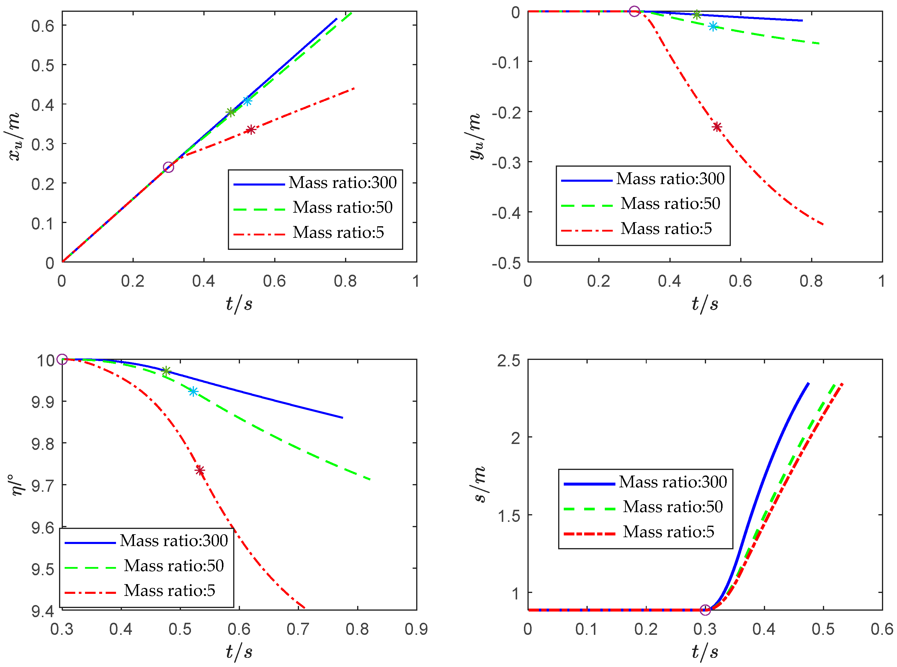
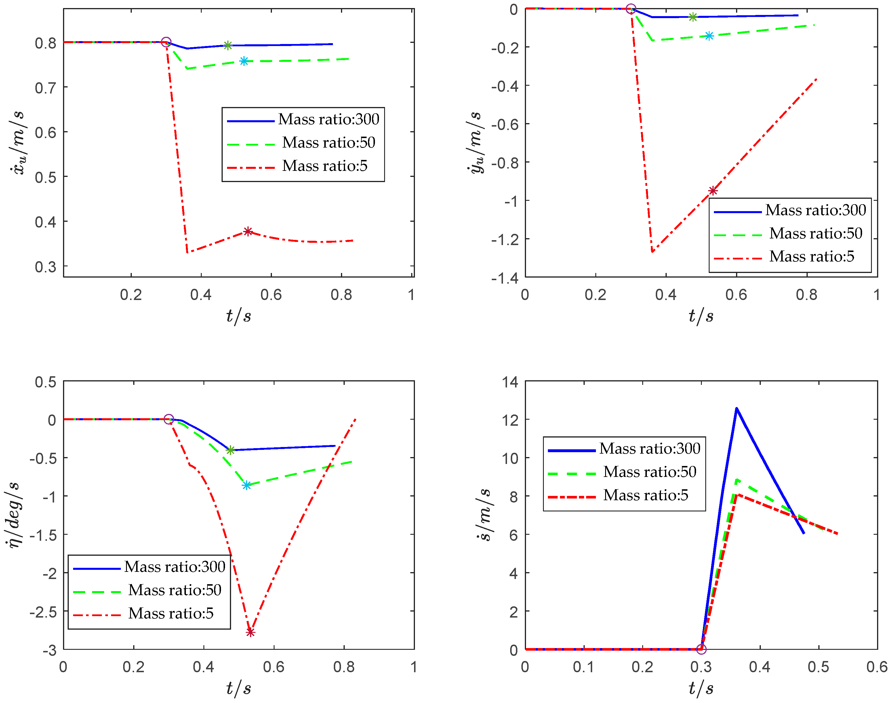
• Through numerical simulation experiments, it was found that when the mass ratio of UUV to TMV is small, the separation of the TMV will have a significant impact on the motion state of the UUV. When the TMV has completely exited the UUV, the UUV cannot automatically return to the initial cruising state, so in order to keep the UUV in a stable motion state before and after the separation of the TMV, it is necessary to study the two rigid bodies’ coupling dynamics during the process of theTMV separating from the UUV.
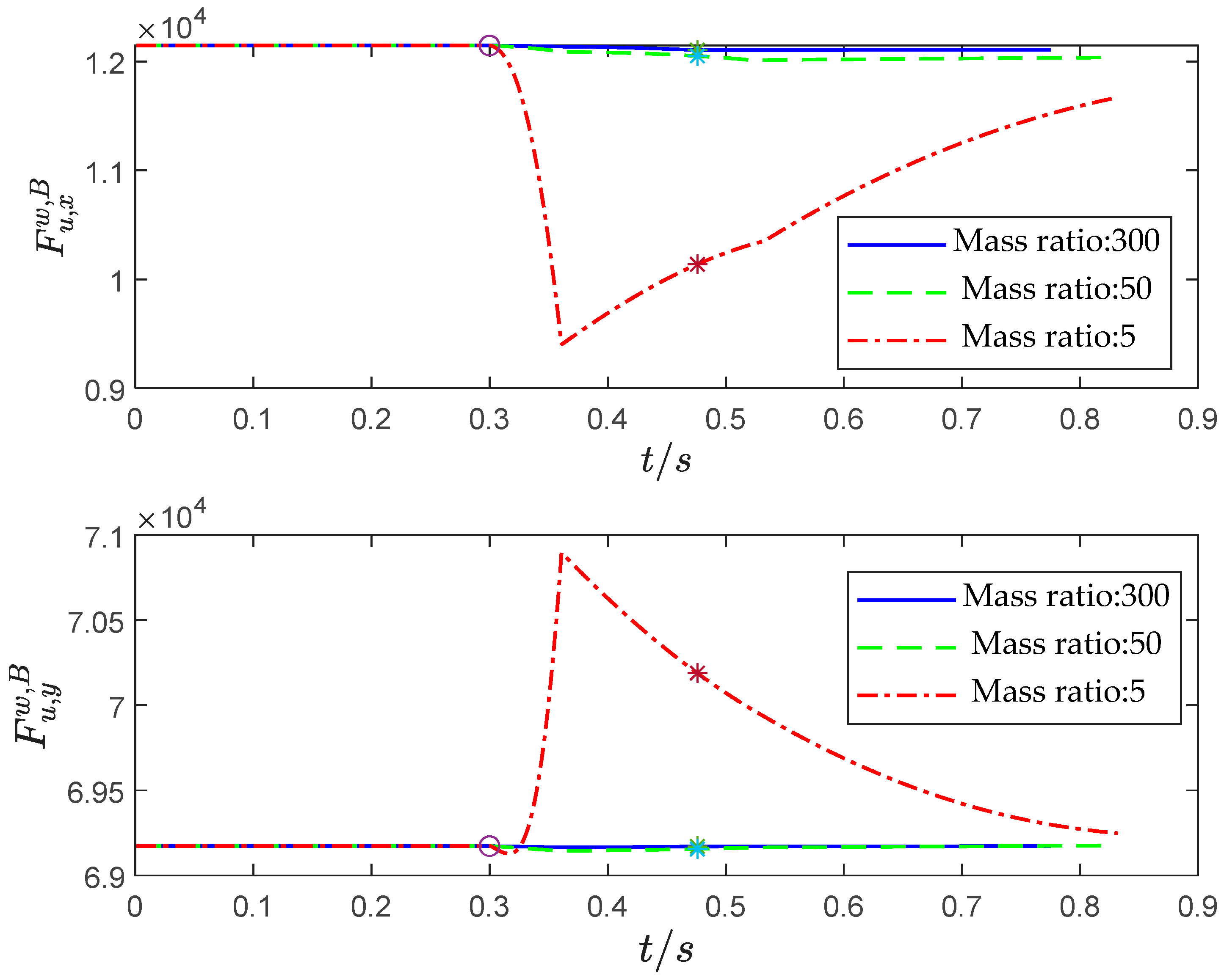
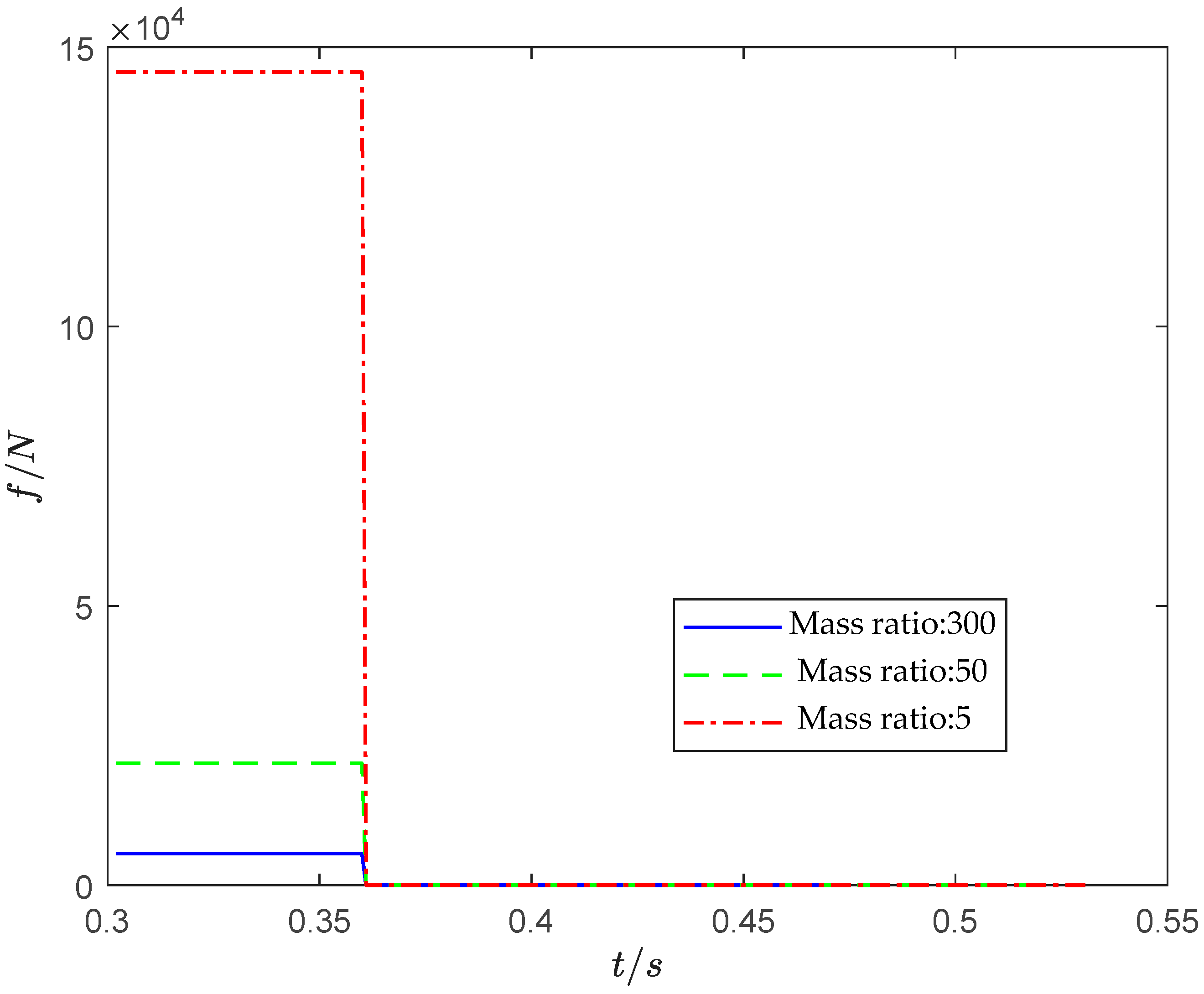
• When the TMV separates from the UUV in deep water, as the separation depth increases, the “water pressure” on the TMV’s exit section increases, so the separation resistance of the TMV increases. When the separation propulsion force parameters and other initial simulation conditions are the same, the greater the separation depth of TMV, the more severe the impact on the UUV’s motion state. In the case where the mass ratio of the UUV and TMV system is different and the terminal velocity of the TMV is basically the same, the system with a larger mass ratio consumes much less impulse during the separation process than the system with a smaller mass ratio. At the same time, when the system has a larger mass ratio, the entire separation process takes less time. That is, when the mass ratio is low, the coupling effect of the TMV on the UUV is greater.
• When a TMV separates from a UUV underwater, it is often necessary for the TMV to have a large terminal velocity, so that it can fly out of the water’s surface relying on inertia. At the same time, it is also required that the impact on the UUV’s motion state during this process is small. Therefore, the separation strategy we can adopt is to increase the mass ratio of the UUV and TMV, reduce the separation depth of the TMV, or increase the impulse acting on the TMV during the separation process.

5. Conclusions

In this paper, the coupling dynamics of the two rigid bodies of a UUV-TMV in the separation process were studied. The process of a TMV separating from a UUV was divided into the UUV constant-velocity navigation stage and the TMV separation stage. The coupling dynamics model of the two rigid bodies in these two stages was established. A large number of CFD simulation experiments were also carried out, and a precision hydraulic force calculation formula was fitted for the UUV and TMV, which improves the accuracy and reliability of the dynamics solution of the underwater separation process of the UUV and TMV. Numerical simulation experiments were carried out on the coupling dynamics of the UUV and TMV, and the coupling relationship between the motion state of the UUV and TMV during the separation of the TMV was explored. At the same time, it was also found that when the mass of the UUV and TMV is relatively small and the separation depth is great, the separation of the TMV will lead to a large change in the force acting on the UUV, so that the motion state of the UUV will be greatly disturbed. Although the separation duration of the TMV is short, the position and attitude impact on the UUV after TMV separation will last for a long time, threatening its navigational safety. The dynamics model of the separation stage established in this paper provides a more accurate mathematical model for the separation stage of the UUV and TMV. It provides a mathematical model basis for studying the stability control of a UUV during or after TMV separation from the UUV.

References

1. Sun, Y.; Pan, X.; Wang, X.; Ye, J.; Yin, X.; Dai, D. Research on unmanned underwater vehicle technology development and combat application. Ship Sci. Technol. 2023, 45, 104–109. [Google Scholar]
2. Weiland, C.J.; Vlachos, P.P.; Yagla, J.J. Concept analysis and laboratory observations on a water piercing missile launcher. Ocean Eng. 2010, 37, 959–965. [Google Scholar] [CrossRef]
3. Pan, G.; Shi, Y.; Wang, P.; Du, X. Study on the Control Law for Water Trajectory of Unpowered Carrier Under Wave Force. In Proceedings of the 3rd International Conference on Frontiers of Manufacturing Science and Measuring Technology (ICFMM 2013), Lijiang, China, 30–31 July 2013; pp. 525–530. [Google Scholar]
4. Liu, Y.; Ma, Z. The Research on Trajectory and Hot Separation of a Vertical Submarine Launched Missile. Ship Eng. 2005, 27, 6–9. [Google Scholar]
5. Liu, Y.; Zhang, Y.; Hu, D. Simulation on Capsule’s Trajectory Control of Submarine Launched Missile and Stability Studies of Capsule Moving Near the Free Surface. J. Proj. Rocket. Missiles Guid. 2005, 3, 190–191+197. [Google Scholar]
6. Li, J.; Lu, C.; Chen, X.; Cao, J. Analysis on Influence of Attached Cavity on the Trajectory of Submarine Launched Missile. J. Ballist. 2014, 26, 54–58. [Google Scholar]
7. Jiang, B.; Liu, Y.; Wang, C.; Liu, B. The Modeling and Research on Underwater Motion of Submarine Vertical Launched Cruise Missile. Tactical Missile Technol. 2013, 3, 30–34. [Google Scholar] [CrossRef]
8. Li, D.; Zhang, Y.; Dang, J.; Luo, K. Numerical Solution for Outlet Attitude of the Missile Vertical Launched from a Submarine. J. Proj. Rocket. Missiles Guid. 2009, 29, 171–173+178. [Google Scholar]
9. Shang, S.-C.; Sun, J.-Z. Research on the Affection of the Underwater Missile Launching Process. In Proceedings of the 3rd International Conference on Mechanical and Electronics Engineering (ICMEE 2011), Hefei, China, 23–25 September 2011; pp. 2594–2599. [Google Scholar]
10. Wang, Y.; Lin, T.; Jiang, H. Numerical Analysis for Water-Exit Trajectory of Submarine-launched UUV. In Proceedings of the 2018 International Conference on Mathematics, Modelling, Simulation and Algorithms (MMSA 2018), Chengdu, China, 25–26 March 2018. [Google Scholar]
11. You, T.; Wang, C.; Cao, W.; Wei, Y.; Zhang, J. Dynamic Analysis of Underwater Launched Vehicle During Water Exit. Adv. Sci. Lett. 2011, 4, 2907–2910. [Google Scholar] [CrossRef]
12. Zahid, M.Z.; Nadeem, M.; Ismail, M. Numerical Study of Submarine Launched Underwater Vehicle. In Proceedings of the 17th International Bhurban Conference on Applied Sciences and Technology (IBCAST), Islamabad, Pakistan, 14–18 January 2020; pp. 472–476. [Google Scholar]
13. Zhang, D.; Wang, C.; Shen, Y.; Wei, Y.; Xu, H. Dynamic modeling and motion prediction of two projectiles launched successively underwater. Ocean Eng. 2024, 292, 116551. [Google Scholar] [CrossRef]
14. Cheng, Y.s.; Liu, H. A Coupling Model of Water Flows and Gas Flows in Exhausted Gas Bubble on Missile Launched Underwater. J. Hydrodyn. 2007, 19, 403–411. [Google Scholar] [CrossRef]
15. Hu, K.; Ding, F. Simulation research of submarine ballistic missile launching movement modeling and manoeuvre control. Ship Sci. Technol. 2013, 35, 109–114. [Google Scholar]
16. Tan, D. Modeling and Simulation for Underwater Trajectory of the Submarine Horizontal Launched Vehicle on the Condition of Ignition Failure. J. Ordnance Equip. Eng. 2018, 39, 16–20. [Google Scholar]
17. Bian, X.; Zhao, X.; Zhu, C.; Li, X. Study on the Influence of Launch Parameters on the Safety of Vehicle Trajectory. J. Ordnance Equip. Eng. 2017, 38, 40–45. [Google Scholar]
18. Lv, B.; Huang, B.; Peng, L. Research on the uncertain factors to the control of submarine during missile launching process. Ship Sci. Technol. 2017, 39, 185–189+193. [Google Scholar]
19. Liu, B.; Luo, Y.; Li, F. Correlation Analysis on the Ejecting Velocity of Submarine-launched Missile. Ordnance Ind. Autom. 2020, 39, 63–64+78. [Google Scholar]
20. Li, J. Navigation Safety Analysis of Submarine after Underwater Vehicle Launching. Master’s Thesis, Harbin Engineering University, Harbin, China, 2022. [Google Scholar]
Figure 1. Schematic diagram of UUV and TMV.
Drones 08 00533 g001
Figure 2. The hydrodynamic drag and lift curves of UUV calculated by CFD and least squares fitting.
Drones 08 00533 g002
Figure 3. The hydrodynamic drag and lift curves of TMV calculated by CFD.
Drones 08 00533 g003
Figure 4. Static pressure distribution of the surface under a certain angle of attack of UUV.
Drones 08 00533 g004
Figure 5. Static pressure distribution of the surface under a certain angle of attack of TMV.
Drones 08 00533 g005
Figure 6. Simulation block diagram.
Drones 08 00533 g006
Figure 7. Centroid position coordinates and pitching angle of UUV, and the variation curve of sliding distance along the separation tube axis of TMV.
Drones 08 00533 g007
Figure 8. Variation curves of UUV motion velocity, pitching angular velocity, and separation velocity of TMV.
Drones 08 00533 g008
Figure 9. Variation curves of hydraulic force components in B coordinate system on UUV.
Drones 08 00533 g009
Figure 10. Separation propulsion force variation curve on TMV.
Drones 08 00533 g010
Figure 11. Variation of the separation impulse J h experienced by TMV.
Drones 08 00533 g011
Figure 12. Variation of Δ η and t L in UUV and TMV separation stage.
Drones 08 00533 g012
Figure 13. Percentage change of UUV and TMV simulation results.
Drones 08 00533 g013
Figure 14. Variation curves of hydraulic force components in C coordinate system on TMV.
Drones 08 00533 g014