Abstract
The game of pursuit–evasion has always been a popular research subject in the field of Unmanned Aerial Vehicles (UAVs). Current evasion decision making based on reinforcement learning is generally trained only for specific pursuers, and it has limited performance for evading unknown pursuers and exhibits poor generalizability. To enhance the ability of an evasion policy learned by reinforcement learning (RL) to evade unknown pursuers, this paper proposes a pursuit UAV attitude estimation and pursuit strategy identification method and a Model Reference Policy Adaptation (MRPA) algorithm. Firstly, this paper constructs a Markov decision model for the pursuit–evasion game of UAVs that includes the pursuer’s attitude and trains an evasion policy for a specific pursuit strategy using the Soft Actor–Critic (SAC) algorithm. Secondly, this paper establishes a novel relative motion model of UAVs in pursuit–evasion games under the assumption that proportional guidance is used as the pursuit strategy, based on which the pursuit UAV attitude estimation and pursuit strategy identification algorithm is proposed to provide adequate information for decision making and policy adaptation. Furthermore, a Model Reference Policy Adaptation (MRPA) algorithm is presented to improve the generalizability of the evasion policy trained by RL in certain environments. Finally, various numerical simulations imply the precision of pursuit UAV attitude estimation and the accuracy of pursuit strategy identification. Also, the ablation experiment verifies that the MRPA algorithm can effectively enhance the performance of the evasion policy to deal with unknown pursuers.
1. Introduction
The pursuit–evasion game is a classic problem in the UAV field [1], with common approaches including differential game theory [2,3] and optimal control [4,5,6]. Ref. [7] explores the feasibility of evading incoming missiles at low altitudes using a typical action library method, while Ref. [8] studies evasion strategies through trajectory planning methods. In recent years, deep reinforcement learning algorithms, represented by Deep Deterministic Policy Gradient(DDPG) [9], Proximal Policy Optimization(PPO) [10], SAC [11], and their improvements [12,13] have achieved outstanding success in fields such as robot control [14,15] and UAV navigation [16,17]. With the development of self-play technologies [18,19], reinforcement learning algorithms have also demonstrated high performance in competitive tasks [20,21]. Deep reinforcement learning can address sequential decision making problems in complex and high-dynamic scenarios, which is characteristic of pursuit–evasion games. Ref. [22] uses the TD3 algorithm to directly generate control commands for the aircraft’s control surfaces for maneuvering evasion decisions. Ref. [23] implements mixed discrete and continuous action evasion decision making through an improved SAC algorithm. Ref. [24] employs hierarchical reinforcement learning based on the PPO algorithm to enhance the robustness of evasion strategies while considering indicators such as energy consumption. Ref. [25] proposes a curriculum learning architecture that enables reinforcement learning algorithms to quickly learn effective evasion strategies and adapt to complex situations with multiple pursuers. These methods all assume that all information about the pursuer is known, including its flight attitude and pursuit strategy. However, in practical application scenarios, the uncertainty of this information, especially the pursuit strategy and the parameters of the missile, makes it difficult to apply the aforementioned methods.
In practical scenarios, an evader can detect information such as the relative position of a pursuer through sensors, but the attitude of a pursuer is usually not effectively detectable. Moreover, the pursuit strategy and parameters of the pursuer cannot be obtained in advance. In pursuit games, the pursuer usually adopts some specific strategy to approach the evader, among which proportional guidance is a common pursuit strategy. To provide more comprehensive information, many scholars have made numerous attempts in the field of aircraft attitude estimation and identification [4,5,26,27,28,29,30,31]. Ref. [27] discriminated the guidance laws of missiles by classifying the motion trajectories of missiles. Ref. [4] constructed a classifier to identify different guidance laws in real time using Bayesian inference. Ref. [28] was the first to use an interactive multiple model filter to identify the guidance law parameters of the missiles. Ref. [29] used an interactive multiple model identifier to simultaneously identify the guidance laws parameters and estimate the attitude of the pursuer. Ref. [30] proposed a multi-model mechanism to identify the guidance laws using an LSTM network through deep learning methods. Ref. [5] provided an analytical method for identifying guidance laws by analyzing the proportional guidance law. These studies have to some extent solved the problem of missing decision information, but they all consume a large amount of computational power, and the estimation accuracy of continuously changing guidance law parameters is also insufficient.
For reinforcement learning, the challenges stemming from incomplete information are twofold. First, the lack of the pursuit UAV’s flight attitude information means that the decision making problem for the evader does not possess the Markov property, making it difficult to train reinforcement learning algorithms. This issue can be resolved by providing complete information during training. In practical operational contexts, the attitude of the pursuer can be furnished by specialized estimators, and the impact of estimation errors on performance can be mitigated by robust reinforcement learning algorithms. Research in this domain has reached a considerable level of maturity, with common approaches encompassing zero-shot generalization [32,33], data augmentation [34,35], and world modeling techniques [36].
The second challenge arises from the unknown pursuit strategy. Reinforcement learning training is contingent upon the environment [37], and specific pursuit strategies and their parameters are integral components of this environment. During the algorithm’s training phase, due to the inability to predict pursuit strategy and parameters, it is necessary to assume that the pursuer uses a certain policy (such as pure proportional guidance) to construct an appropriate environment for training to obtain the optimal evasion strategy. In actual use, it is almost impossible for the pursuer to have the same pursuit strategy as the one in the training environment, leading to a significant discrepancy between the training and operational environments. This can result in the reinforcement learning algorithm making decisions that do not lead to the correct state transitions for the system in a given state [38]. Due to the properties of Markov decision processes, reinforcement learning algorithms focus solely on making the best decisions in the current state without concern for the effectiveness of previous decisions [39]. This can cause the aircraft to increasingly deviate from the originally optimal evasion route, significantly impacting the decision making performance.
To address the problems of state information deficiency and performance loss of the reinforcement learning algorithms due to the unknown parameters such as the pursuit UAV’s attitude and pursuit strategy, this paper proposes a reinforcement learning strategy adaptation algorithm based on the estimation and identification of unknown pursuer quantities and pursuit. We constructed an effective reward function that guides the evader to maneuver to the greatest extent to deplete the energy of the pursuer, thereby training a strategy to evade the pursuit UAV by controlling the evasive UAV’s lateral and longitudinal overloads. In addition, we built a new three-degree-of-freedom motion model of UAVs in a pursuit–evasion game by decomposing the relative motion of the pursuer and the evader in the horizontal plane and the vertical plane and estimated unknown quantities such as the pursuer’s velocity, acceleration, pitch angle, and heading angle through the analysis of this model. For pursuers using pure proportional guidance as a pursuit strategy, we derived the identification model of the proportional guidance constant and eliminated the zero-crossing error in the identification results through the Kalman filtering algorithm. Based on the identification of the proportional guidance constant, we represented the relationship between the relative motion situation of evader and pursuer UAVs and evaders’ lateral overload and side overload as an affine dynamic system. On the basis of the reinforcement learning decision instructions and the identification results of the proportional guidance constant, we provided an action compensation equation through this system. Solving this equation yields the optimal decision correction for existing reinforcement learning strategies against an unknown pursuer. Unlike the method of adding noise during the training process to improve the robustness of reinforcement learning algorithms, the action compensation algorithm proposed in this paper theoretically ensures the effectiveness of the optimal strategy against a pursuer with different pursuit strategy parameters.
This paper is organized as follows: Section 2 provides the process of addressing the evasive decision making problem using reinforcement learning. Section 3 introduces the relative motion model of UAVs in pursuit–evasion games and outlines the methods for estimating the unknown quantities and pursuit strategy of the pursuer. Section 4 presents a Model Reference Policy Adaptive (MRPA) algorithm. Section 5 comprises the experimental segment, wherein the algorithms proposed in Section 2, Section 3 and Section 4 are subjected to numerical simulation for empirical validation. Conclusive remarks and a summary of our findings are presented in Section 6.
2. SAC for Evasive Decision
2.1. Problem Formulation
In pursuit–evasion games, the evader agent provides decision commands based on the relative dynamic situation between the pursuer and the evader, controlling the aircraft’s maneuvers. The pursuer tracks the evader according to a specific pursuit strategy. In this process, the control of the aircraft still follows the OODA loop. The observation and orientation (OO) phase of the OODA loop in the pursuit–evasion game, which involves state observation and processing as well as the estimation of unknowns, will be discussed in Section 3.3. We assume that the agent can always obtain fully processed complete situational information. DA generates control commands for the aircraft and executes them, with this part handled by the agent. The agent’s decisions directly impact the aircraft’s survivability.
This paper constructs a Markov decision process (MDP) model for the pursuit–evasion game based on a three-degree-of-freedom dynamic model, which can be described by the tuple , where represents the state space and represents the action space; both are continuous spaces over the real numbers. During the training process, each component of the actions and states is normalized to the range [0, 1]. denotes the state transition model; in air combat decision making problems, both the evader and pursuer follow specific motion laws; hence, can be represented by a deterministic system. signifies the system’s reward, which is a function of the state and action, with serving as the discount factor.
2.2. State Space
In the game of pursuit–evasion, the agent needs to make decisions based on the relative position of the aircraft and the pursuer, as well as the flight attitudes of both. Therefore, the state space is composed of three parts: the attitudes of the evasive and pursuit UAVs and the relative position between the evasive and pursuit UAVs. In the three-degree-of-freedom model, the attitudes of evasive and pursuit UAVs are described by the velocity yaw angle and velocity pitch angle . The relative position between the evasive and pursuit UAVs is characterized by the line-of-sight yaw angle , line-of-sight pitch angle , and relative distance R. To ensure the Markov property of the system, the state space also incorporates the derivatives of the line-of-sight yaw angle , the line-of-sight pitch angle , and the relative distance . Thus, the state is represented as:
2.3. Action Space
The agent provides control signals to the aircraft through decision making commands. In a three-degree-of-freedom model, the aircraft’s attitude is controlled by the velocity yaw angle and the velocity pitch angle. By controlling the aircraft’s attitude and velocity magnitude, the flight state can be managed. The rate of change of the velocity magnitude, as well as the yaw and pitch angles, can be represented as longitudinal, lateral, and axial overloads. Therefore, the action space is set as
2.4. Transition Function
Both the evasive and pursuit UAVs are simulated using a three-degree-of-freedom model, neglecting the roll angle and describing the attitudes of the evasive and pursuit UAVs solely through the yaw and pitch angles. Discretizing the three-degree-of-freedom model based on the previously defined states and actions yields the transition equations as follows:
where is the time step and represent the components of the distance between the evasive and pursuit UAVs in the north–east–down (NED) coordinate system.
2.5. Reward Function
To enable the evader to survive for as long as possible under the pursuer’s pursuit during training, the reward function is divided into sparse rewards and real-time rewards. Sparse rewards are based on survival time: at the final state, when the survival time exceeds 24 s, the evader receives a reward of 100; when it exceeds 27 s, it receives a reward of 200; and when it exceeds 30 s, it receives a reward of 400. For every additional second of survival time, the reward increases by 50. Additionally, if the survival time is less than 24 s, for each second less, the aircraft receives a penalty of −100.
The purpose of continuous rewards based on the rate of change of the distance between the pursuer and the evader is to enable the agent to make decisions at each step that are more conducive to increasing survival time. Considering that the rate of change of pursuer-to-evader distance directly reflects the pursuer’s approach to the aircraft, an increase in the rate of change means the pursuer takes longer to catch up. An exponential function is used for adjustment to avoid obtaining lower discounted cumulative rewards when the survival time is longer. The formula for the continuous reward is ultimately expressed as:
2.6. SAC Algorithm
The Soft Actor–Critic (SAC) algorithm is a widely applied maximum-entropy reinforcement learning method. Building upon the traditional Actor–Critic (AC) framework [11], the SAC algorithm introduces the concept of entropy regularization, altering the policy optimization goal to maximize the sum of rewards and policy entropy. The introduction of policy entropy enables more effective exploration in reinforcement learning, and the adaptive adjustment of different entropy weights allows the SAC algorithm to explore better policies across various tasks. After introducing the entropy regularization term, the state value function can be written as:
in which Q represents the action value function, V represents the value function, denotes the updated step size, and indicates the entropy of the policy . Like soft Q-learning, the soft Bellman equation in SAC is given by:
In decision making within continuous spaces, the SAC algorithm employs neural networks to parameterize and approximate the behavior value function and the policy . To prevent overestimation of the action value function during training, SAC adopts the idea from Double Q-learning, utilizing two independent Q networks to estimate the action values and selecting the network with the smaller Q value for each update. The update mechanism for the Q network is similar to reinforcement learning algorithms in the AC framework like DDPG [9], with the loss function incorporating an entropy regularization term. The loss function is expressed as:
where R represents the sampled data from the replay buffer and denotes the discount factor. To ensure the stability of the policy, the SAC algorithm also introduces target networks.
The loss function of the policy network derived through Gaussian distribution reparameterization is expressed in terms of the Kullback–Leibler (KL) divergence, considering the two Q networks, as follows:
In the SAC algorithm, the entropy regularization coefficient determines the exploration of the algorithm. Different states require varying levels of exploration. When the optimal action for a state is relatively certain, the entropy should decrease, and vice versa. Therefore, the SAC algorithm also needs to consider a constrained optimization problem, which ensures that while maximizing the discounted cumulative return, the average entropy cannot be less than a threshold :
Hence, the loss function for the entropy regularization coefficient can be derived as:
3. Pursuit Strategy Parameter Identification
3.1. Relative Motion Model
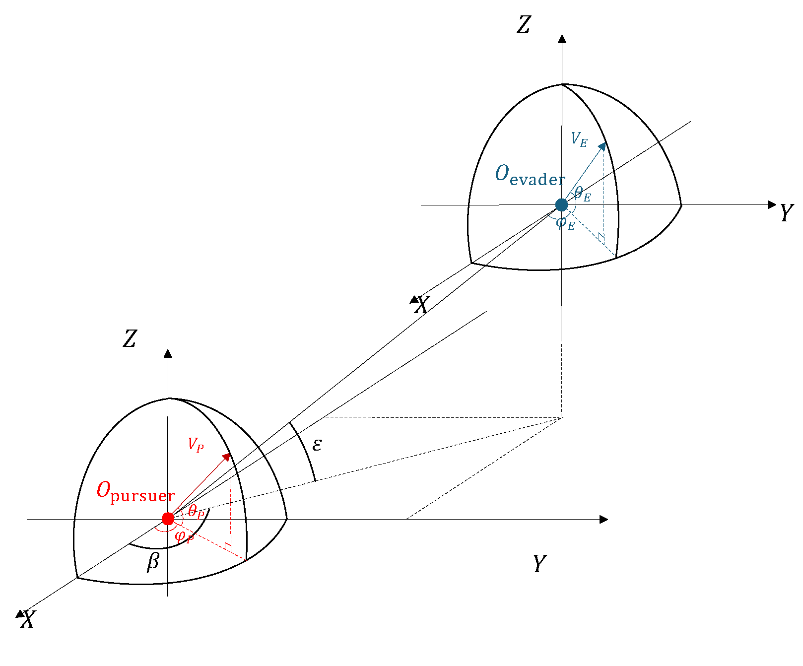
The pursuit–evasion game between the evasive and pursuit UAVs can be described in the Cartesian coordinate system, as shown in Figure 1. Without considering roll, the kinematics of the evasive and pursuit UAVs can be written as:
where represent the position in the NED (north–east–down) coordinate system, is the pitch angle, is the yaw angle, the subscript E denotes the evader, and the subscript P denotes the pursuer. The rate of change of the evader’s velocity magnitude is determined by factors such as engine thrust and aerodynamic drag, which do not affect the subsequent analysis. The direction of the UAV’s velocity, i.e., yaw angle and pitch angle, is controlled by the lateral acceleration and longitudinal acceleration . Then, we can obtain:
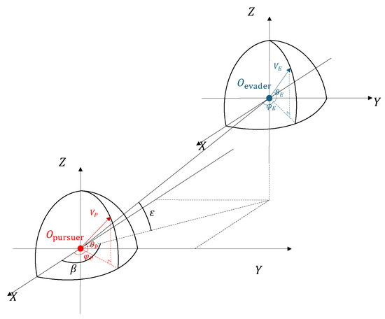
Figure 1.
Relative motion relationship between evasive and pursuit UAVs.
The pursuer uses proportional guidance as a pursuit strategy, which indicates that the angular velocities of the pursuer’s pitch and yaw angles are proportional to the yaw and pitch angular velocities of the line of sight (LOS), as follows:
where are proportional navigation constants and the calculations for yaw angle and pitch angle of the line of sight (LOS) are the same as in Equation (3).
By decomposing the motion of evasive and pursuit UAVs within horizontal and vertical planes, we can derive a new relative motion model:
This model describes the relative motion between the evasive and pursuit UAVs through their attitudes, avoiding the use of position coordinates. This reduces the complexity of the analysis and the dependence on observational information.
3.2. Estimation of Uncertainty and Disturbance Terms
In Equations (14)–(16), the terms with the subscript E represent information about the evader, which are known terms. The terms , , and describe the relative motion and are considered measurable known terms. The terms with the subscript P represent information about the pursuer, which are unknown terms. In Equations (14)–(16), the unknown terms are , , and . First, consider the estimation of and . In Equations (14)–(16) and subsequent calculations, the pursuer’s yaw angle and the line-of-sight yaw angle appear together in the form of . Therefore, is treated as a single unknown term for estimation. Separating the known and unknown terms in Equations (14)–(16) produces:
where the unknown terms and are also estimated by the following equation:
From Equation (13), it is known that identifying the proportional navigation constant requires calculating the angular velocities of the pursuer’s yaw and pitch angles. To obtain terms related to these, assuming and denoting , differentiating Equations (14)–(16) produces:
Upon observing , it can be found that the three unknown terms can be expressed as a linear combination of the rate of change of the pursuer’s velocity, the yaw angle, and the pitch angle’s angular velocities. With , we have:
where can be expressed as:
The estimation method for and has already been provided in Equations (19) and (20); hence, it is only necessary to determine the unknown term to obtain the angular velocities of the velocity yaw angle and the velocity pitch angle. The terms on the left side of Equations (30)–(32) can be obtained by numerical differentiation of observable values, with being the known terms, and theoretically, can be directly subtracted. Considering the noise included in the observation and the potential errors caused by numerical differentiation, this paper introduces a first-order low-pass filter G to process . Taking as an example, the estimated value of is , which can be represented as:
The transfer function filter G is:
where represents the time constant of the filter. By substituting Equation (30) into Equation (37) and performing an inverse Laplace transform, we can obtain:
It can be seen from the above equation that the estimation of no longer depends on the second-order differentiation of the observed values. The first-order low-pass filter G not only processes the observational noise but also avoids additional differentiation operations, thereby preventing errors introduced by numerical differentiation. The estimator constructed by Equations (40), (42), and (44) relies solely on the observable quantities: LOS (line-of-sight) pitch angle, yaw angle, the range between the evasive and pursuit UAVs, and their respective rates of change. Each estimator depends on only one parameter, . Once the three unknowns are obtained from the estimator, the pursuer’s pitch rate, yaw rate, and velocity change rate can be calculated according to Equation (33).
3.3. Guidance Law Parameter Identification
The proportional navigation law indicates that the angular velocities of the pursuer’s yaw and pitch angles are proportional to the angular velocities of the line-of-sight yaw and pitch angles, with the proportionality constant being the proportional navigation constant, which are observable values. Therefore, the pursuer’s proportional navigation constant can be calculated by the following formula:
It is observed that Equations (46) and (47) include operations involving the division by angular velocity. In theory, the angular velocity of the line-of-sight yaw angle and the angular velocity of the pursuer’s velocity yaw angle should both be zero simultaneously, and the angular velocity of the line-of-sight pitch angle and the angular velocity of the pursuer’s velocity pitch angle should also both be zero simultaneously, thus avoiding singularity issues. However, in actual identification processes, due to the presence of estimation and observation errors, these quantities usually do not simultaneously equal zero. When the denominator is zero and the numerator does not equal zero due to error, this error can be greatly magnified, leading to a significant estimation error in the proportional navigation constant, known as the zero-crossing error.
The proportional navigation constant K simultaneously controls the relationship between the velocity pitch angle and the line-of-sight pitch angle, as well as the velocity yaw angle and the line-of-sight yaw angle. Therefore, Equations (46) and (47) provide two independent estimates of K. Under normal circumstances, the rates of change of the velocity yaw angle and pitch angle will not both be zero at the same time, so the zero-crossing error will not occur simultaneously in both estimates. Even if the zero-crossing error occurs in both estimates at similar times, historical estimates are still reliable. Based on the above analysis, this paper introduces a Kalman filter to deal with the zero-crossing error. The main formulas of the Kalman filter are:
where represents state covariance and represents process noise covariance. Assuming K is a constant and is the observation of K, then,
The covariance of the observation noise is defined as
where is a threshold; when the absolute value of the angular velocity of the velocity yaw or pitch angle is less than this threshold, the observation variance increases, controlled by the parameter R, while the parameter a determines the rate of change of the variance near the threshold. Since the zero-crossing error is caused by the angular velocity of the velocity yaw or pitch angle in the denominator being equal to or too close to zero, in the Kalman filter, when one of the angular velocities of the velocity yaw or pitch angle is very close to zero, the measurement variance of the corresponding K estimate in the filter will be amplified. The filter will consider this estimate unreliable and thus trust the other estimate. If both estimates are unreliable, the filter will trust the historical values.
4. Model Reference Policy Adaptation Algorithm
This section discusses the principle behind the failure of reinforcement learning evasion strategies when facing an unknown pursuer that differs from the training environment. Building on this, and based on the relative motion model and the affine dynamics model discussed in this paper, an action compensation scheme is proposed, aiming to reduce the loss of strategic performance when facing different pursuers.
4.1. Problem Formulation
Whether it is value function-based reinforcement learning algorithms or direct policy search-based reinforcement learning algorithms, their goal is to find the optimal policy in a specific environment. The Bellman equation and the policy gradient theorem shown in Equations (55) and (56) indicate that the optimal policy is related to the environment [40].
In these equations, represents policy, and p denotes the state transition probabilities of the environment, with different environments having distinct state transition probabilities. When the environment changes, p changes accordingly, and the originally optimal policy no longer retains its optimality. In deep reinforcement learning, the state transition probabilities of the environment are considered unknown quantities. Through continuous interaction with the environment, the policy network or value function network within the reinforcement learning model learns information about the environment’s state transition probabilities from the data and fits the action value function or optimal policy based on this information. Therefore, the optimal policy of deep reinforcement learning algorithms is still constructed based on a specific environment.
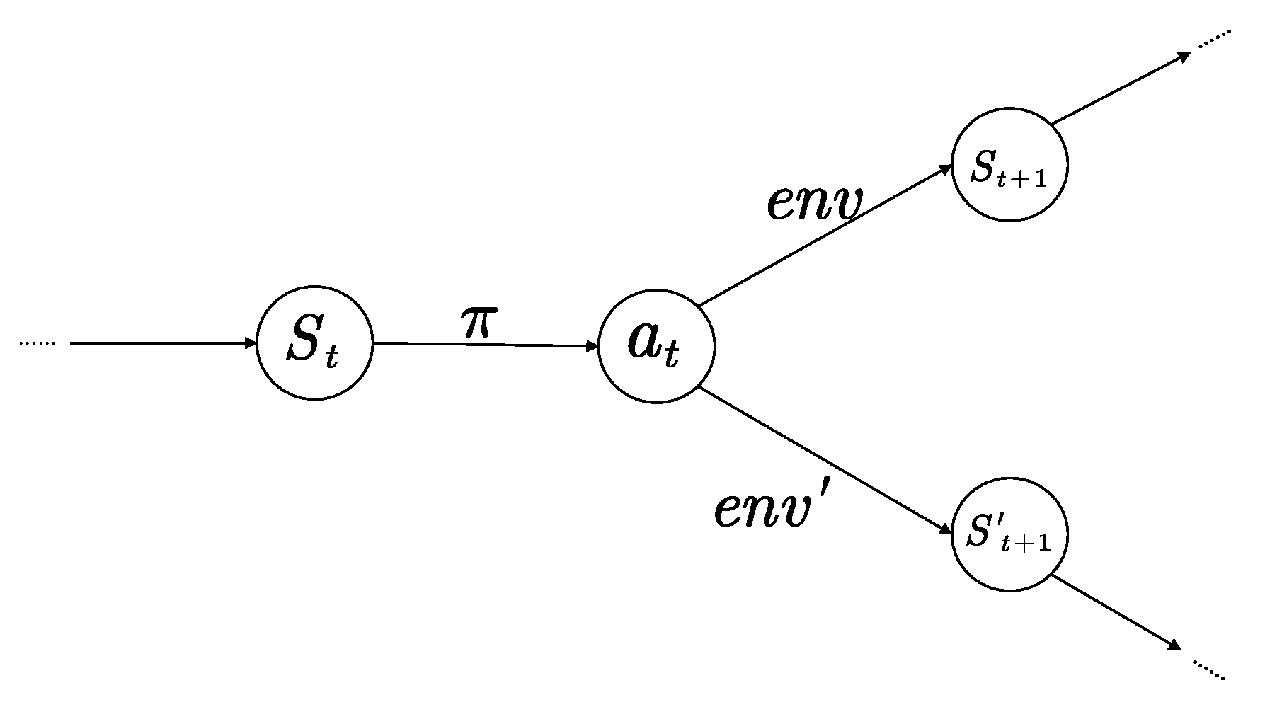
From the perspective of state transitions, the significance of the optimal policy lies in enabling the agent to choose a particular action with the highest probability in a given state and transition to the next specific state, repeating this process to ultimately form a specific trajectory with the highest expected discounted cumulative reward. When the environment changes, the process of state transitions will also change. Since the agent cannot perceive the changes in the environment, the optimal policy will cause the agent to choose the same actions as in the ideal environment but fail to transition to the specific next state. Due to the characteristics of the Markov decision process, the agent only cares about choosing the best action in the current state and does not concern itself with whether the actions chosen in the previous state achieve the desired effect. Therefore, as shown in Figure 2, incorrect state transitions will continue until the task is terminated, and the trajectory formed by the agent will gradually deviate from the expected optimal trajectory, resulting in an expected cumulative reward that is lower than the optimal value. The degree of deviation and the extent of the reduction in expected cumulative reward are related to the magnitude of the environmental change.
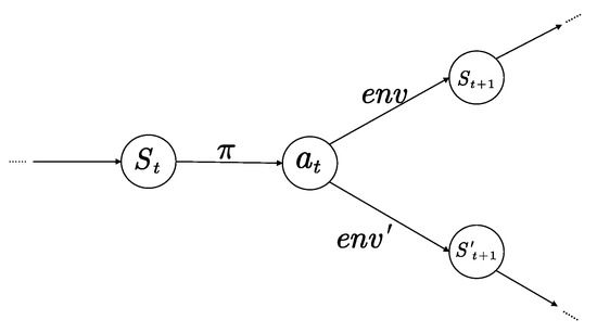
Figure 2.
Failure mechanism of optimal policy.
From the analysis above, it is known that the key to ensuring the performance of the optimal policy does not decrease after environmental changes is to enable the agent to continue operating along the original optimal trajectory in the changed environment, that is, to ensure that the agent can achieve the same state transition as in the original environment after making the optimal action in any state. To achieve this without retraining the optimal policy, it is necessary to make certain corrections to the optimal actions based on the changes in the environment.
4.2. MRPA Method
In engineering applications, adaptive control methods are commonly used to improve the control performance of a system when there is uncertainty in the model. Model reference control is one of the more popular methods. A model reference control system mainly consists of a controller, a reference model, an adaptation rate, and the controlled object [41]. The idea is to design an adaptation rate so that the deviation between the output signal of an uncertain controlled object and the output signal of the reference model with the same input is as small as possible [42].
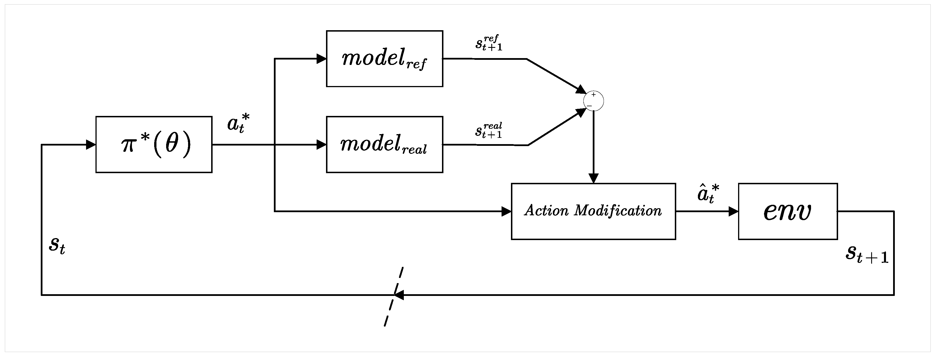
Inspired by Model Reference Adaptive Control (MRAC), this section proposes a Model Reference Policy Adaptation (MRPA) algorithm. The original environment in which the optimal policy is trained serves as the reference environment. Based on this, an adaptation rate is designed to adjust the actions selected by the optimal policy according to the difference in state transitions between the reference environment and the actual environment for a given state–action pair. This adjustment aims to eliminate the difference or make it as minimal as possible, thereby reducing the performance loss caused by environmental changes. The process of the Model Reference Policy Adaptation algorithm is shown in Figure 3.

Figure 3.
Structure of MRPA algorithm.
The reference model utilizes an affine dynamic system in the form of
In the pursuit–evasion game discussed in this paper, the state vector and action vector can be represented as
Combining the relative motion model of UAVs presented in Section 3.1 with Equations (12) and (13) yields:
and
where
Assuming , we found
Summarizing the above gives
By discretizing Equation (57), we obtain
From Equations (59) and (66), it can be inferred that is a function matrix with as the parameter. When the agent selects a certain optimal action , the state transition equation is:
In the pursuit–evasion game, when facing a pursuer different from the training environment, the parameter will change, indicating that the environment has changed. At this point, under a certain action , the state transition equation is:
To maintain consistent state transitions, even if the agent can achieve the same state transition as when selecting the optimal action in the original environment, we have:
Solving for the action that should be chosen in the altered environment yields:
Equation (72) represents the action compensation equation, where is obtained through the identification algorithm discussed in Section 3.3 and is updated in real time during the decision making process.
5. Experiments
In this section, we first provide the experimental setup and then demonstrate the training effectiveness of the SAC algorithm in the pursuit–evasion game scenario, followed by numerical simulation to verify the performance of the relative motion model, pursuit UAV’s attitude, and guidance law parameter estimation algorithms proposed in this paper, and through ablation experiments, we validate the effectiveness of the MRAC algorithm.
5.1. Experimental Settings
During the training process of the evasive policy using the SAC algorithm, to simulate pursuers approaching from different directions and distances, we set a uniform distribution for the initial velocity direction of the pursuer and the initial position of the aircraft, randomly generating different initial situations. The generation parameters for each initial state are shown in Table 1, and the hyperparameters of the SAC algorithm are shown in Table 2:

Table 1.
Initial state setting.

Table 2.
Parameters of SAC.
To test the performance of the relative motion model and the pursuit UAV’s attitude estimation and pursuit strategy identification algorithms, this paper designs two flight trajectories, the barrel roll maneuver and straight-line maneuver, to simulate and test the methods proposed in the text. The control amount for the barrel roll maneuver is:
where R represents the radius of the barrel roll maneuver, denotes the horizontal velocity, and T represents the rotation period of the barrel roll maneuver. Parameters for the first-order filter used in the pursuit UAV’s attitude estimation and the Kalman filter used in pursuit strategy estimation are shown in Table 3.

Table 3.
Parameters of filters.
In the experiments of this section, the state transition model used during the training of the reinforcement learning algorithm as well as the UAV kinematics model used in the pursuit strategy identification and evasion strategy testing both operate with a simulation time step of 1 ms. The observation cycle for the pursuer’s state estimation and pursuit strategy identification algorithm is 10 ms.
5.2. Validity of Relative Motion Model
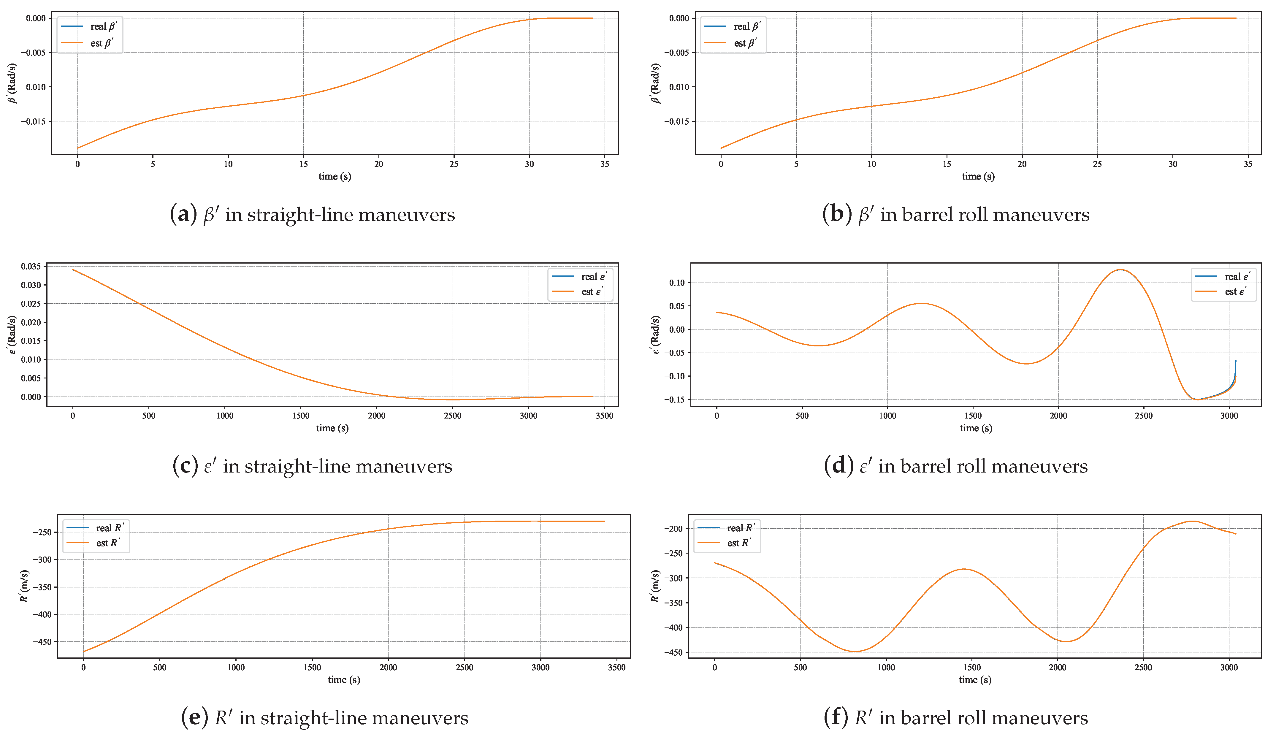
The relative motion model proposed in Section 3.1 is constructed by decomposing the motion of the pursuer and the evader in the horizontal plane and the vertical plane, and approximate methods are used during the derivation process. The experiments in this section simulate the aircraft performing barrel roll maneuvers and straight-line movements, and the effectiveness is verified by comparing the differences between the relative motion states calculated by our proposed model in the simulation and the actual states.
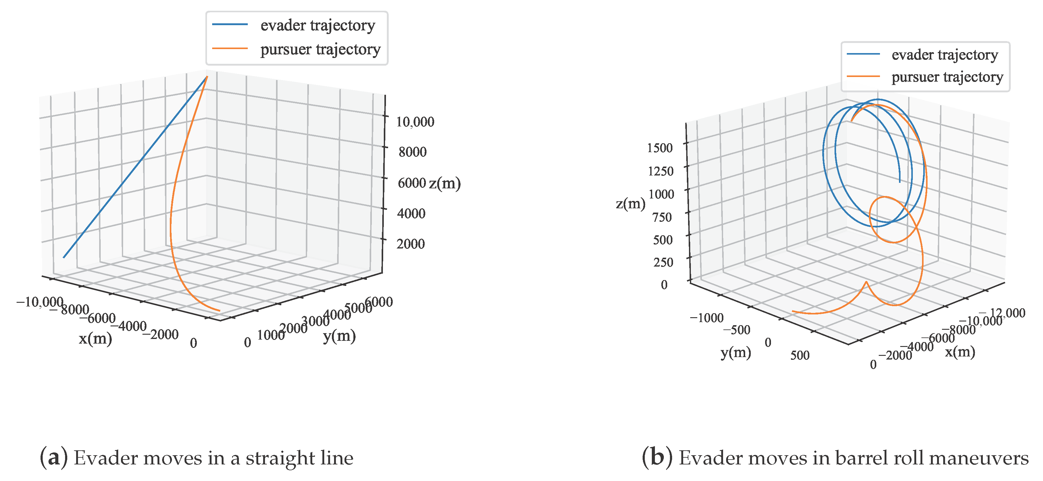
Figure 4 displays the trajectories of the pursuer and evader during straight-line maneuvers and barrel rolls of the aircraft. As shown in Figure 5, in both maneuvering modes, the relative motion situation calculated by the model proposed in this paper is almost consistent with the true value. At the end of the motion, there is some error in the calculation of R. This error is due to the approximation used in the model, where , which fails when x is not close to zero. The model uses the ratio of relative displacement to R to approximate the change in the yaw angle. As the pursuer is about to catch up with the evader, R decreases, causing some distortion in the model. Experimental results also show that this distortion only occurs about 1.88 s before the end of the simulation, and the model maintains a high degree of accuracy.
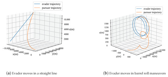
Figure 4.
Trajectories of pursuit and evasive UAVs.
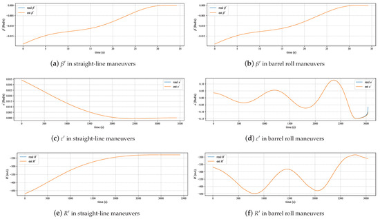
Figure 5.
Performance of relative motion mode.
5.3. Performance of Guidance Law Parameter Identification
This chapter presents the simulation results of the guidance law parameter identification. In the experiment, the velocities of the evader and pursuer used are the same as in Table 1, with the pursuer’s velocity linearly decaying. The initial position of the aircraft is [10,000, 0, 1000], and the initial pitch angle of the pursuer is , with the yaw angle being . The aircraft’s barrel roll maneuver has a period of 1 s with a horizontal velocity of 100. For the straight-line motion, the pitch angle is 1 and the yaw angle is .
To verify the adaptability of the algorithms proposed in this paper in high-dynamic environments, we conducted identification experiments on dynamically changing guidance law parameters. The variations in the proportional navigation constant include step changes, linear changes, and sinusoidal variations. The time for the step change is 8 s, the rate of change for the linearly varying proportional navigation constant is , and the period for the sinusoidal variation is .
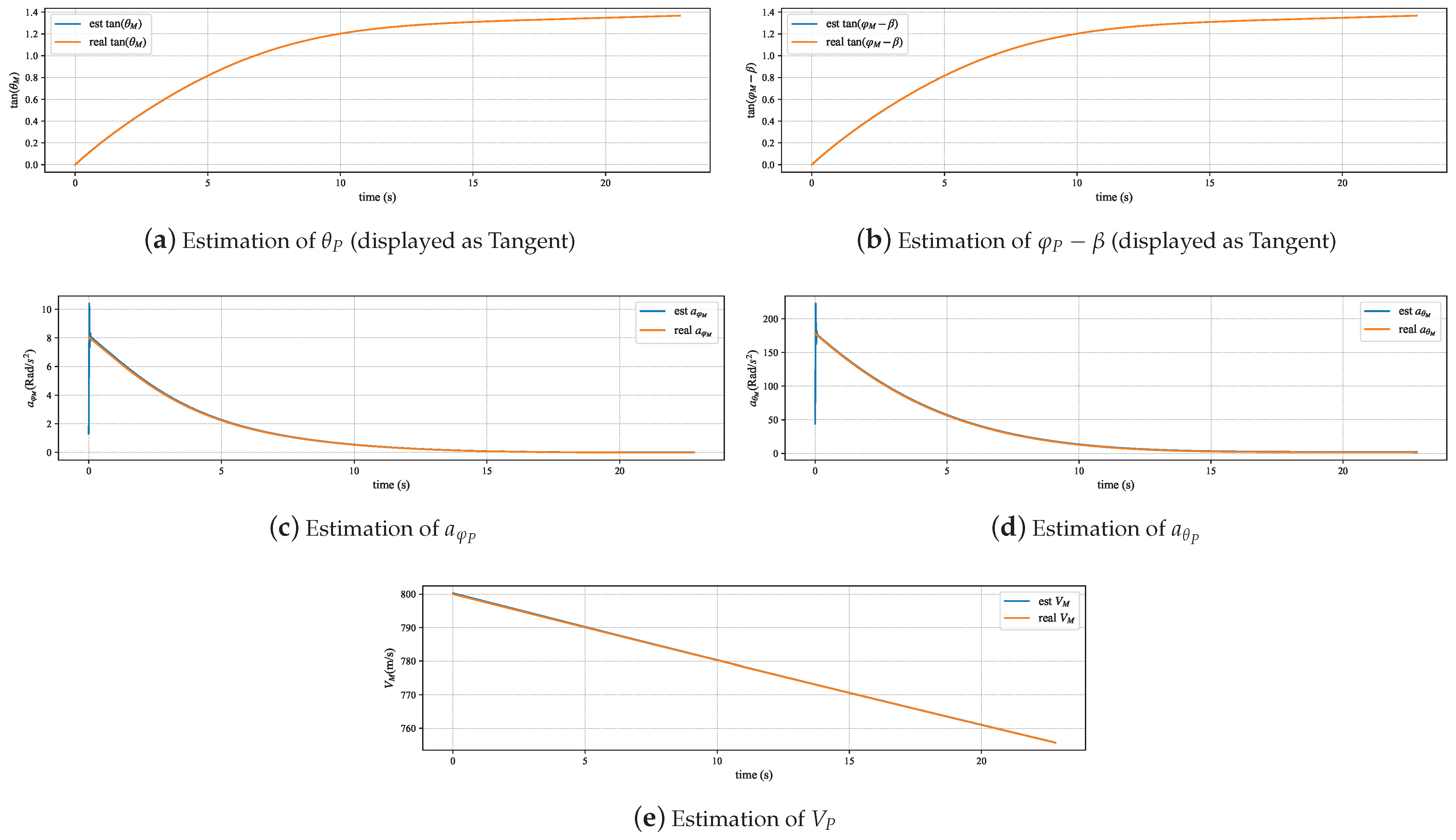
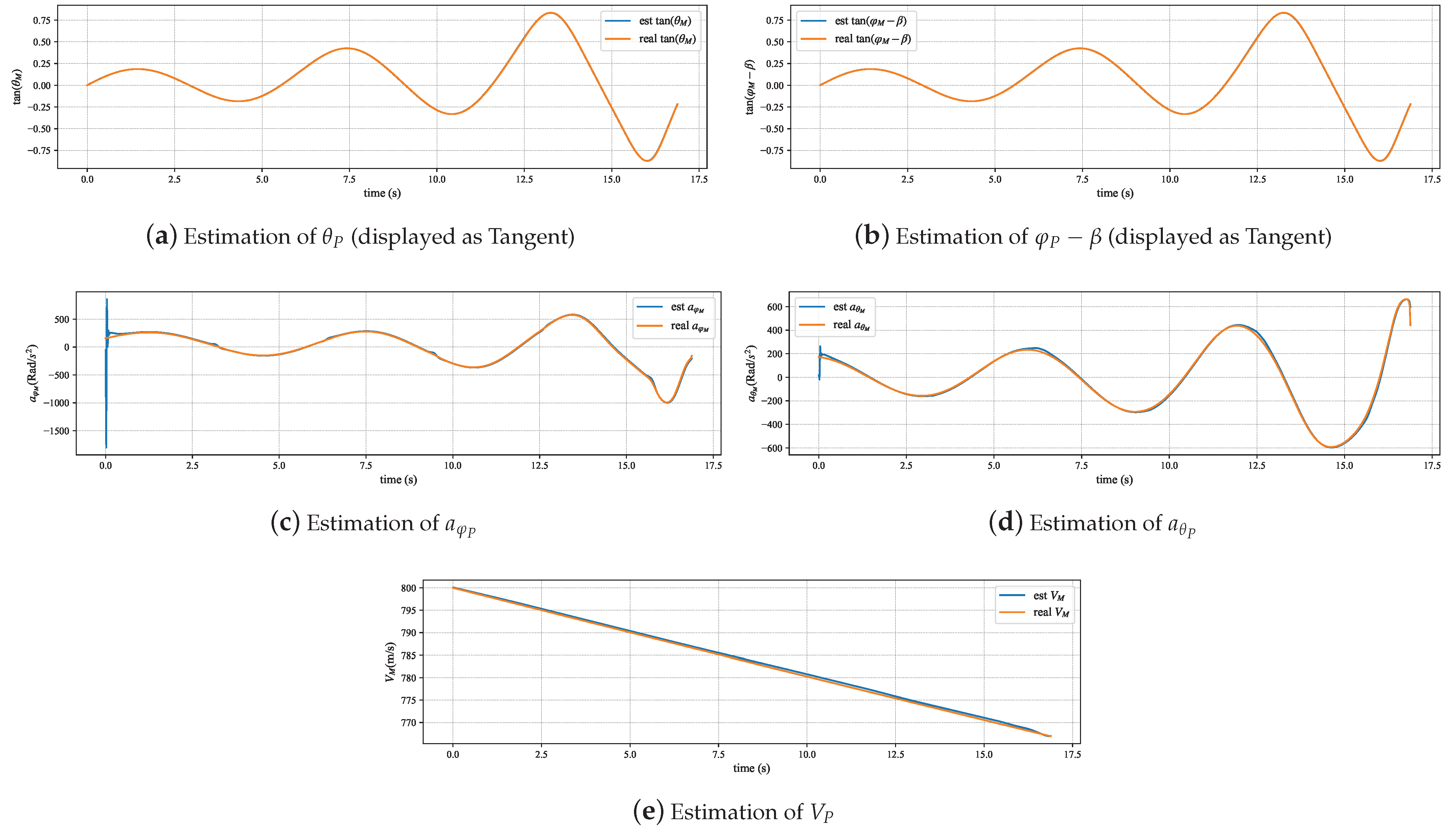
The experimental results in Figure 6 and Figure 7 indicate that the pursuer flight state estimation model can accurately and stably estimate the pursuer’s attitude, velocity, and longitudinal and lateral accelerations. There are certain errors at the beginning and end stages of the simulation process. The error at the beginning stage originates from the first-order low-pass filter used in the attitude estimation not being converged, and the error at the end stage comes from the error of the relative motion model. Figure 8 and Figure 9 demonstrate that the identification algorithm proposed in this paper has a sufficiently high degree of accuracy for the identification of constant guidance law parameters, with errors controlled within approximately 0.2, and the response time is less than 0.5 s. Figure 10, Figure 11 and Figure 12 demonstrate that the method proposed in this paper can also effectively track and identify the dynamically changing guidance law parameters. Additionally, by comparing the identification results before and after the Kalman filter in Figure 8, Figure 9, Figure 10, Figure 11 and Figure 12, it can be seen that the filter designed in this paper can effectively eliminate the interference of zero-crossing errors on the identification results.
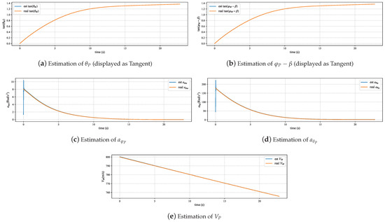
Figure 6.
State estimation in straight-line maneuvers.
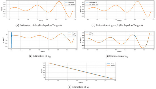
Figure 7.
State estimation in barrel roll maneuvers.

Figure 8.
Identification of K in straight-line maneuvers.

Figure 9.
Identification of K in barrel roll maneuvers.

Figure 10.
Identification of K in barrel roll maneuver with step change.

Figure 11.
Identification of K in barrel roll maneuver with linear change.

Figure 12.
Identification of K in barrel roll maneuver with sinusoidal variation.
In practical application scenarios, the observational signals provided by sensors are generally not unbiased, and the observational values obtained by the pursuit strategy identification algorithm typically contain some noise [43]. To test the performance of the pursuit strategy identification algorithm under input signals with observational noise, we conducted an additional set of tests by providing the identification algorithm with input signals containing random noise to test its robustness to noise. We tested proportional navigation parameters with step changes, linear changes, and sinusoidal changes, with the parameters for the three types of changes being the same as in previous experiments. Due to the coupling between the input signals of the pursuit strategy identification algorithm, we directly added observational noise to the observational values of the pursuer’s position coordinates and calculated the input signals in the same manner as Equation (1) to ensure the plausibility of noise in each signal. The added noise was Gaussian noise with a mean of 0 and a standard deviation of 20.
The experimental results depicted in Figure 13, Figure 14 and Figure 15 indicate that despite the noise in the input signals causing some impact on the identification results, the method proposed in this paper is still capable of stably tracking the dynamically changing proportional navigation constants. When tracking the step change in proportional navigation constants, the average error is 0.248; for the linear change, the average error is 0.249; and for the sinusoidal change, the average error is 0.217. These error levels are higher than those observed in noise-free conditions. The presence of observational noise not only directly affects the estimation but also exacerbates the negative impact of zero-crossing errors. Not only does division by zero amplify more errors, but observational noise may also increase the frequency of zero-crossing errors. Since the Kalman filter and low-pass filter included in the method proposed in this paper have certain noise suppression effects, the impact of observational noise on algorithm performance is controlled within an acceptable range.

Figure 13.
Identification of K in barrel roll maneuver with linear change and observational noise.

Figure 14.
Identification of K in barrel roll maneuver with step change and observational noise.

Figure 15.
Identification of K in barrel roll maneuver with sinusoidal variation with observational noise.
5.4. Performance of MRAC Method
This chapter begins by comparing the MRPA algorithm proposed in this paper with other methods that enhance the generalization performance of reinforcement learning to verify the superiority of the MRPA algorithm in dealing with unknown pursuers. We selected two baseline methods for comparison. The first method is the traditional generalization approach, Multi Env–SAC, which enhances the evasion strategy’s ability to cope with different pursuers by considering various pursuit strategies during the training phase. The second method is the data augmentation method, Data Argument–SAC, proposed in Reference 1, which improves the generalization performance of reinforcement learning algorithms by applying data augmentation to the state data in the experience replay buffer, and it is currently the most widely used method to enhance the generalization capabilities of reinforcement learning algorithms.
When implementing Multi Env–SAC, to enable the algorithm to learn evasion strategies against different pursuers, we added the pursuit strategy parameter K to the state information based on the SAC algorithm used in Section 2, adjusting the state space to:
with all other parts remaining unchanged and K varying within the range of [3, 6]. The data augmentation method proposed in Reference 1 provides various data augmentation techniques for reinforcement learning algorithms based on image input, such as adding noise, color changes, image cropping, and flipping. However, since the input signal of the reinforcement learning algorithm used in this paper is a state vector, only noise addition is used for data augmentation, adding Gaussian noise with a mean of 0 and a standard deviation of 0.05 to the normalized state data. Both comparative methods are trained with settings identical to the original methods.
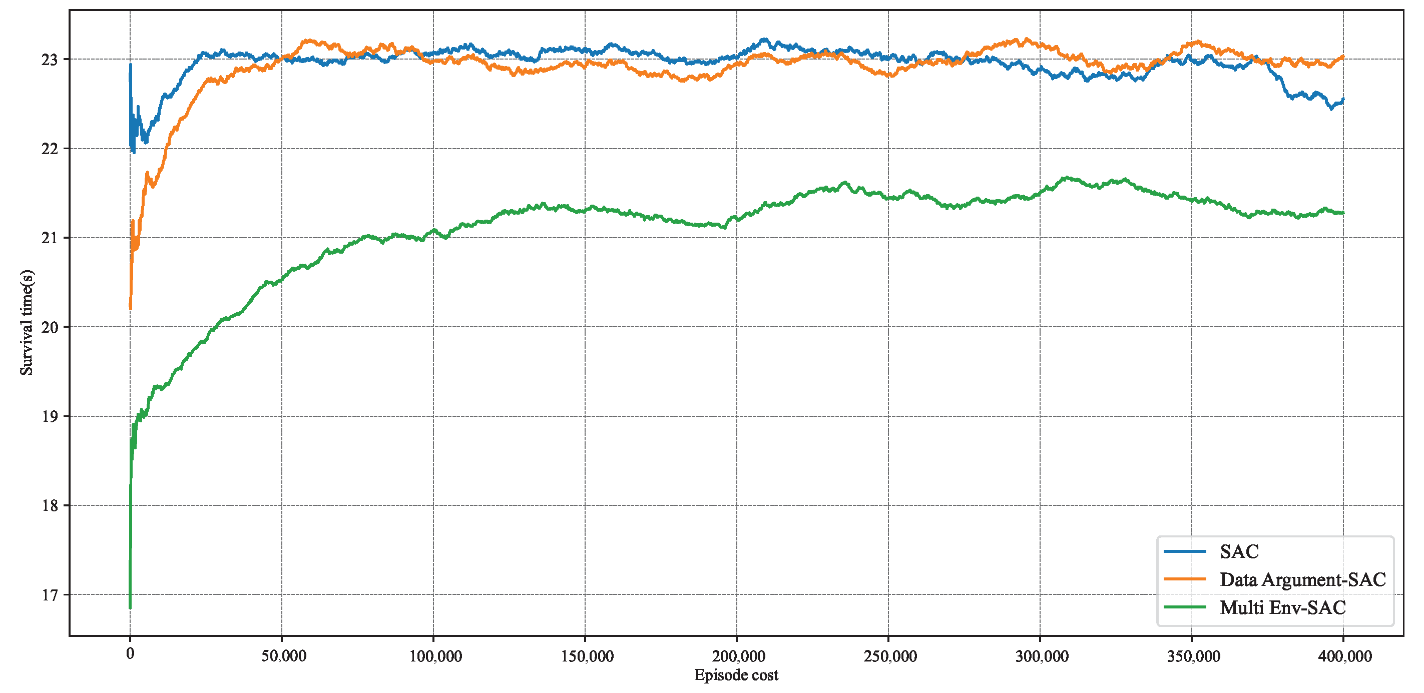
Figure 16 shows the training results of the three methods. It can be observed that after approximately 100,000 steps of iteration, the unprocessed reinforcement learning algorithm and Data Argument–SAC both achieved a high level of evasion capability, while Multi Env–SAC still exhibits a low level of evasion capability after 400,000 steps of training. The training results indicate that considering multiple different pursuers during the training phase greatly affects the algorithm’s convergence speed. This is because considering different pursuers makes the pursuit–evasion game problem more complex, and the additional dimensions in the state space mean that the reinforcement learning algorithm needs to interact with the environment on a larger scale to be trained, which implies that the required training time will increase to an unacceptable level. In contrast, Data Argument–SAC only processes the state signals during the training process and does not significantly affect training efficiency.

Figure 16.
Comparison of training results of three methods.
To further demonstrate the advantages of the MRPA algorithm in dealing with different pursuers, we conducted 3000 independent evasion experiments under scenarios where the pursuer’s proportional navigation constant was 4, 5, and 6, respectively. In each experiment, the MRPA algorithm and the evasion strategy trained by Data Argument–SAC were used to evade under the same initial conditions, and their survival times were recorded, as shown in Figure 17.

Figure 17.
Statistics of survival time of MRPA and Data Argument–SAC.
The experimental results show that using MRPA for policy adaptation allows for more survival time when dealing with different pursuers compared to the evasion strategy trained by Data Argument–SAC, demonstrating better generalization performance by the MRPA algorithm. The Data Argument–SAC method aims to enhance the robustness of reinforcement learning algorithms to potential noise interference in the environment through data augmentation. These noises are typically zero-mean noises, whereas changes in the pursuer’s pursuit strategy imply changes in the environment’s state transitions, which cannot be simply modeled as noise interference. Therefore, data augmentation techniques do not exhibit sufficient generalization performance in the scenarios discussed in this paper.
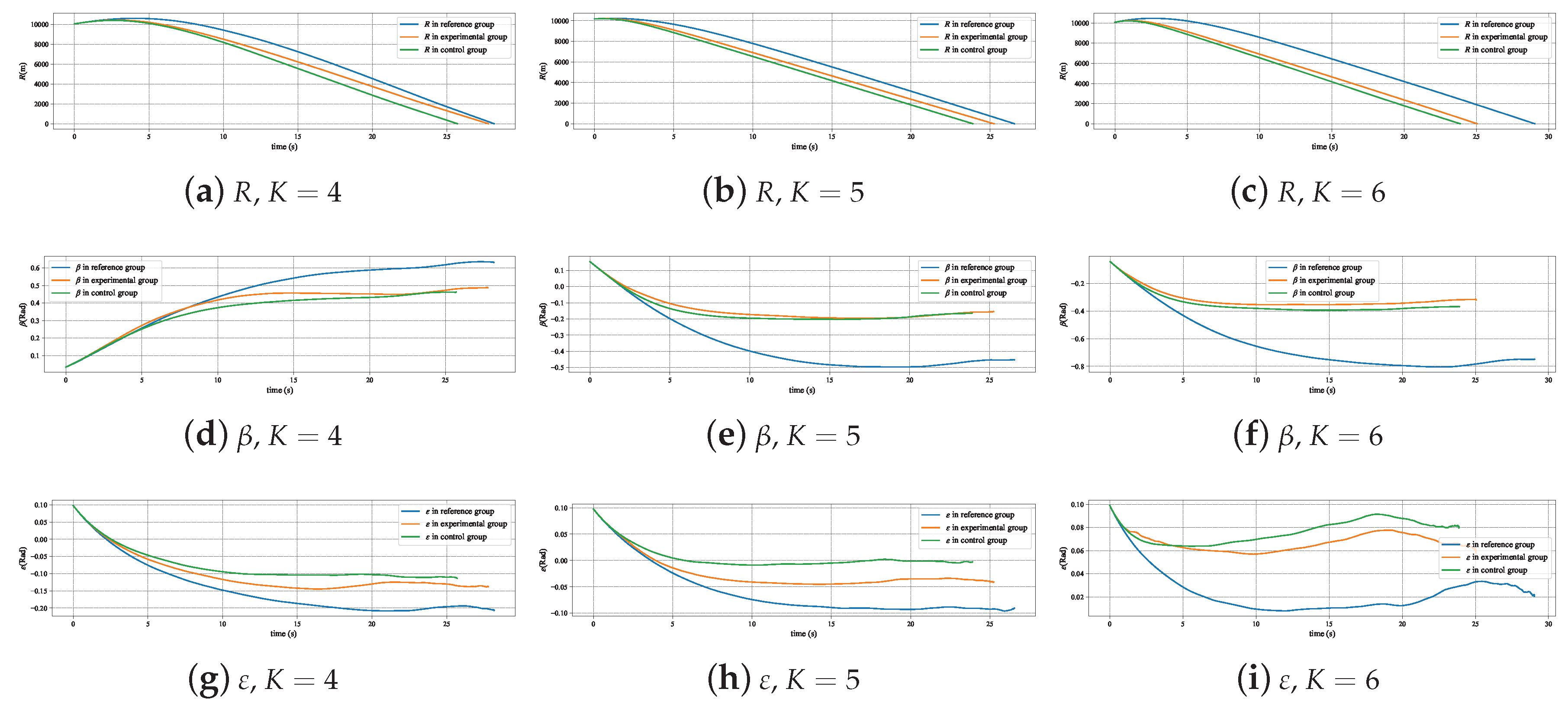
We conducted ablation experiments to validate the effectiveness of the MRPA algorithm. In the original environment, the reinforcement learning algorithm was trained to evade a pursuer with a proportional navigation constant , resulting in a reference policy. We conducted three tests, in which the proportional navigation constants of the pursuers in the test environment were 4, 5, and 6, respectively. Each test included an experimental group, a control group, and a reference group. All three groups loaded the reference policy. The experimental group evaded the test pursuer, loaded the policy trained in the original environment, and used the MRPA algorithm; the control group used the same pursuer and initial situation as the experimental group but did not use the MRPA algorithm; the reference group also used the same initial situation as the experimental group, evaded the pursuer used in the original environment, and did not use the MRPA algorithm. Each test was conducted with 3000 simulations through random initial situations, and the survival time of the experimental group, control group, and reference group in each simulation was recorded.
Figure 18 displays the typical trajectories of the evader and pursuer in three experiments, and it can be seen intuitively that the trajectory of the experimental group is significantly different from that of the reference group, even with a greater deviation than the control group. This is because the purpose of the MRPA algorithm to correct the UAV’s decision making commands is to make the changes in the relative position relationship between the experimental group’s evader and pursuer as close as possible to that of the reference group, which is determined by the state space of the Markov decision problem in the pursuit–evasion issue. The changes in relative distance, line-of-sight yaw angle, and line-of-sight pitch angle of the three typical cases shown in Figure 19 also illustrate that the deviations of several key states of the experimental group from the reference group are significantly smaller than those of the control group.

Figure 18.
Trajectories of evader and pursuer in three experiments.
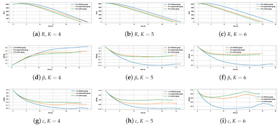
Figure 19.
Change in relative situation of typical cases in three experiments.
The experimental results shown in Figure 20 indicate that the experimental group using the MRPA algorithm with the reference policy can achieve better performance in evading pursuers different from the training environment. The reason for not reaching the same performance as the reference group lies in the fact that the dimension of the action vector in the pursuit–evasion game is less than that of the state vector. Consequently, the solution to Equation (72) is a least squares solution, which cannot ensure that the state transition is completely consistent with the reference model. Referring to the reward function’s setup, using a survival time of 24 s as the threshold to calculate the evasion success rate, Figure 21 demonstrates that the experimental group has improved by , , and over the control group in the three tests, respectively.

Figure 20.
Statistics of survival time of each group in ablation experiment.

Figure 21.
Evasion success rate statistics.
6. Conclusions
In response to the scenario of an unknown pursuer attacking an evader, an analytical method for estimating the pursuit UAV’s flight attitude and pursuit strategy was constructed through the analysis of the relative motion model of UAVs in pursuit–evasion games. Concurrently, a maneuvering evasion strategy was trained using a reinforcement learning algorithm, and a Model Reference Policy Adaptation (MRPA) algorithm was proposed to address different pursuers.
The results of numerical simulation indicate that the pursuit UAV’s flight attitude estimation and pursuit strategy identification can achieve a high accuracy, with response times less than 0.5 s. Moreover, the guidance law identification model can accurately track guidance law parameters that vary over time. The average error during the stable tracking phase is less than 2%. Comparative ablation experiments have shown that the MRPA algorithm can effectively enhance the performance of evasion strategies when dealing with unknown pursuers, with an average increase in evasion success rate of 8.4%.
Although it is assumed that the pursuer uses a proportional navigation guidance law, experimental results demonstrate that the guidance law parameter identification model is effective for dynamically changing parameters, and the MRPA algorithm, not being dependent on the specific guidance law construction, remains effective against pursuers employing a pursuit strategy.
7. Limitations and Future Work
Although comparative and ablation experiments demonstrate that the MRPA algorithm proposed in this paper can enable reinforcement learning-trained evasion strategies to effectively adapt to different pursuers, this method still has many limitations in practical use. The first limitation stems from the impact of observational noise. The MRPA algorithm needs to adjust decisions based on the results of pursuit strategy identification to adapt to different pursuers. The experimental results in Section 5.3 show that while the identification method proposed in this paper has some robustness to observational noise, noise still introduces higher errors into the identification results. Incorrect identification results can further reduce the robustness of the MRPA algorithm. Additionally, the modeling of the pursuit strategy in this paper has certain limitations. We use proportional navigation guidance to describe the pursuer’s strategy, but in reality, pursuers may employ a richer set of strategies, possibly including intelligent pursuit strategies trained by reinforcement learning algorithms. Although the method proposed in this paper can identify dynamically changing guidance law parameters, it cannot prove that it can represent all pursuit strategies. When we cannot correctly identify the pursuit strategy, the performance of the MRPA algorithm will inevitably decline.
In future work, we will conduct a more detailed modeling of the UAV pursuit–evasion game, such as considering more comprehensive aerodynamic constraints and potential time delays in control quantities, which will benefit the application of our method in the real world. Furthermore, we will use more advanced deep learning methods for pursuit strategy identification. By conducting large-scale simulations of different types and parameters of pursuit strategies to establish a dataset, we will train a deep learning model to directly identify the state transition matrix in Equation (57). This approach does not rely on specific kinematic models (e.g., Equations (14)–(16)) and may have better identification effects on different types of pursuit strategies. We hope these improvements will enable the MRPA algorithm to achieve better results in real-world environments.
Author Contributions
Conceptualization, Z.S., S.Z. and C.T.; Methodology, Z.S., Z.X. and W.F.; Software, Z.S., Z.X., C.T. and R.Q.; Validation, Z.X.; Formal analysis, Z.S. and S.Z.; Writing—original draft, Z.S.; Writing—review and editing, S.Z., Z.Z. and Y.X.; Supervision, Y.X.; Funding acquisition, L.C., Z.Z. and Y.X. All authors have read and agreed to the published version of the manuscript.
Funding
This research was funded by the Young Scientists Fund of the National Natural Science Foundation of China grant no. 52302506.
Data Availability Statement
The raw data supporting the conclusions of this article will be made available by the authors upon request.
DURC Statement
Current research is limited to the pursuit–evasion game of UAVs and application of reinforcement learning, which is beneficial in making the strategies trained by the reinforcement learning algorithm adapt to different environments (especially in the pursuit–evasion game scenario) and does not pose a threat to public health or national security. Authors acknowledge the dual-use potential of the research involving pursuit strategy identification and confirm that all necessary precautions have been taken to prevent potential misuse. As an ethical responsibility, authors strictly adhere to relevant national and international laws about DURC. Authors advocate for responsible deployment, ethical considerations, regulatory compliance, and transparent reporting to mitigate misuse risks and foster beneficial outcomes.
Conflicts of Interest
The authors declare no conflicts of interest.
References
- Qi, D.; Li, L.; Xu, H.; Tian, Y.; Zhao, H. Modeling and solving of the missile pursuit-evasion game problem. In Proceedings of the 2021 40th Chinese Control Conference (CCC), Shanghai, China, 26–28 July 2021; IEEE: Piscataway, NJ, USA, 2021; pp. 1526–1531. [Google Scholar]
- Perelman, A.; Shima, T.; Rusnak, I. Cooperative differential games strategies for active aircraft protection from a homing missile. J. Guid. Control. Dyn. 2011, 34, 761–773. [Google Scholar] [CrossRef]
- Rubinsky, S.; Gutman, S. Three-player pursuit and evasion conflict. J. Guid. Control. Dyn. 2014, 37, 98–110. [Google Scholar] [CrossRef]
- Karelahti, J.; Virtanen, K. Adaptive controller for the avoidance of an unknownly guided air combat missile. In Proceedings of the 2007 46th IEEE Conference on Decision and Control, New Orleans, LA, USA, 12–14 December 2007; IEEE: Piscataway, NJ, USA, 2007; pp. 1306–1313. [Google Scholar]
- Nakagawa, S.; Yamasaki, T.; Takano, H.; Yamaguchi, I. Timing determination algorithm for aircraft evasive maneuver against unknown missile acceleration. In Proceedings of the AIAA Scitech 2019 Forum, San Diego, CA, USA, 7–11 January 2019; p. 2344. [Google Scholar]
- Fonod, R.; Shima, T. Multiple model adaptive evasion against a homing missile. J. Guid. Control. Dyn. 2016, 39, 1578–1592. [Google Scholar] [CrossRef]
- Tian, Z.; Danino, M.; Bar-Shalom, Y.; Milgrom, B. Estimation-based missile threat detection and evasion maneuver for a low-altitude aircraft. In Proceedings of the Signal Processing, Sensor/Information Fusion, and Target Recognition XXXII, Orlando, FL, USA, 30 April–5 May 2023; SPIE: St. Bellingham, WA, USA, 2023; Volume 12547, pp. 27–35. [Google Scholar]
- Zhang, H.; Huang, C.; Zhang, Z.; Wang, X.; Han, B.; Wei, Z.; Li, Y.; Wang, L.; Zhu, W. The trajectory generation of UCAV evading missiles based on neural networks. In Journal of Physics: Conference Series; IOP Publishing: Bristol, UK, 2020; Volume 1486, p. 022025. [Google Scholar]
- Lillicrap, T.P.; Hunt, J.J.; Pritzel, A.; Heess, N.; Erez, T.; Tassa, Y.; Silver, D.; Wierstra, D. Continuous control with deep reinforcement learning. arXiv 2015, arXiv:1509.02971. [Google Scholar]
- Schulman, J.; Wolski, F.; Dhariwal, P.; Radford, A.; Klimov, O. Proximal policy optimization algorithms. arXiv 2017, arXiv:1707.06347. [Google Scholar]
- Haarnoja, T.; Zhou, A.; Abbeel, P.; Levine, S. Soft actor-critic: Off-policy maximum entropy deep reinforcement learning with a stochastic actor. In Proceedings of the International Conference on Machine Learning, PMLR, Stockholm, Sweden, 10–15 July 2018; pp. 1861–1870. [Google Scholar]
- Yu, C.; Velu, A.; Vinitsky, E.; Gao, J.; Wang, Y.; Bayen, A.; Wu, Y. The surprising effectiveness of ppo in cooperative multi-agent games. Adv. Neural Inf. Process. Syst. 2022, 35, 24611–24624. [Google Scholar]
- Bellemare, M.G.; Dabney, W.; Munos, R. A distributional perspective on reinforcement learning. In Proceedings of the International Conference on Machine Learning, PMLR, Sydney, Australia, 6–11 August 2017; pp. 449–458. [Google Scholar]
- Brunke, L.; Greeff, M.; Hall, A.W.; Yuan, Z.; Zhou, S.; Panerati, J.; Schoellig, A.P. Safe learning in robotics: From learning-based control to safe reinforcement learning. Annu. Rev. Control. Robot. Auton. Syst. 2022, 5, 411–444. [Google Scholar] [CrossRef]
- Kober, J.; Bagnell, J.A.; Peters, J. Reinforcement learning in robotics: A survey. Int. J. Robot. Res. 2013, 32, 1238–1274. [Google Scholar] [CrossRef]
- Tong, G.; Jiang, N.; Biyue, L.; Xi, Z.; Ya, W.; Wenbo, D. UAV navigation in high dynamic environments: A deep reinforcement learning approach. Chin. J. Aeronaut. 2021, 34, 479–489. [Google Scholar]
- Fei, W.; Xiaoping, Z.; Zhou, Z.; Yang, T. Deep-reinforcement-learning-based UAV autonomous navigation and collision avoidance in unknown environments. Chin. J. Aeronaut. 2024, 37, 237–257. [Google Scholar]
- Lupu, A.; Cui, B.; Hu, H.; Foerster, J. Trajectory diversity for zero-shot coordination. In Proceedings of the International Conference on Machine Learning, PMLR, Virtual, 18–24 July 2021; pp. 7204–7213. [Google Scholar]
- Jiang, Y.; Liu, Q.; Ma, X.; Li, C.; Yang, Y.; Yang, J.; Liang, B.; Zhao, Q. Learning Diverse Risk Preferences in Population-Based Self-Play. In Proceedings of the AAAI Conference on Artificial Intelligence, Vancouver, BC, Canada, 20–27 February 2024; Volume 38, pp. 12910–12918. [Google Scholar]
- Bansal, T.; Pachocki, J.; Sidor, S.; Sutskever, I.; Mordatch, I. Emergent complexity via multi-agent competition. arXiv 2017, arXiv:1710.03748. [Google Scholar]
- Balduzzi, D.; Garnelo, M.; Bachrach, Y.; Czarnecki, W.; Perolat, J.; Jaderberg, M.; Graepel, T. Open-ended learning in symmetric zero-sum games. In Proceedings of the International Conference on Machine Learning, PMLR, Long Beach, CA, USA, 9–15 June 2019; pp. 434–443. [Google Scholar]
- Özbek, M.M.; Koyuncu, E. Missile Evasion Maneuver Generation with Model-free Deep Reinforcement Learning. In Proceedings of the 2023 10th International Conference on Recent Advances in Air and Space Technologies (RAST), Istanbul, Turkey, 7–9 June 2023; pp. 1–6. [Google Scholar] [CrossRef]
- Huang, C.; Wang, C.; Chai, S.; Tong, Q.; Li, Y. Research on Evasion Policy of UCAV Against Infrared Air-to-Air Missile Based on Soft Actor Critic Algorithm. In Proceedings of the 14th International Conference on Computer Modeling and Simulation, Chongqing, China, 24–26 June 2022; pp. 153–159. [Google Scholar]
- Yan, M.; Yang, R.; Zhang, Y.; Yue, L.; Hu, D. A hierarchical reinforcement learning method for missile evasion and guidance. Sci. Rep. 2022, 12, 18888. [Google Scholar] [CrossRef] [PubMed]
- Hou, Y.; Liang, X.; Lv, M.; Yang, Q.; Li, Y. Subtask-masked curriculum learning for reinforcement learning with application to UAV maneuver decision-making. Eng. Appl. Artif. Intell. 2023, 125, 106703. [Google Scholar] [CrossRef]
- Lam, V. Time-to-go estimate for missile guidance. In Proceedings of the AIAA Guidance, Navigation, and Control Conference and Exhibit, San Francisco, CA, USA, 15–18 August 2005; p. 6459. [Google Scholar]
- Ralph, J.F.; Smith, M.I.; Heather, J.P. Identification of missile guidance laws for missile warning systems applications. In Proceedings of the Signal and Data Processing of Small Targets, Kissimmee, FL, USA, 18–20 April 2006; SPIE: St. Bellingham, WA, USA, 2006; Volume 6236, pp. 87–98. [Google Scholar]
- Yun, J.; Ryoo, C.K. Missile guidance law estimation using modified interactive multiple model filter. J. Guid. Control. Dyn. 2014, 37, 484–496. [Google Scholar] [CrossRef]
- Wang, Y.; Wang, J.; Fan, S.; Li, L. Online time-varying navigation ratio identification and state estimation of cooperative attack. Aerosp. Sci. Technol. 2023, 136, 108261. [Google Scholar] [CrossRef]
- Wang, Y.; Wang, J.; Fan, S. Parameter Identification of a PN-Guided Incoming Missile Using an Improved Multiple-Model Mechanism. IEEE Trans. Aerosp. Electron. Syst. 2023, 59, 5888–5899. [Google Scholar] [CrossRef]
- Yinhan, W.; Shipeng, F.; Jiang, W.; Guang, W. Quick identification of guidance law for an incoming missile using multiple-model mechanism. Chin. J. Aeronaut. 2022, 35, 282–292. [Google Scholar]
- Oh, J.; Singh, S.; Lee, H.; Kohli, P. Zero-shot task generalization with multi-task deep reinforcement learning. In Proceedings of the International Conference on Machine Learning, PMLR, Sydney, Australia, 6–11 August 2017; pp. 2661–2670. [Google Scholar]
- Sohn, S.; Oh, J.; Lee, H. Hierarchical reinforcement learning for zero-shot generalization with subtask dependencies. Adv. Neural Inf. Process. Syst. 2018, 31. [Google Scholar]
- Raileanu, R.; Goldstein, M.; Yarats, D.; Kostrikov, I.; Fergus, R. Automatic data augmentation for generalization in deep reinforcement learning. arXiv 2020, arXiv:2006.12862. [Google Scholar]
- Hansen, N.; Wang, X. Generalization in reinforcement learning by soft data augmentation. In Proceedings of the 2021 IEEE International Conference on Robotics and Automation (ICRA), Xi’an, China, 30 May–5 June 2021; IEEE: Piscataway, NJ, USA, 2021; pp. 13611–13617. [Google Scholar]
- Ball, P.J.; Lu, C.; Parker-Holder, J.; Roberts, S. Augmented world models facilitate zero-shot dynamics generalization from a single offline environment. In Proceedings of the International Conference on Machine Learning, PMLR, Virtual, 18–24 July 2021; pp. 619–629. [Google Scholar]
- Niv, Y.; Joel, D.; Meilijson, I.; Ruppin, E. Evolution of reinforcement learning in uncertain environments: A simple explanation for complex foraging behaviors. Int. Soc. Adapt. Behav. 2002, 10, 5–24. [Google Scholar]
- Peng, X.B.; Andrychowicz, M.; Zaremba, W.; Abbeel, P. Sim-to-real transfer of robotic control with dynamics randomization. In Proceedings of the 2018 IEEE International Conference on Robotics and Automation (ICRA), Brisbane, Australia, 21–26 May 2018; IEEE: Piscataway, NJ, USA, 2018; pp. 3803–3810. [Google Scholar]
- Ghosh, D.; Rahme, J.; Kumar, A.; Zhang, A.; Adams, R.P.; Levine, S. Why generalization in rl is difficult: Epistemic pomdps and implicit partial observability. Adv. Neural Inf. Process. Syst. 2021, 34, 25502–25515. [Google Scholar]
- Sutton, R.S.; McAllester, D.; Singh, S.; Mansour, Y. Policy gradient methods for reinforcement learning with function approximation. Adv. Neural Inf. Process. Syst. 1999, 12. [Google Scholar]
- Nguyen, N.T.; Nguyen, N.T. Model-Reference Adaptive Control; Springer: Berlin/Heidelberg, Germany, 2018. [Google Scholar]
- Parks, P. Liapunov redesign of model reference adaptive control systems. IEEE Trans. Autom. Control 1966, 11, 362–367. [Google Scholar] [CrossRef]
- Guerrero-Sánchez, M.E.; Hernández-González, O.; Valencia-Palomo, G.; López-Estrada, F.R.; Rodríguez-Mata, A.E.; Garrido, J. Filtered observer-based ida-pbc control for trajectory tracking of a quadrotor. IEEE Access 2021, 9, 114821–114835. [Google Scholar] [CrossRef]
Disclaimer/Publisher’s Note: The statements, opinions and data contained in all publications are solely those of the individual author(s) and contributor(s) and not of MDPI and/or the editor(s). MDPI and/or the editor(s) disclaim responsibility for any injury to people or property resulting from any ideas, methods, instructions or products referred to in the content. |
© 2024 by the authors. Licensee MDPI, Basel, Switzerland. This article is an open access article distributed under the terms and conditions of the Creative Commons Attribution (CC BY) license (https://creativecommons.org/licenses/by/4.0/).

