Bifurcation Analysis and Sticking Phenomenon for Unmanned Rotor-Nacelle Systems with the Presence of Multi-Segmented Structural Nonlinearity

Abstract

Whirl flutter is a phenomenon caused by an aeroelastic instability, causing oscillations to propagate in manned or unmanned rotor-nacelle type aircraft. Under the conditions where multi-segmented freeplay are present, complex behaviors can dominate these oscillations and can lead to disastrous consequences. This study investigates a rotor-nacelle system with multi-segmented stiffnesses with a freeplay gap to encompass the real-world influences of aircraft. The mathematical aerodynamics model considers a quasi-steady application of strip theory along each blade to outline the external forces being applied. A free-body diagram is then used to incorporate the structural stiffness and damping terms with multi-segmented freeplay considered in the structural stiffness matrix. Multiple structural responses of the defined system are investigated and characterized to determine the influence of varying symmetric and asymmetric multi-segmented stiffnesses with varying gap parameters, including a route to impact investigation. The findings are characterized using phase portraits, Poincaré maps, time histories, and basins of attraction. It is found that under these conditions, the structural influences can lead to aperiodic oscillations with the existence of grazing bifurcations. Furthermore, these results unveil that under certain conditions and high freestream velocities, the sticking phenomenon becomes apparent which is strongly dependent on the strength of the multi-segmented representation, its gap sizes, and its symmetry. Lastly, a route to impact study shows the strong coupled influence between pitch and yaw when asymmetric conditions are applied and the possible presence of grazing-sliding bifurcations. The numerical simulations performed in this study can form a basis for drone designers to create reliable rotor-nacelle systems resistant to whirl flutter caused by freeplay effects.

1. Introduction

The modernization of aircraft has advanced flight time, speed, and maneuverability over the past century [1,2,3]. However, the aeroelastic phenomenon still limits aircraft operation and must be considered when designing and building these systems. These challenges are particularly cumbersome when referring to manned or unmanned rotor-nacelle type aircraft, as they are a simpler, cheaper, and sometimes a better option than their jet propulsion counterpart, considering specific mission characteristics. Therefore, the challenges of the rotor-nacelle-driven design must be studied, characterized, and considered when designing. One particular challenge in historic failures is the structural effects of an aeroelastic instability known as whirl flutter. The physical phenomenon of whirl flutter creates structural oscillations in an aircraft system, and depending on the growth rate and severity of these oscillations, whirl flutter can cause unstable flight performance. In the most severe cases, catastrophic structural failure can result [4].

Taylor first discovered whirl flutter from the Massachusetts Institute of Technology and Browne from Wright Aeronautical Corporation in 1938 [5]. Preliminary research on the topic did not receive much attention and was dismissed as not being a legitimate concern until 1960. That year, NASA lost two turboprop aircraft due to the aeroelastic instability of the rotor-nacelle [6,7]. The onset of whirl flutter has been shown to damage surrounding structures of the rotor-nacelle, especially the mount location and wing depending on the mounting position. The onset of whirl flutter results from a coupling between the structure wing/mounting material, the aerodynamic forces and moments on the rotor, and the gyroscopic effect of the rotor [8,9,10]. Depending on the aircraft type and the rotor-nacelle’s location, the system may respond differently when aeroelastic instability occurs. For instance, in Vertical-Take-Off-and-Landing (VTOL) systems, additional coupling terms are present, which are not seen in helicopters [11].

The events with the Lockheed L-188c Electra aircraft were an iconic example of failure caused by whirl flutter. This aircraft had its first flight in 1957 and was the first large-scale turboprop airliner built in the United States [12]. On 17 March 1960, a Lockheed Electra model L-188c, owned and operated by Northwest Airlines, Inc, crashed after the failure of its right-wing [13]. All 63 passengers and crew perished in the accident. Following the failure of this aircraft, a panel of experts was assembled to determine the cause of the incident. Their conclusions, stated in the accident report, were: “The Board determines that the probable cause of this accident was the separation of the right-wing in flight due to flutter induced by oscillations of the outboard nacelles” [13]. A second Lockheed Electra model L-188c crashed only months later, killing all passengers aboard.

Whirl flutter has caused concern in propeller-driven, tilt-rotor, and helicopter aircraft, brought on by the two Lockheed Electra planes that crashed. Whirl flutter, the aeroelastic phenomenon of oscillatory behavior caused by the rotation of the propeller, exasperated by freestream airflow, can be catastrophic to aircraft. These repetitive oscillations fatigue the material and connection joints that mount the rotor-nacelle assembly. Depending on an aircraft’s size, weight, and mission parameters, there can be various methods of mounting the rotor-nacelle to the wing. For example, in small-scale, lightweight designs, such as micro unmanned aerial vehicles (i.e., drones), the engine can be glued or screwed to the wing’s surface [14,15,16]. The most common method of mounting an engine to a wing utilizes a pylon to attach the two components [17]. However, both attachments rely on attaching the surfaces in mounting the engine to the pylon and the pylon to the wing. The risk of loosening attachments due to vibration or fatigue becomes a real possibility if regular maintenance is neglected. As these attachments loosen when the system’s vibration starts, freeplay is introduced, and this effect can be disastrous to the structural integrity of the aircraft. Freeplay is one of the most common paths to failure with contact materials which undergo repetitive oscillatory motion known as “joint backlash” [18].

A two-degree-of-freedom rotor nacelle assembly can provide valuable insight and information on the physical nature of the aeroelastic phenomenon of whirl flutter. Most of the research on this aeroelastic phenomenon focuses on the linear structural stiffness responses and is limited to the possible existence of nonlinearities and/or freeplay in the pitch and/or yaw degrees of freedom [19,20,21,22]. In the research performed by Mair et al. [19], the authors looked into the impact of nonlinear pylon stiffness on whirl flutter stability. This study demonstrated the coexistence of stable and unstable limit cycles in the nonlinear system, while focusing on the importance of the nonlinear whirl flutter model and analysis method. Further investigation was examined by Mair et al. [20] where they studied the inclusion of freeplay in tiltrotor aircraft design. The findings of the study outlined the effects of freeplay on the model complexity and deadband edge sharpness. Quintana et al. [21] investigated the whirl flutter phenomenon on an unmanned rotor-nacelle system under linear and nonlinear stiffnesses, to characterize the behavioral responses and identify key influential features. Based on this research, it was discovered that the whirl flutter effect on the system is strongly influenced by two key factors: the angular velocity of the rotor and the number of blades. Moreover, in a subsequent study by Quintana et al. [22], the inclusion of freeplay was studied for various symmetrically and asymmetrically applied nonlinear cubic stiffness. The study identified and characterized key behavioral responses based on freeplay limits, key features, and grazing contacts, as well as the coupled effects of the pitch and yaw.

Due to the possible presence of increased stiffness at higher oscillations with the existence of the freeplay nonlinearity, multi-segmented representation for the structural moment or force depending on the region of oscillation was introduced in previous studies [23,24]. Indeed, multi-segmented modeling has been used to describe various types of structural stiffnesses in different dynamical systems, such as flutter-based aeroelastic systems [23] and energy harvesting systems from flow-induced vibrations [24]. Vasconcellos et al. [23] focused on the effects of a multi-segmented nonlinear two-degree of freedom aeroelastic control surface. In the study, it was shown that the system undergoes several transitions in response to increased wind speeds and encounters grazing contact, which leads to grazing bifurcation. A grazing contact occurs when the amplitude of the system response just comes into contact with a contact surface, such as when a gap between moving parts is fully closed. A grazing bifurcation occurs when the variation in some system parameters brings the system to a grazing contact which causes a bifurcation of any sort. In the study conducted by Bouma et al. [24], the authors analyzed a two-degree of freedom piezoaeroelastic energy harvesting system that incorporates multi-segmented freeplay. In the investigation, the presence of nonlinearities allowed for energy harvesting at lower wind speed than its linear counterpart, with the strength of the nonlinearity affecting the systems dynamics at low pitch angles.

Multi-segment stiffness can be a real concern when dealing with rotor-nacelle systems, as joints or attachments frequently present regions of freeplay, and a second discontinuous transition to higher stiffness due to stoppers or other mechanical properties of the structure at higher amplitude oscillations. To explore the possible effects of multi-segmented stiffnesses on the dynamical responses of rotor-nacelle systems, this study focuses on applying multi-segmented freeplay parameters symmetrically and asymmetrically to the pitch and yaw degrees of freedom. The multi-segmentation is considered based on the structure deflections caused by whirl flutter, which lead to a nonsmoothed stiffness function comprising different stiffness regions including freeplay. The overall goal of this work is to evaluate the onset of whirl flutter under these conditions of piecewise freeplay. This would allow for the future inclusion of early warning systems or active control damping systems to prevent catastrophic failures. Section 2 begins with an outline of the mathematical model, the considered parameters and conditions, and the solution method used. Next, Section 3, investigates the bifurcation response with various symmetric and asymmetric gap sizes, from which the trends and behaviors are identified, analyzed, and characterized. Section 4 of this study characterizes the bifurcation behaviors resulting from the route to impact of several symmetric and configurations. Finally, Section 4 summarizes main conclusions and results outline in this research study.

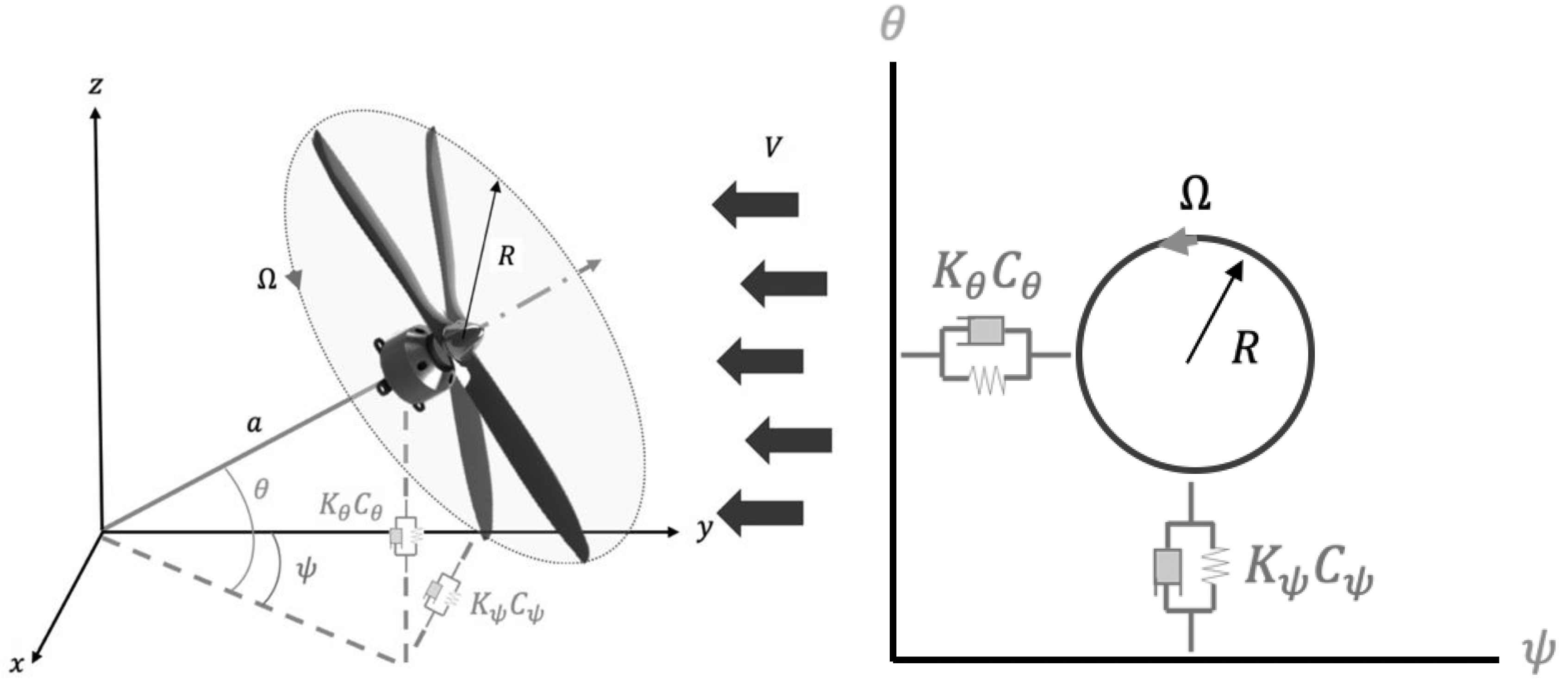
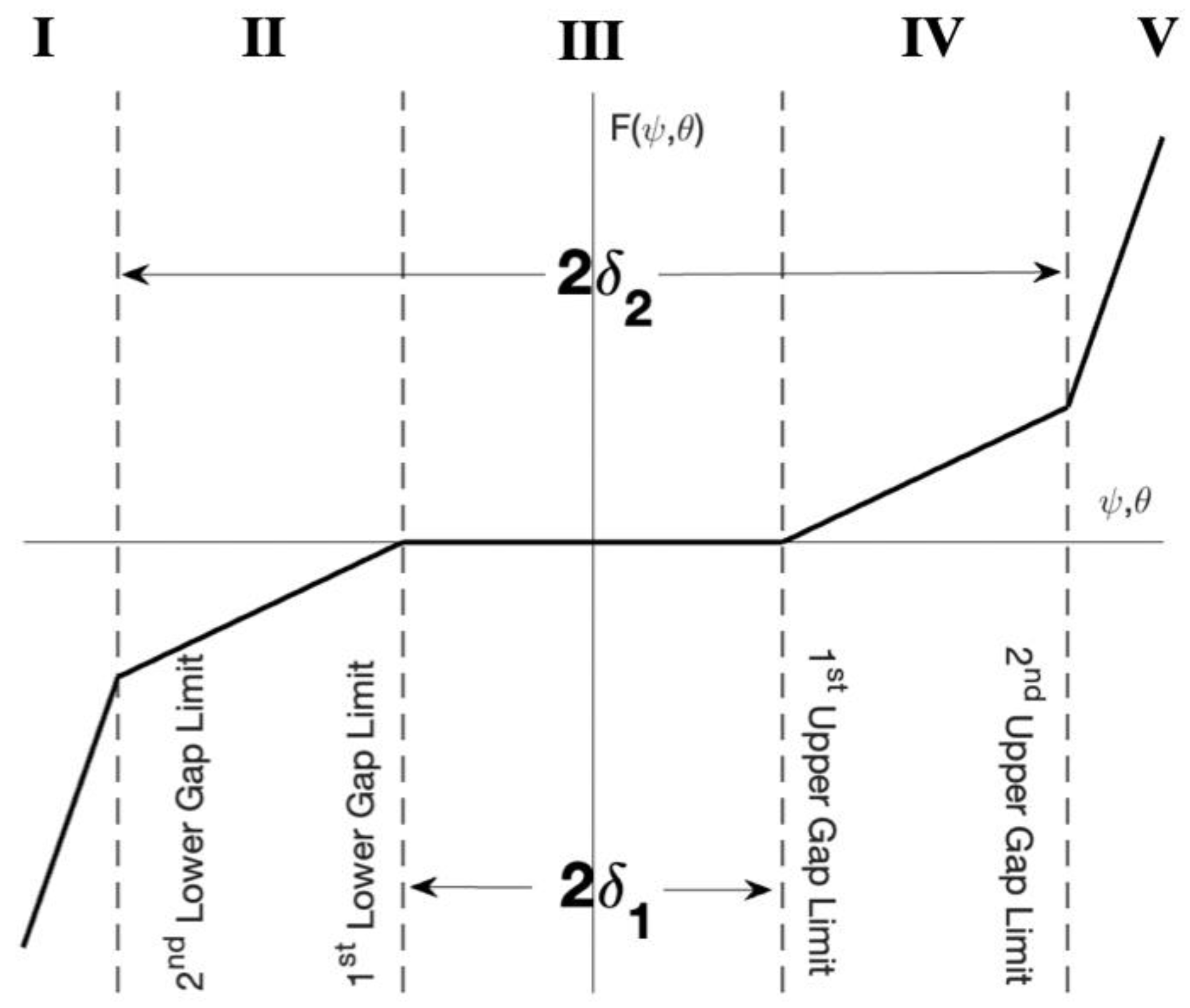
2. Aeroelastic Modeling of Multi-Segmented Freeplay System

In order to study the whirl flutter effects, a free body diagram must be considered in which to create the equations of motion, as well as the external moments in the mathematical model. Therefore, the simplest solution is to consider an operational aircraft with the given conditions: it must be driven by a rotor-nacelle, and there must be extensive information regarding its geometric and dynamic properties. A mathematical reduced-order model was developed by Reed [7] and Bielawa [25] and was applied in this study to incorporate the real-world conditions of multi-segmented freeplay seen in oscillating structural dynamic problems.

The free body diagram is depicted in Figure 1 to model the aerodynamic system mathematically. Off the initial position, considered to be on the y-axis, the rotor-nacelle is free to move in the pitch and yaw directions, $\theta$ and $\psi$, respectively. The motion of the rotor-nacelle is controlled by springs and dampers, $K_{\theta }$ and $K_{\psi },$ representing the spring coefficients, and $C_{\theta }$ and $C_{\psi },$ representing the damping coefficients. The direction the rotor is spinning by a positive $\Omega$, with the rotor radius being $R$ off the lever arm $a$. The freeplay gap is considered along the pitch and yaw directions, the z-axis and x-axis, respectively. Finally, the arrows show the freestream velocity, $V$, with the positive flow towards the rotor-nacelle. This free body diagram is then used to derive the governing equations of motion for the coupled second-order ordinary differential equation system.

The governing equations of motion, given in Equation (1), outline the response of the system in pitch and yaw [7,19,20,25]:

$$\left[\begin{array}{cc}{I}_n& 0\\ 0& I_n\end{array}\right]\left\{\begin{array}{c}\ddot{\theta }\\ \ddot{\psi }\end{array}\right\}+\left[\begin{array}{cc}{C}_{\theta }& -I_x\Omega \\ I_x\Omega & C_{\psi }\end{array}\right]\left\{\begin{array}{c}\dot{\theta }\\ \dot{\psi }\end{array}\right\}+\left[\begin{array}{cc}\frac{K_{\theta }F\left(\theta \right)}{\theta }& 0\\ 0& \frac{K_{\psi }F\left(\psi \right)}{\psi }\end{array}\right]\left\{\begin{array}{c}\theta \\ \psi \end{array}\right\}=\left[\begin{array}{c}{M}_{\theta }\\ M_{\psi }\end{array}\right]$$

(1)

The aerodynamic forces on airfoils were thoroughly investigated by Bielawa [25]. He employed the quasi-steady strip theory to provide a detailed understanding of the aerodynamics of airflow over the propeller blades of a rotor-nacelle. This theory considered the interaction between airflow and airfoil surfaces, including the effects of in-plane blade elastic deformations. By studying the motion of the blades using a generalized coordinate, he observed a distortion of the membrane within the plane of rotation. He was then able to describe lift distribution at the airfoil section in relation to dynamic pressure and angle of attack. Bielawa [25] used this lift distribution to determine cumulative perturbational in-plane forces, as well as pitching and rolling moments at the hub, accounting for all blades. It should be mentioned that the analysis assumed quasi-steady conditions which assumes small angles of attack and small reduced frequency [7,19,20,26]. This data are advantageous because it is difficult to perform this kind of study on a commercial tilt-rotor system. Reed [7] performed this type of experiment on a scaled-down aircraft in a wind tunnel, and Mair et al. [19,20] later performed two studies using the same system as a reference. A similar wind tunnel rotor-nacelle system is considered in this study.

Using the lift calculated along each blade for a specified number of propellers, and breaking them into their respective directional component in the pitch and yaw axis, the following moments in Equations (2) and (3) are developed [7,19,20,25,26]:

$$M_{\theta }=\frac{N_B}{2}\left(\frac{1}{2}\rho c_{l,{\alpha }_3}{R}^4{\Omega }^2\right)R\left[-\left(A_3+a^2{A}_1\right)\frac{\dot{\theta }}{\Omega }-A_2^{\prime }\psi +a{A}_1^{\prime }\theta \right]$$

(2)

$$M_{\psi }=\frac{N_B}{2}\left(\frac{1}{2}\rho c_{l,{\alpha }_3}{R}^4{\Omega }^2\right)R\left[-\left(A_3+a^2{A}_1\right)\frac{\dot{\psi }}{\Omega }+A_2^{\prime }\theta +a{A}_1^{\prime }\psi \right]$$

(3)

By reorganizing Equations (2) and (3) into Equation (1) and formatting it into the required form, it becomes possible to solve the ordinary differential equation with the Jacobian method. Based on the previous moment terms, the stiffness and damping matrices are then rewritten and decomposed into their aerodynamic and structural components as shown in Equations (4) and (5) as follows:

$$\left[C\right]=\left[\begin{array}{cc}{C}_{\theta }+\frac{c_{K,a}\left(A_3+a^2{A}_1\right)}{\Omega }& -I_x\Omega \\ I_x\Omega & C_{\psi }+\frac{c_{K,a}\left(A_3+a^2{A}_1\right)}{\Omega }\end{array}\right]$$

(4)

$$\left[K\right]=\left[\begin{array}{cc}\frac{K_{\theta }F\left(\theta \right)}{\theta }-c_{K,a}a\beta A_1& c_{K,a}{A}_2\\ -c_{K,a}{A}_2& \frac{K_{\psi }F\left(\psi \right)}{\psi }-c_{K,a}a\beta A_1\end{array}\right]$$

(5)

where $\beta$ denotes the velocity ratio of freestream velocity to velocity at the blade tip shown in Equation (6) as:

$$\beta =\frac{V}{R\Omega }=\frac{V}{V_{tip}}$$

(6)

and the consolidated terms used in Equations (7)–(10) are given by [19,20,22]:

$$c_{K,a}=\frac{N_B}{2}\left(\frac{1}{2}\rho c_{l,{\alpha }_3}{R}^4{\Omega }^2\right)R$$

(7)

$$A_1=\frac{c}{R}{\int }_0^1\frac{{\beta }^2}{\sqrt{{\beta }^2+{\gamma }^2}}d\gamma$$

(8)

$$A_2=\frac{c}{R}{\int }_0^1\frac{{\beta }^2{\gamma }^2}{\sqrt{{\beta }^2+{\gamma }^2}}d\gamma$$

(9)

$$A_3=\frac{c}{R}{\int }_0^1\frac{{\gamma }^4}{\sqrt{{\beta }^2+{\gamma }^2}}d\gamma$$

(10)

Utilizing the equations of motion shown in Equation (1) and considering the aerodynamic loads, a solution method can then be applied. By reformatting the equations of motion, the following Jacobian matrix is developed [19,20]:

$$J=\left[\begin{array}{cc}\left[0\right]& \left[I\right]\\ -{\left[\begin{array}{cc}{I}_n& 0\\ 0& I_n\end{array}\right]}^{-1}\left[K\right]& -{\left[\begin{array}{cc}{I}_n& 0\\ 0& I_n\end{array}\right]}^{-1}\left[C\right]\end{array}\right]$$

(11)

where, $\mathit{Z}={[\theta \psi \dot{\theta } \dot{\psi }]}^{\mathit{T}}$ is the state vector, and the state-space form is:

$$\dot{\mathit{Z}}=J\mathit{Z}$$

(12)

In order to complete the mathematical model, the geometric and dynamic parameters of the scaled wind tunnel rotor-nacelle unmanned system are listed in

Table 1. List of geometric and dynamic properties for the scaled wind tunnel rotor-nacelle system [7,19,20].

Description	Symbol	Value	Description	Symbol	Value
Rotor radius	R	0.152 m	Structural pitch damping	$C_{\theta }$	0.001 Nm s rad−1
Rotor angular velocity	$\Omega$	40 rad s−1	Structural pitch stiffness	$K_{\theta }$	0.4 Nm rad−1
Freestream velocity	V	6.7 m s−1	Structural yaw damping	$C_{\psi }$	0.001 Nm s rad−1
Air density	$\rho$	1.2 kg m−3	Structural yaw stiffness	$K_{\psi }$	0.4 Nm rad−1
Pivot length to rotor radius ratio	$a$	0.25	Number of blades	$N_B$	4
Rotor moment of inertia	$I_x$	0.000103 kg m2	Blade chord	c	0.026 m
Nacelle moment of inertia	$I_n$	0.000178 kg m2	Blade lift slope	$c_{l,{\alpha }_3}$	$2\pi$ rad−1

. These parameters include the rotor radius, rotor angular velocity, structural moments, linear stiffnesses, damping coefficients, and propeller specification. These parameters can then be included in the mathematical model, with one exception; the structural stiffness needs to be restructured to account for the multi-segmented freeplay condition as per the main contribution and focus of this work.

As previously discussed, aeroelastic systems can be subjected to a variety of structural stiffness regions including freeplay. Therefore, a multi-segmented stiffness is considered in this study because of the case when the oscillatory motion of rotor-nacelle impacts increased stiffness control surfaces, where the resulting impact can influence the system’s response. Moreover, the freeplay in the system must be considered because of nonlinear influences in the system, such as the loosening contact between the rotor-nacelle and platform on which the motor is mounted, caused by fatigue or improper maintenance. The multi-segmented stiffness model allows for a study into the system’s response under multiple stiffness regions which can be present, and it helps determine the characteristic behavior observed.

To effectively develop this stiffness model, a piecewise function is developed with the consideration of two gap conditions, ${\delta }_1$ and ${\delta }_2$, where the ${\delta }_1$ bounds the freeplay, ${\delta }_2$ bounds the first linear stiffness, and beyond the ${\delta }_2$ results in the second linear stiffness which are characterized by two hardening stiffness multipliers, n and m. The stiffnesses of the yaw and pitch springs are based on a combination of five stiffness regions with freeplay and stoppers that can be adjusted between flexible or hard impact. The representation of the stiffness with multi-segmented freeplay and stoppers in the pitch and yaw, F($\theta$) and F($\psi$), respectively, is given by Equations (13) and (14):

$$F\left(\theta \right)=\left\{\begin{array}{l}n\theta +{\delta }_{1\theta }+\left(n-1\right){\delta }_{2\theta } if \theta <-{\delta }_{2\theta } \\ \theta +{\delta }_{1\theta } if -{\delta }_{2\theta }<\theta <-{\delta }_{1\theta } \\ 0 if \left|\theta \right| \le {\delta }_{1\theta } \\ \theta -{\delta }_{1\theta } if {\delta }_{2\theta }>\theta > {\delta }_{1\theta } \\ n\theta -{\delta }_{1\theta }-\left(n-1\right){\delta }_{2\theta } if \theta > {\delta }_{2\theta } \end{array}\right.$$

(13)

$$F(\psi )=\left\{\begin{array}{l}m\psi +{\delta }_{1\psi }+\left(m-1\right){\delta }_{2\psi } if \psi <-{\delta }_{2\psi } \\ \psi +{\delta }_{1\psi } if -{\delta }_{2\psi }<\psi <-{\delta }_{1\psi } \\ 0 if \left|\psi \right| \le {\delta }_{1\psi } \\ \psi -{\delta }_{1\psi } if {\delta }_{2\psi }>\psi > {\delta }_{1\psi } \\ m\psi -{\delta }_{1\psi }-\left(m-1\right){\delta }_{2\psi } if \psi > {\delta }_{2\psi } \end{array}\right.$$

(14)

The two stiffness equations create five distinct stiffness response regions for multi-segmented stiffness, as shown in Figure 2: (I) when ${\delta }_{2\left\{\psi , \theta \right\}}$ is less than $\left\{\psi , \theta \right\}$, the stiffness is reliant upon a multiplier term n or m in the negative F($\psi , \theta$) area; (II) when $\left\{\psi , \theta \right\}$ is between the gap limit ${\delta }_{1\left\{\psi , \theta \right\}}$ and ${\delta }_{2\left\{\psi , \theta \right\}}$, the stiffness is defined by the table minus the ${\delta }_{1\left\{\psi , \theta \right\}}$ gap; (III) when $\left|\left\{\psi , \theta \right\}\right|$ is less than or equal to the ${\delta }_{1\left\{\psi , \theta \right\}}$ gap, the freeplay region will be zero; (IV) when $\left\{\psi , \theta \right\}$ is between the gap limit $-{\delta }_{1\left\{\psi , \theta \right\}}$ and $-{\delta }_{2\left\{\psi , \theta \right\}}$, the stiffness is defined by the table plus the ${\delta }_{1\left\{\psi , \theta \right\}}$ gap; and (V) when ${\delta }_{2\left\{\psi , \theta \right\}}$ is less than $\left\{\psi , \theta \right\}$, the stiffness is reliant upon a multiplier term n or m in the positive F($\psi , \theta$) area.

Lastly, the method used to solve the ordinary differential equation can then be iteratively solved using the MATLAB ODE45 built-in function [27]. The ODE45 operates as a sub-function, with inputs of time, initial conditions, and a simplified Jacobian matrix. Furthermore, before entering the ODE45 ordinary differential solver, an application of event location is considered at and around the freeplay boundaries ${\delta }_1$ and ${\delta }_2$. The event location function allows for an increase in accuracy at and around the gap limits due to the possibility of accumulating error from over- or under-estimating the contact around these regions. It should be noted that for the bifurcation diagrams, the maximum and minimum peaks of the resulting oscillations are plotted in order to characterize the response of the system. The numerical techniques employed in this study were used mainly for convenience, but alternative forms of analysis are possible, such as analytically determining the stability and bifurcations of the system or performing numerical continuation to trace out solution curves. Numerical results are characterized in several ways: using phase portraits, Poincaré maps, time histories, and basins of attraction. Phase portraits are plots of the system’s state space (plots of a coordinate vs. the time derivative of the coordinate, e.g., pitch angle vs. pitch angular velocity); a Poincaré map is the set of points residing on a plane that intersects the flow of the system response in state space; and a basin of attraction is the set of initial condition points that all lead to the same steady-state system response.

3. Bifurcation Analysis and Characterization of Rotor-Nacelle Systems with Multi-Segmented Freeplay

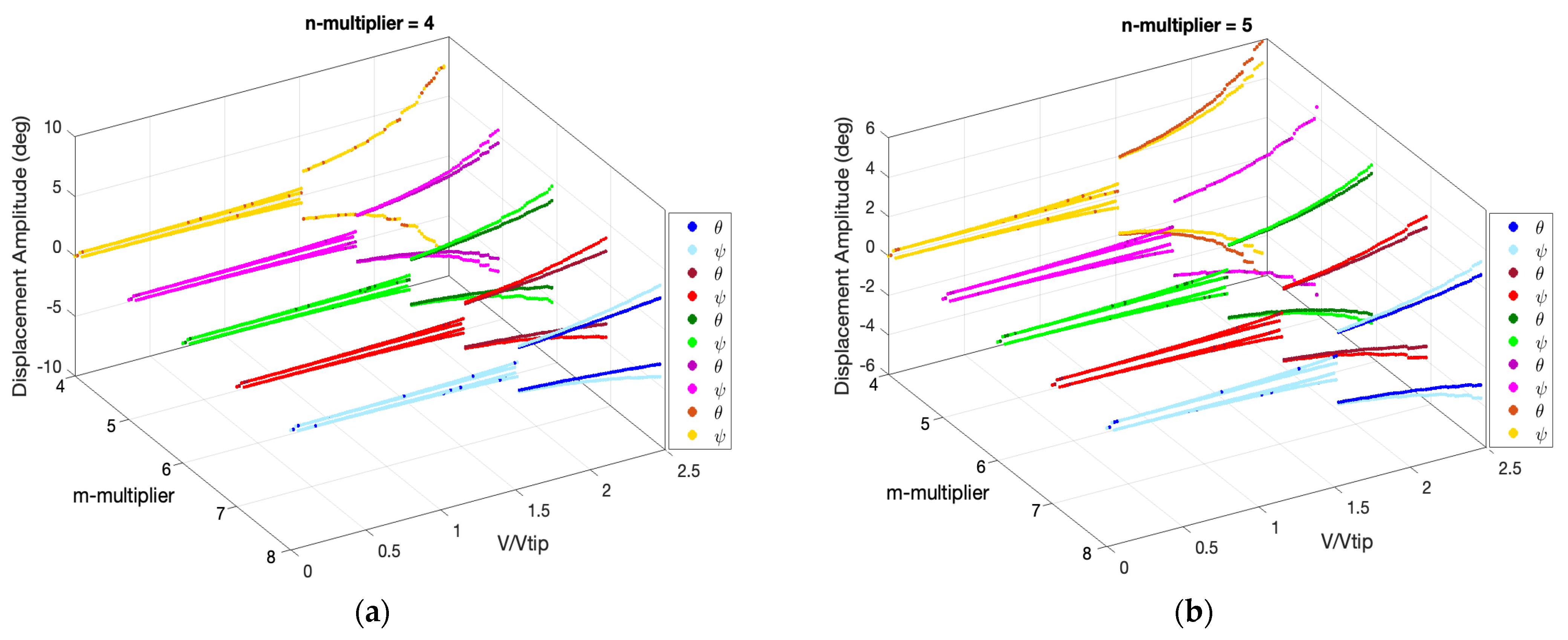
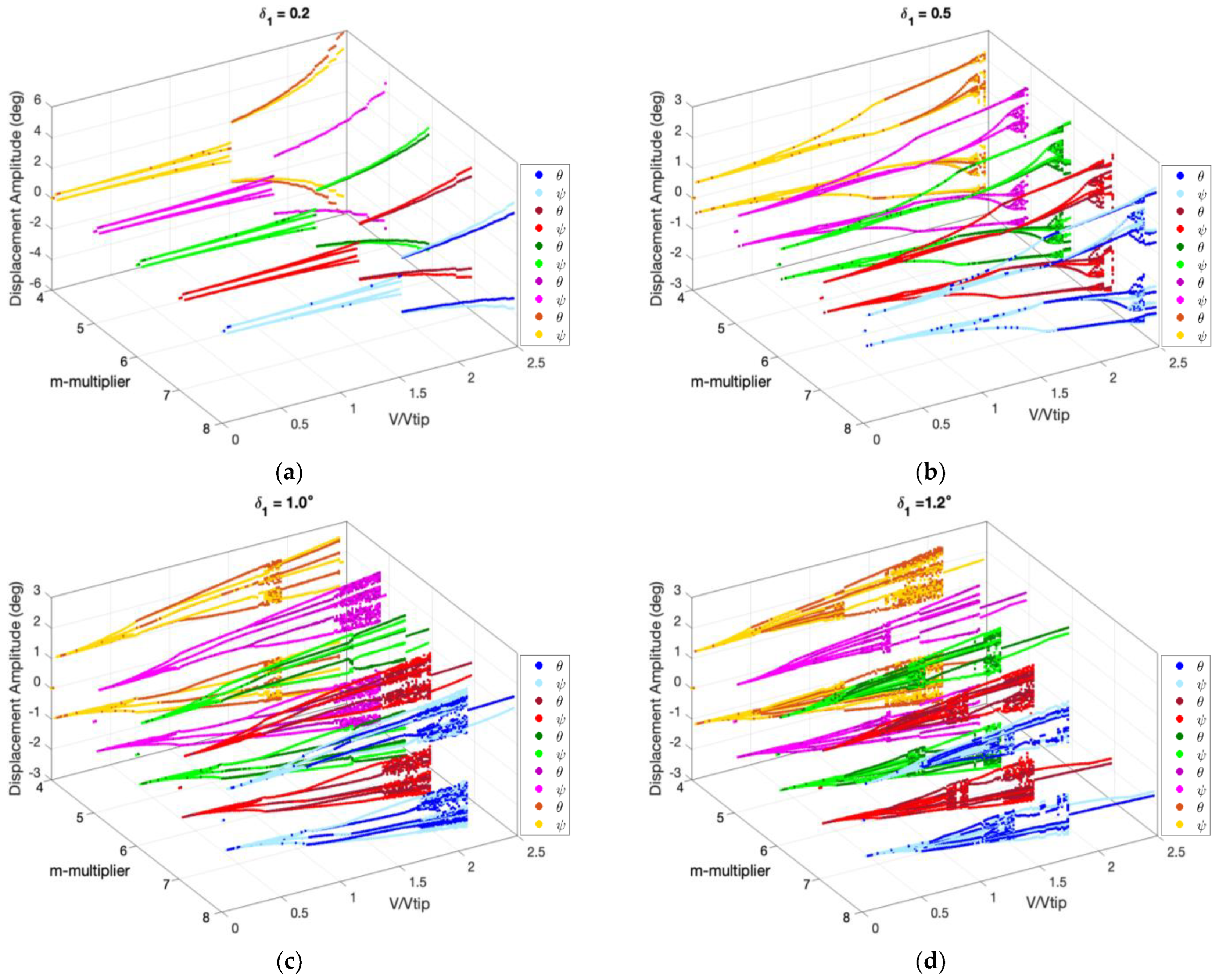
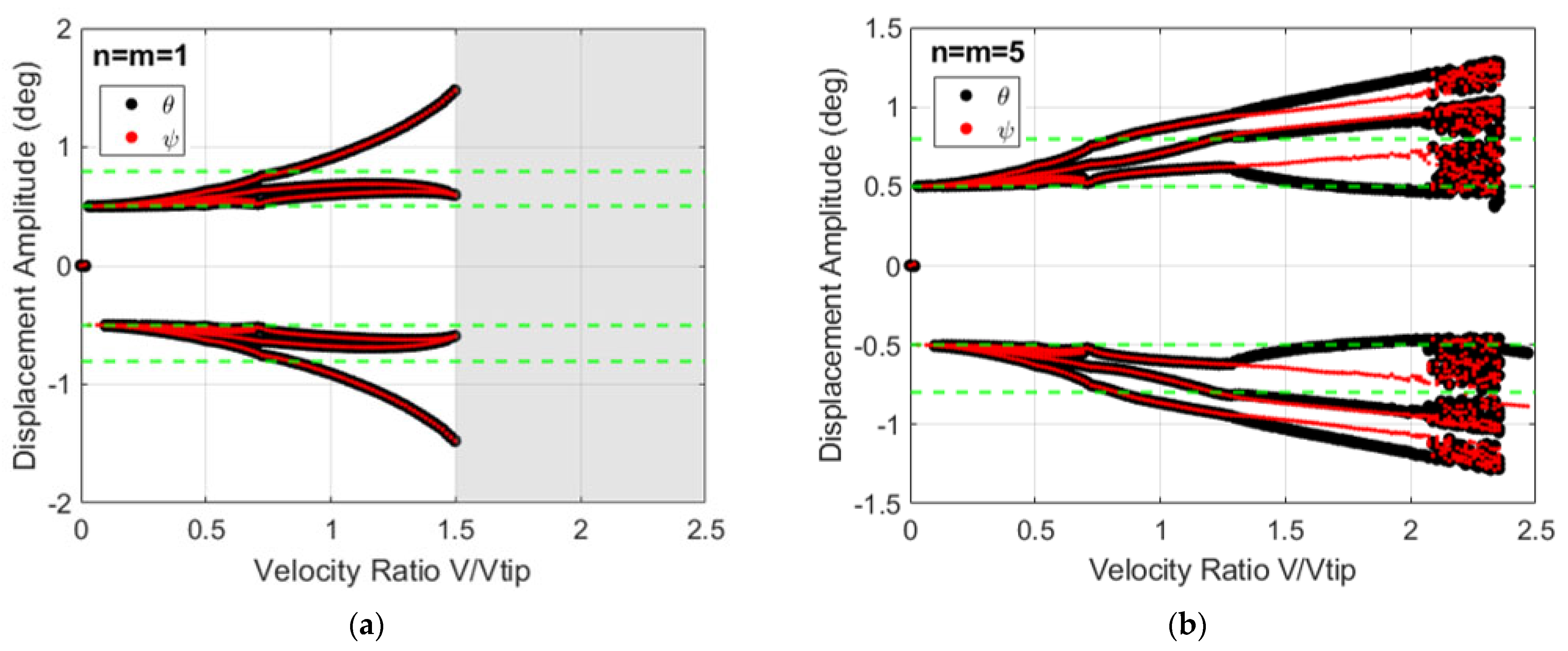
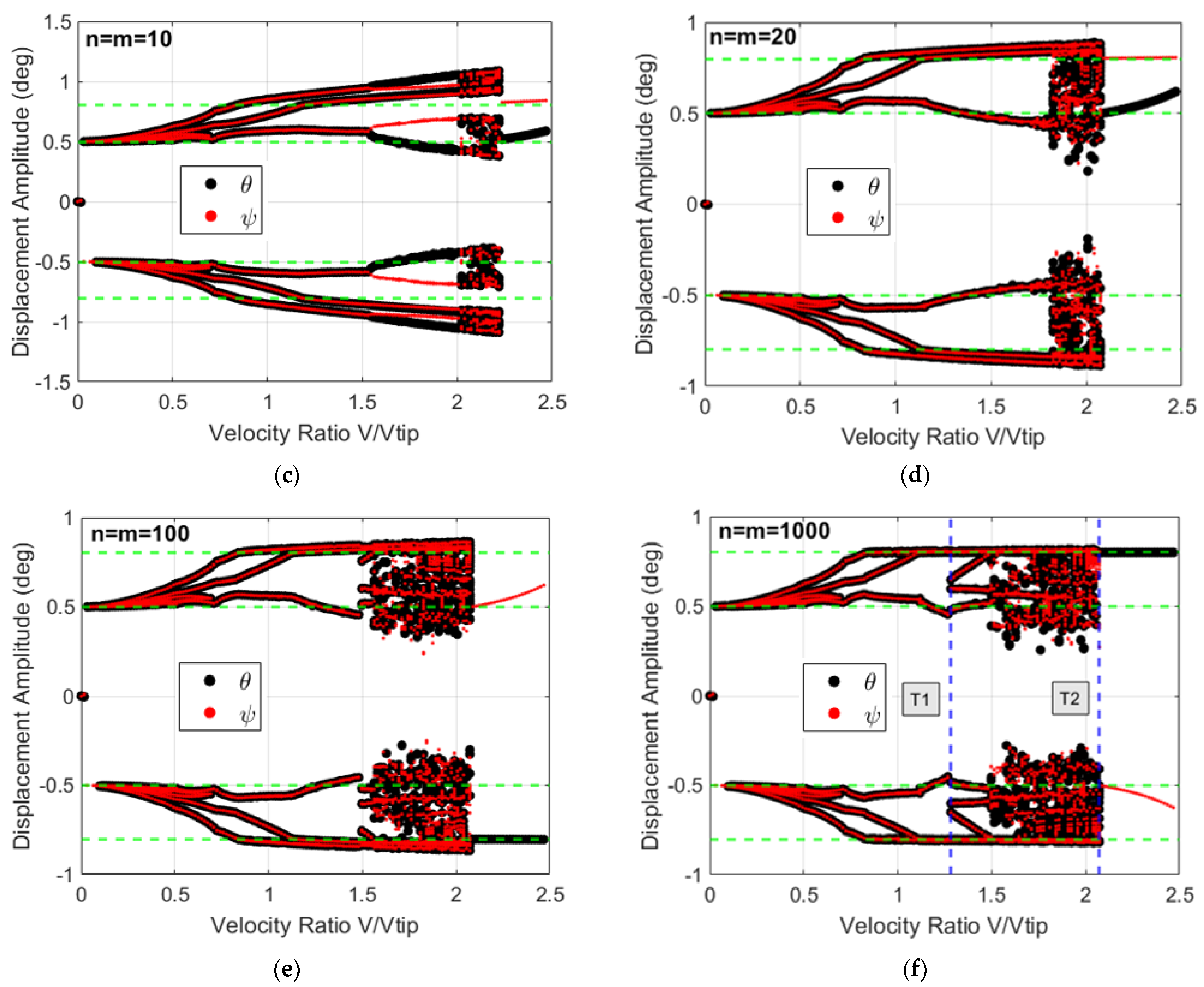
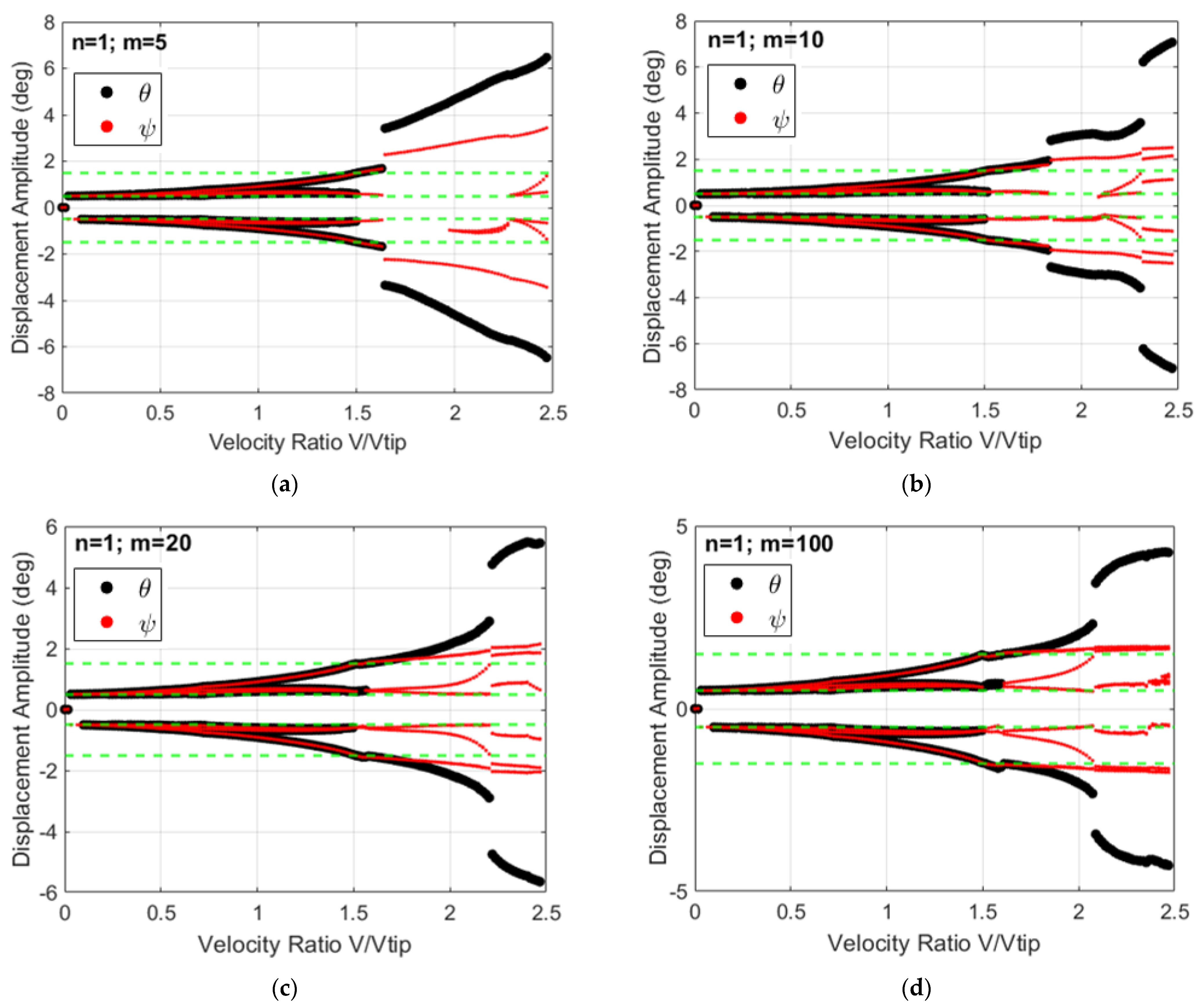
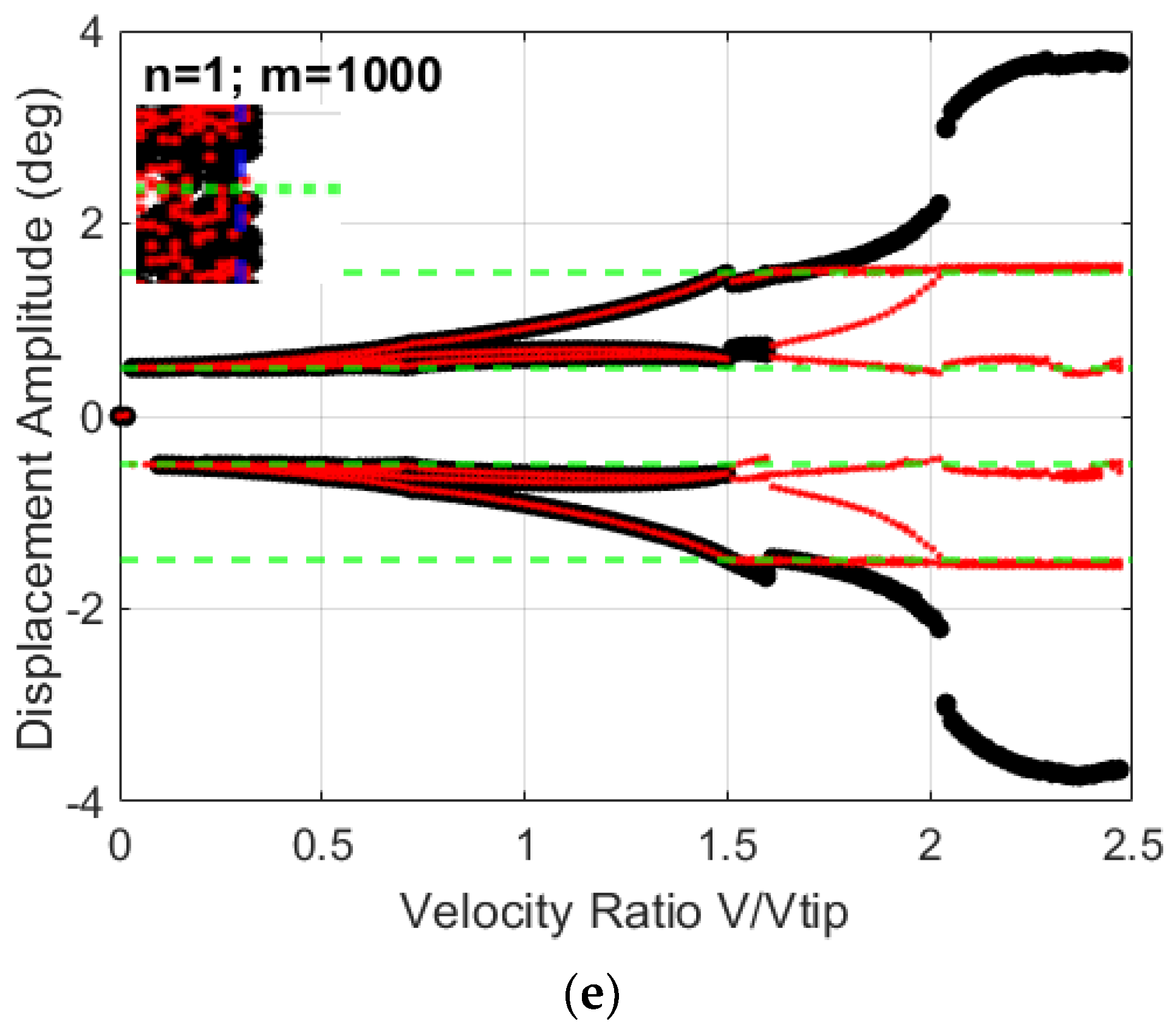
3.1. System Dynamics and Bifurcation Diagrams: Effects of Multi-Segmentation Properties

By incorporating multi-segmented freeplay, structural influences may induce aperiodic oscillations characterized by grazing bifurcations. Moreover, these findings reveal that the sticking phenomenon becomes noticeable under specific conditions and elevated freestream velocities, strongly influenced by the strength of the multi-segmented representation, gap sizes, and symmetry.

The characterization of a rotor-nacelle system which includes the complexities of both multi-segmented stiffness and gaps must be studied in portions. Therefore, it is important to outline each bifurcation diagram with varying stiffness multipliers for n and m, as well as unique ${\delta }_1$ and ${\delta }_2$ variables. The n variable will effectively change the strength of the structural stiffness beyond the ${\delta }_2$ boundary, but only for the pitch direction. Similarly, the m variable will effectively change the strength of the structural stiffness beyond the ${\delta }_2$ boundary, but only for the yaw direction. As the values for n and m increase, the structural stiffness subsequently increases, becoming more rigid. Varying the gaps ${\delta }_1$ and ${\delta }_2$ will alter when the new upper and lower limits of the piecewise stiffness function are initiated. The differences in the gap size dictates the onset of stiffness as the oscillations break through the gap threshold from the increasing in freestream velocities. In this section, three parameters are deeply investigated, namely, varying n with varying m, varying ${\delta }_2$ with varying m, and varying ${\delta }_1$ with varying m.

The first parameter studied in this section are the cases where the gap sizes ${\delta }_1$ and ${\delta }_2$ are fixed, with n and m stiffness multipliers are varied. For this investigation, ${\delta }_1=0.2°$, ${\delta }_2=1.5°$, m ranges from 4 to 8, and n ranges from 4 to 7, as shown in Figure 3a–d. The first characteristic of the bifurcation diagrams to note is an initial Hopf bifurcation near zero, followed by a second step increase in amplitude between a velocity ratio of 1.5 and 2. Furthermore, there seems to be period-adding behavior in all cases, with a clear hardening response in the system as n and m multipliers increase. Further investigation into these noteworthy behaviors will be studied in detail later. It should be mentioned that the result trends are similar in trends to cases with nonlinear freeplay, as the multi-segmented configuration is closely related to the nonlinear freeplay stiffness model when n = m = 1 [22].

The effects of the stiffness strength parameters n and m influence two main responses in the bifurcation. The first of these notable responses is in the amplitude when the m multiplier is increased. As shown in Figure 3a–d, by increasing the m multiplier in the first and fifth region of the yaw stiffness matrix, the overall oscillation with peak amplitudes in both pitch and yaw decay. When m increases, the resulting effects would be an increase in the hardening of the stopper, so the amplitude reduction shown in Figure 3 is exactly what we expect should happen. Furthermore, this effect also results in a switch of the dominant deflection angle (pitch amplitude is higher than yaw amplitude, to yaw amplitude is higher than pitch amplitude), when it passes from asymmetric (m < n) to symmetric (m = n) to asymmetric (m > n). The second effect is the variation between the $\theta$ and $\psi$ deflections when altering the n multiplier. Looking at one case from each plot, for instance when m = 4 shown in yellow and orange, as the n multiplier increases, there is a clear separation in the $\theta$ and $\psi$ displacement amplitudes.

To investigate the effects of the multi-segmented stiffness on the system’s dynamics, the gap ${\delta }_2$ and the strength of the stiffness in the yaw degree of freedom, m, are varied when keeping the strength of the stiffness in the pitch degree of freedom, n, and the gap ${\delta }_1$ equal to 5 and 0.5$°$, respectively. The corresponding bifurcation diagrams, shown in Figure 4a–d, illustrate ${\delta }_2$ decreasing from 1.5$°$ to 0.8$°$, with each plot increasing the m-multiplier from 4 to 8. In this study, there are many complex dynamical responses that become apparent as the strength of the stiffness in the yaw degree of freedom, m, increases. For instance, in Figure 4b, as the stiffness in the yaw degree of freedom increases, the response of the system causes the onset of possible chaotic and period-adding behaviors at lower freestream velocities. This investigation also illustrates the effect of decreasing the distance between ${\delta }_1$ and ${\delta }_2$. As ${\delta }_1$ approaches ${\delta }_2$, the complex aperiodic responses take place at lower freestream velocities with the possible presence of higher bifurcations, followed by rotor-nacelle locking or sticking to a fixed position in the pitch and yaw deflections, as shown in Figure 4d.

Next, the effects of the inner gap ${\delta }_1$ when varying the strength of the yaw degree of freedom, m, on the dynamical responses and bifurcations of the system are examined when keeping the values of the outer gap ${\delta }_2$ and the strength of the pitch degree of freedom equal to 1.5$°$ and 5°, respectively. The corresponding bifurcation diagrams for both the pitch and yaw angles are plotted in Figure 5 for various values of the inner gap ${\delta }_1$. Inspecting the plotted bifurcation diagrams in Figure 5, it is noted that when ${\delta }_1$ is approaching ${\delta }_2$, a reduction in the oscillating amplitudes is observed and the onset of complex regions occurs at lower freestream velocities. The most significant change caused by varying the ${\delta }_1$ gap is illustrated in the differences between Figure 5a and b. When the ${\delta }_1$ gap is far from the ${\delta }_2$ gap, three major characteristic changes occur: the prementioned decrease in amplitude, period-adding, and the introduction of a possible chaotic region at high freestream velocities considered in this investigation. Secondly, the influence of increasing the m-multiplier for the stiffness in the yaw degree of freedom results in a hardening response in the yaw direction. This hardening stiffness is then shown to affect the bifurcation of the yaw and pitch near the end of the simulation shown in Figure 5b–d.

As indicated in the plotted bifurcation diagrams in Figure 5, it is clear that the sticking phenomenon takes place when the ${\delta }_1$ gap is closer to the ${\delta }_2$ gap. Also, this phenomenon becomes more apparent and takes place at a lower freestream velocity when the strength of the multi-segmentation (m in this case) is larger. The question of what decides the direction in which pitch and yaw become fixed is pondered and hypothesized that the initial condition may influence this behavior. To fully understand the behaviors discussed, the time histories, phase portraits, frequency spectra, and basin of attraction studies are performed at key points of interest. The overall response of the system illustrated four key behaviors worthy of further investigation. The first is the possible chaos region at higher freestream velocities, as many of the bifurcation diagrams illustrate multiple points of oscillation at a single velocity (e.g., Figure 4c). Secondly, the cases where pitch and yaw deflections become fixed (sticking) in a particular orientation at high freestream velocities (i.e., Figure 5d). Third, there is a notable amplitude decrease with increased rigidity (Figure 3); this can also be seen when the ${\delta }_2$ gap limits are decreased with fixed ${\delta }_1$ (Figure 4), and ${\delta }_1$ gap limits are increased with fixed ${\delta }_2$ (Figure 5). Finally, further study is needed to understand the cause of the complex aperiodic behaviors in nearly all cases, and the oscillations around these points and the possible source of bifurcation. To this end, three cases are selected, studied, and characterized. Several transition points are chosen based on noteworthy portions of the bifurcation diagrams, and characterized using their time histories, phase portraits, and susceptibility to initial conditions. It should be mentioned that similar analyses and examinations can be performed to all studied bifurcation diagrams, however, for brevity only the most interesting transitions or scenarios are deeply investigated. Based on the resulting characterization, the physical limiting conditions applied to the system, and parameters assigned to those conditions, a clearer understanding of the physical system is provided and explained.

The following case is selected which has the given properties of ${\delta }_1=0.5°$, ${\delta }_2=0.8°$, $n=4$, and $m=6$. The corresponding bifurcation diagram for this configuration is illustrated in Figure 6. This case encompasses many interesting bifurcation behaviors, with the initial Hopf bifurcation followed immediately by period-adding, which transforms into separation in the pitch and yaw deflections as the lower branch crosses over the gap limit, continuing into a possible chaos region, and finally settling into a fixed axis in both pitch and yaw directions commonly known as the sticking phenomenon. Based on these behaviors, four transition points are selected as follows: T1 at velocity ratio 0.7, T2 at velocity ratio 1.2, T3 at velocity ratio 1.7, and T4 at velocity ratio 2.2. These four transition points are illustrated by the blue dashed lines with their respective title and are subsequently studied before and after each transition. The green dashed lines at $\pm 0.5°$ and $\pm 0.8°$ represent the upper and lower gap limits of ${\delta }_1$ and ${\delta }_2$, respectively.

This configuration’s bifurcation diagram shown in Figure 6 exhibits behaviors of period-adding, possible chaos, and fixed deflections. Only the results for the pitch degree of freedom are presented to avoid repetitive plots. The first method to characterize these possible behaviors is to investigate the time histories. The time history plots, illustrated in Figure 7a, represent the last three seconds of the simulation, for which the pitch before the transition is shown in black, the pitch after the transition is shown in red, and the green dashed lines represent the ${\delta }_1$ and ${\delta }_2$ gap limits. At the first transition point, T1, the oscillation at steady-state is dominated by the grazing contact of the ${\delta }_1$ gap limits. At increased freestream velocities, T2, the peak oscillations are dominated by the grazing contact as the primary peak transitions through the ${\delta }_2$ gap limits. At T3, the secondary peaks begin transitioning through the ${\delta }_2$ gap. It should be mentioned that the peak amplitudes and subsequent secondary oscillation are more prevalent at higher freestream velocities. However, at T4, the rotor-nacelle becomes fixed along the pitch and yaw directions corresponding to the ${\delta }_1$ and ${\delta }_2$ gap limits, where the pitch is fixed with the ${\delta }_1$ boundary and yaw is almost fixed with the ${\delta }_2$ boundary with the sticking phenomenon.

The phase portraits, shown in Figure 7b, capture the variability of the rotor-nacelle system as the freestream velocity increases. The phase portraits at the first point, T1, show a limit-cycle oscillation forming immediately beyond the ${\delta }_1$ gap boundary. At T2, the limit-cycle oscillation begins impacting the ${\delta }_2$ boundaries, and the resulting pitch and yaw deflections begin separating (i.e., they are not perfectly overlaying). At T3, multiple stability loops are created, with larger limit-cycle oscillation at the ${\delta }_2$ boundary. Moreover, the pitch and yaw deflections are showing aperiodic responses near the $0°$ deflection angle. Finally, at T4, the phase portraits illustrate a single point for the pitch and yaw deflections, fixed by the negative ${\delta }_1$ and ${\delta }_2$ limits, respectively.

The spectral frequencies, plotted in Figure 7c, effectively characterize the oscillations from the time histories. In the case of T1, at high frequencies, the resulting spectral amplitude decreases which can be seen at all points of interest. As for the pitch spectral density transition at T1, it is observed that the frequency increases as seen by the primary frequency before T1 at 1.03 Hz and after T1 at 1.61 Hz. At T2, the pitch deflection dominant frequencies before and after this selected transition remain relatively unchanged at lower frequencies. However, at larger frequencies, the frequency response of the system after T1 begin increasing compared to before T1. At T3, the system’s frequencies changes from clear dominant frequencies before the transition, to the presence of several frequencies after T3, which is a sign of aperiodicity after this transition. The final transition, T4, shows a much larger aperiodic response before the transition with transitioning to the sticking scenario with only the primary peak frequency being clearly defined.

The subsequent analyses focus on the pseudo-phase portraits pertaining to the pitch response. The pseudo-phase portraits, depicted in Figure 8, present the deflection angle, α(t), in relation to two time-shifted deflection angles, $\alpha \left(t+\mathsf{{\rm T}}\right)$ and $\alpha \left(t+2\mathsf{{\rm T}}\right)$, with ${\rm T}=1/3$ s. These time-shifted histories serve as proxies for angular velocity and angular acceleration, facilitating the computation of a Poincaré map, which is essential due to the autonomous nature of the rotor-nacelle system. The Poincaré map is an indicator of the periodicity/aperiodicity of the system response [28]. Namely, a Poincaré map consisting of a finite number of discrete points N is periodic, with period number N; a continuous closed loop denotes a quasiperiodic response; and an infinite set of points not making a closed loop, and often resulting in a fractal shape, denotes a chaotic motion. Subsequently, the Poincaré map identifies the points on the plane where $\alpha \left(t+2\mathsf{{\rm T}}\right)=0$ while $\alpha \left(t+\mathsf{{\rm T}}\right)>0$ is satisfied. Based on Figure 8, the Poincaré map is used to study the rotor-nacelle system’s response at the velocity ratio of 1.97 due to the strong aperiodicity in this region. The resulting Poincaré map, shown in Figure 8, depicts the presence of infinite points that do not close a loop and hence the chaotic behavior of this system at this velocity ratio. Similar responses are obtained in the range of velocity ratios after transition T3 and before transition T4, showing the aperiodicity of the rotor-nacelle system. Other indicators of chaos are also available, such as the largest Lyapunov exponent of the response. Only Poincaré maps are used for the rest of this work, but a case study using the largest Lyapunov exponent on Figure 8 was also performed using a code by Wolf et al. [29]. The system at the velocity ratio of 1.97 has a largest Lyapunov exponent of 12.1432, again confirming that the response is chaotic.

The basin of attraction study investigates the four points of interest illustrated in Figure 9a–d. The four points of interest selected are at the velocity ratios of 0.7, 1.2, 2.1, and 2.4 because of the behaviors witnessed at these locations in Figure 6. The first plot, Figure 9a at the velocity ratio 0.7, is selected at a low velocity point with grazing contact behavior observed. At this point, Figure 9a shows that the initial conditions do not play a significant influence in how the system will respond. With increased freestream velocity, a second basin of attraction study is performed at 1.2, as shown in Figure 9b. In this region, the system begins forming the bounds of a patterned effect of the initial conditions. The third basin of attraction study point selected is at 2.1, with the results illustrated in Figure 9c. The fourth case, depicted in Figure 9d, is considered at the velocity ratio of 2.4. At both 2.1 and 2.4, there are clearly defined boundaries, with higher amplitude regions outlined. In both cases, the initial conditions can affect how the system will oscillate at these higher freestream velocities among three different possible solutions.

This configuration was selected based on its unique bifurcation characteristic of period adding, possible chaos, and sticking phenomenon. The results of this case showed that the ${\delta }_1$ and ${\delta }_2$ gap creates a grazing contact from which grazing bifurcations are induced. As the freestream velocities are increased and grazing contact is achieved, the bifurcation diagrams depict aperiodicity and variability in the pitch and yaw directions. Finally, at a critical point, the system’s behavior transitions from chaos to lock the pitch and yaw along the negative pitch and yaw directions. The direction in which the pitch and yaw deflections become locked to, as well as the amplitudes within the chaos region, are highly dependent upon the initial conditions.

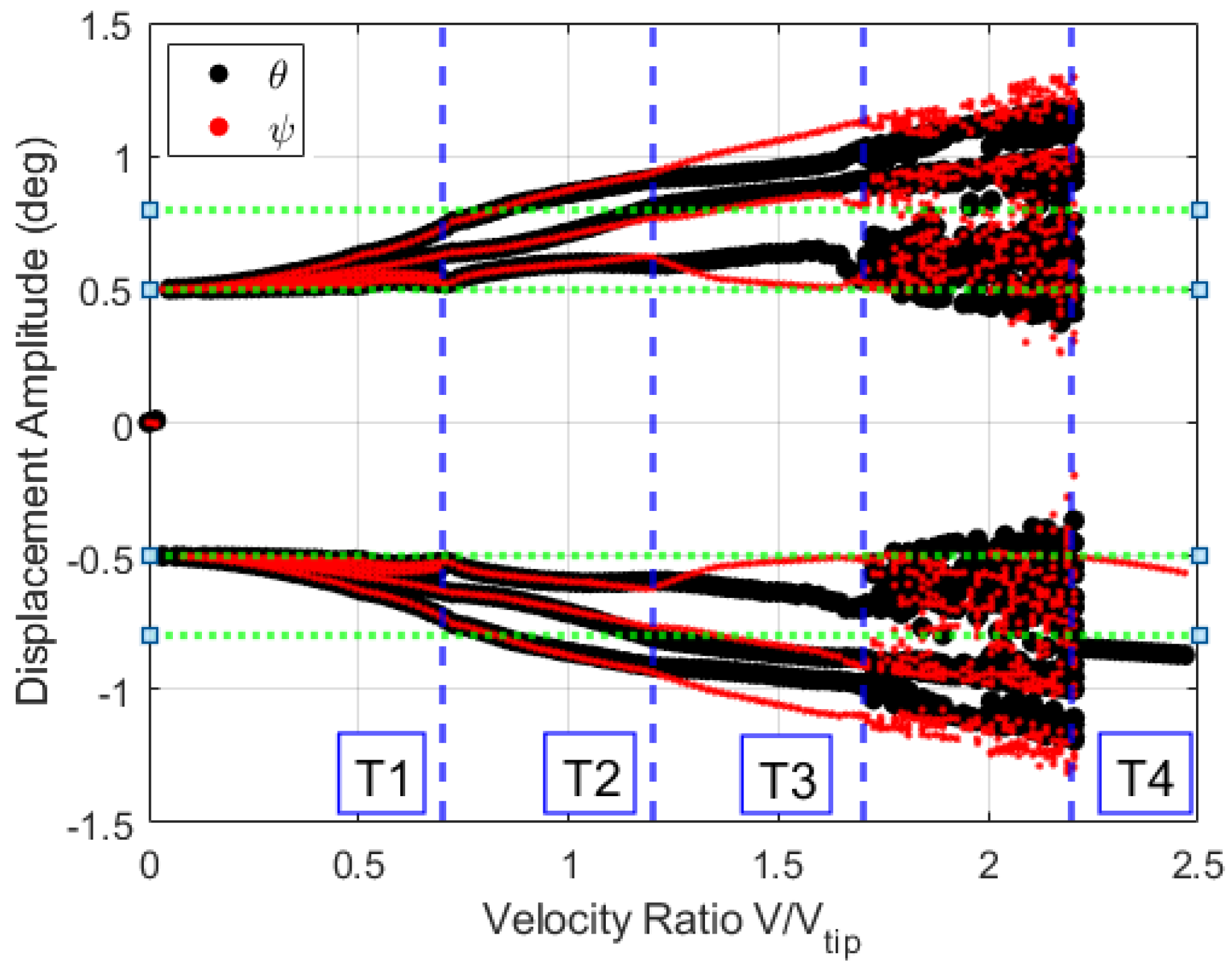
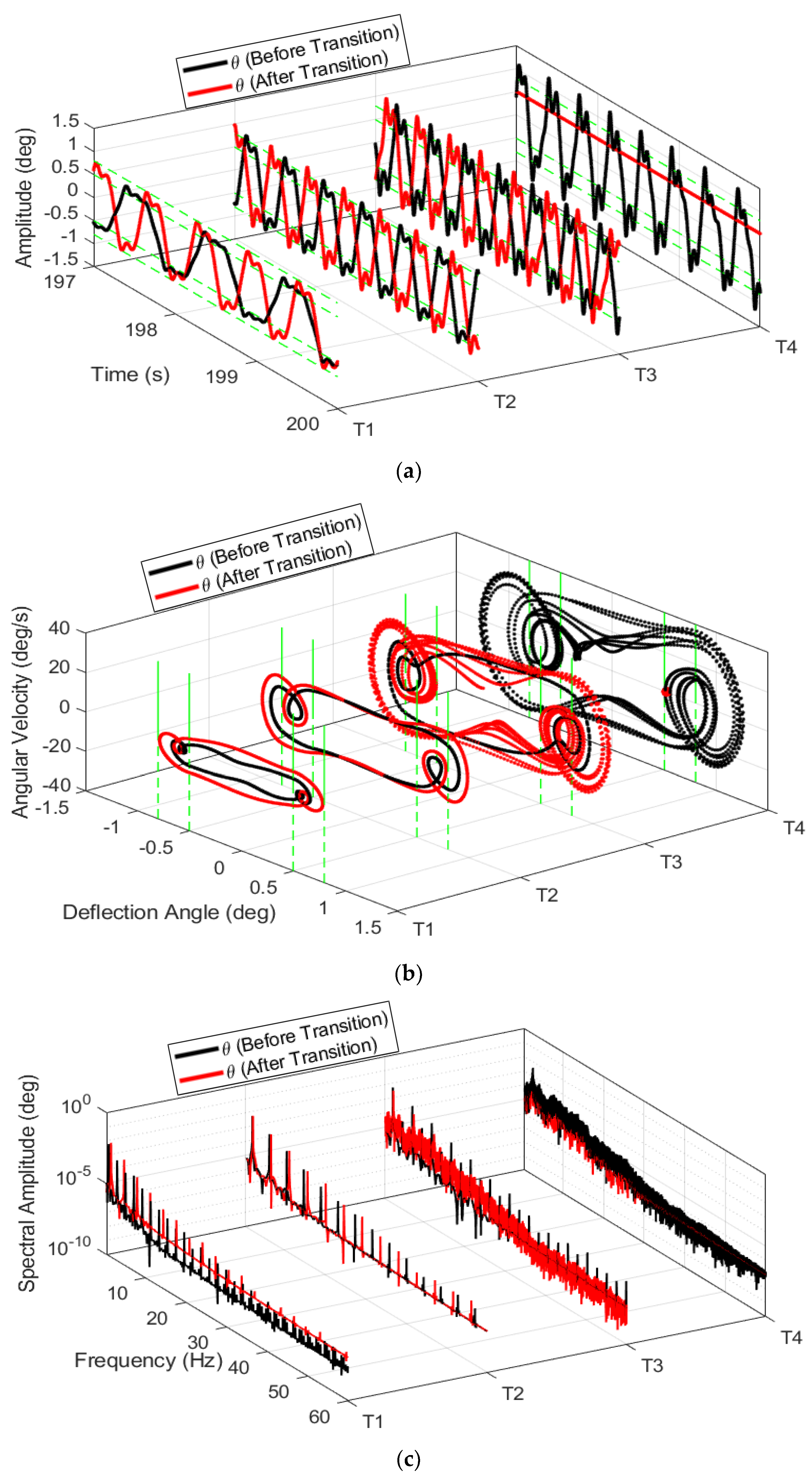
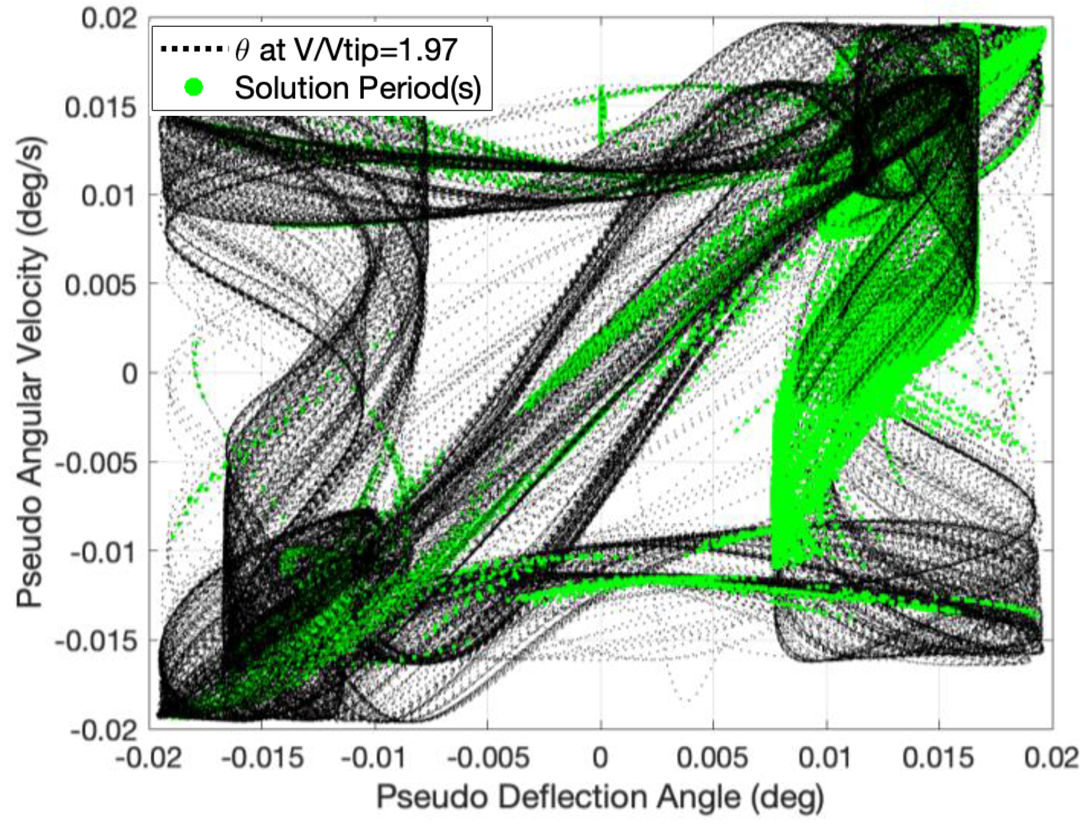
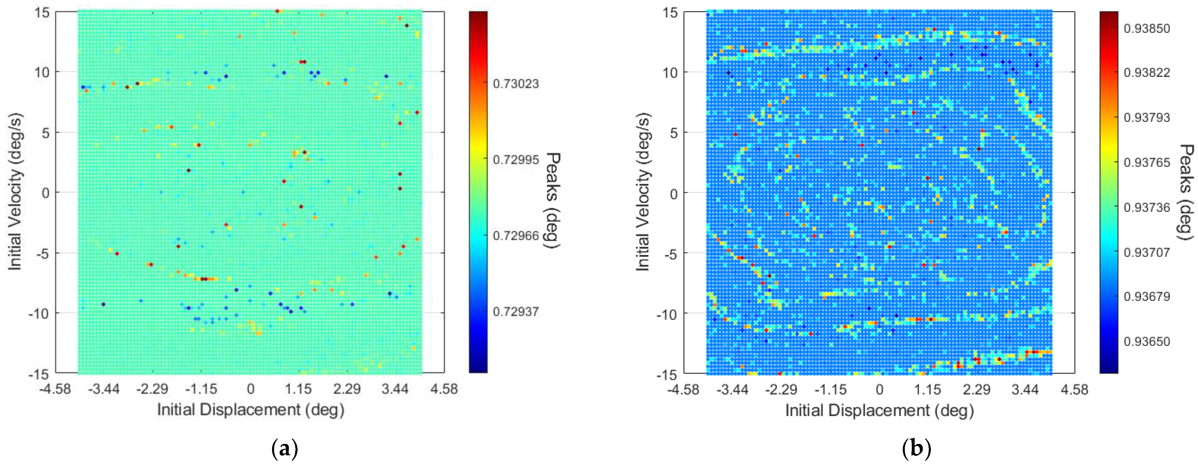
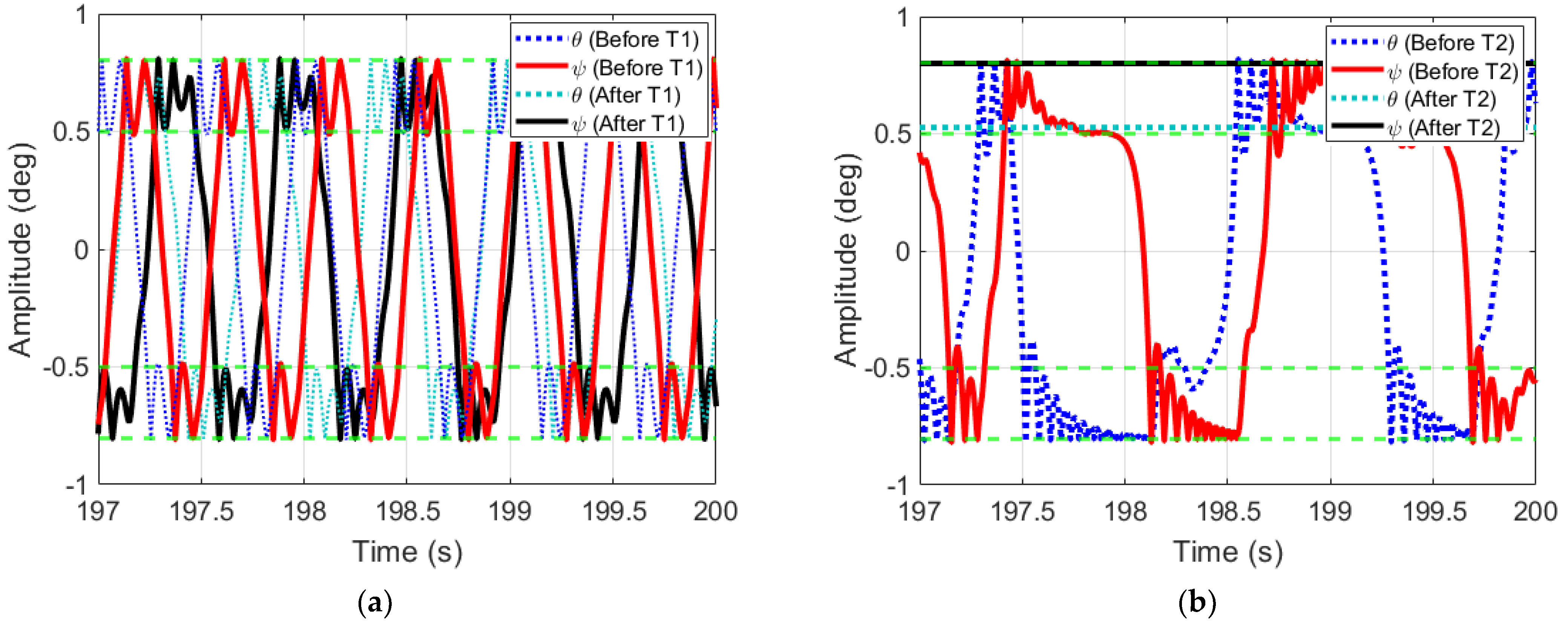
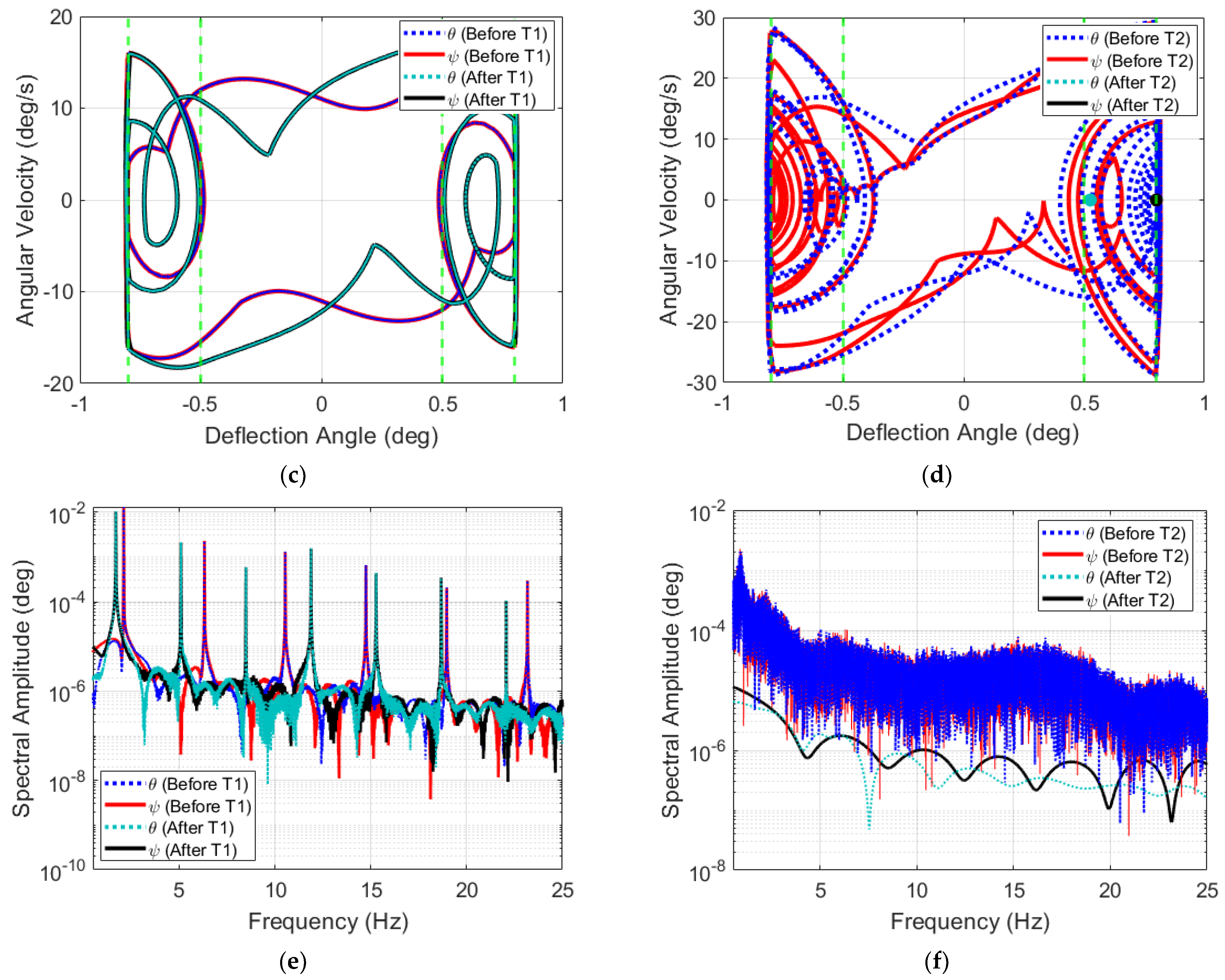
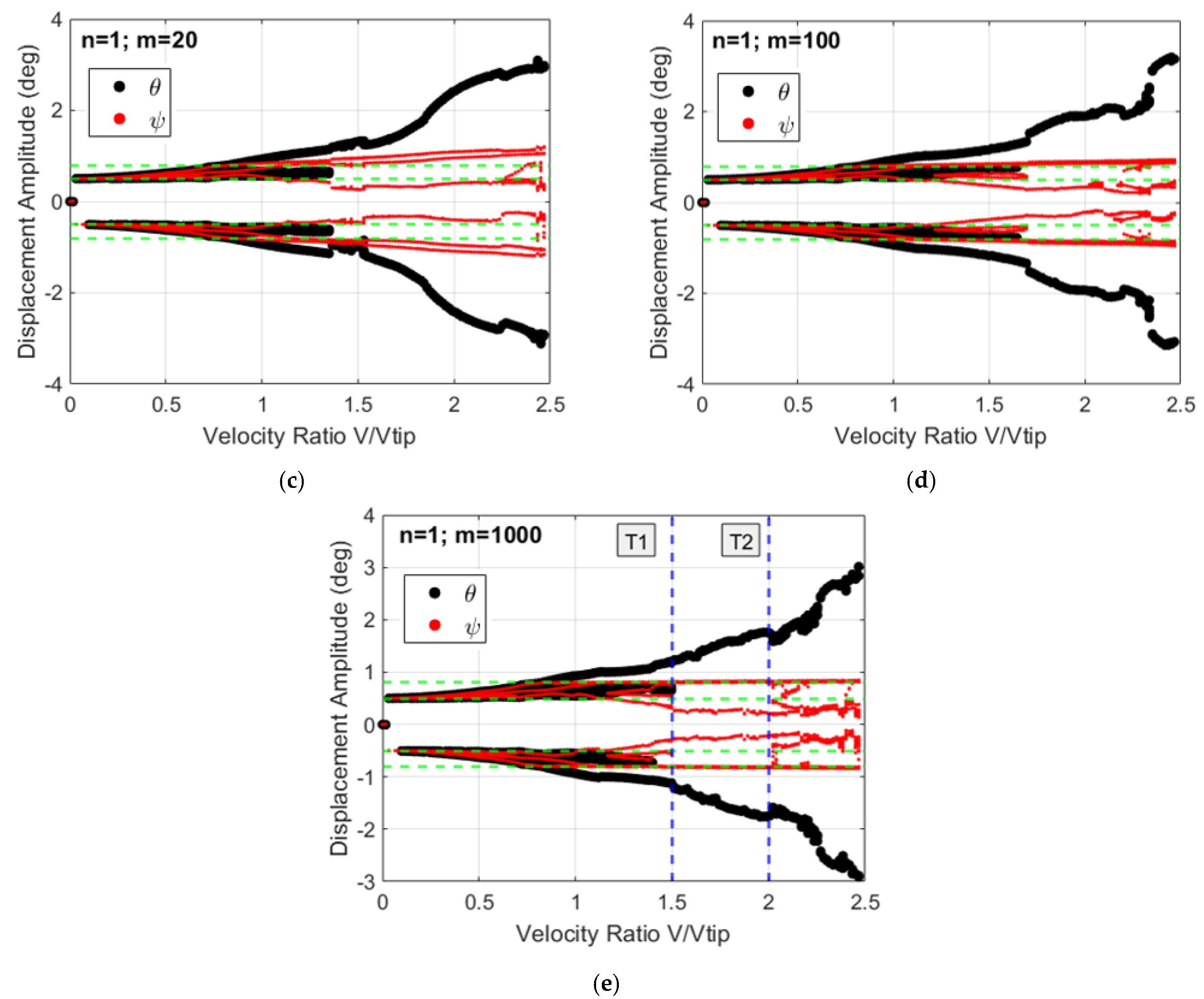
3.2. System’s Dynamics and Bifurcation Diagrams: Route to Impact

Expanding upon the concept of symmetric and asymmetric application of the n and m stiffness multipliers, pitch and yaw, respectively, this portion of the research outlines the route to impact. The goal of this analysis is to investigate the effects of increasing the strength of the multi-segmented stiffness to the point of near rigidity. As the values are increased, the resulting stiffness matrix will act as a solid impact on the system, and a study into the bifurcation response will take place. Furthermore, in two cases, an analysis and characterization of key transition points are studied. Lastly, this study investigates any relationship between the aperiodic region and sticking phenomenon with respect to the strength of multi-segmented stiffnesses and gaps.

In order to accomplish this, the following multi-segmented stiffnesses in the pitch and yaw degrees of freedom where n = m for various values are considered. In this configuration, depicted in Figure 10a,b, the black, blue, cyan, magenta, red, and green lines represent the cases where n and m equal 1, 5, 10, 20, 100, and 1000, respectively. Furthermore, the four dashed lines represent the ${\delta }_1$ and ${\delta }_2$ gap limits. As n and m increased, the resulting slopes in the first and fifth region approaches a vertical line, or physically a rigid impact. It should be mentioned, at this stage, that the cases of n and m equal to 100 and 1000 almost have the same structural moments and hence the system’s bifurcation diagrams may not be influenced by this change from 100 to 1000. Additionally, it should be noted that the case of n and m equal 1 is the classical freeplay nonlinearity scenario. Applying these various model conditions to the symmetric and asymmetric scenarios, this study can outline the route to impact and how the rotor-nacelle system’s response is affected by this.

3.2.1. Symmetric Configuration for Multi-Segmented Rotor-Nacelle System

This section considers the symmetric scenario of the stiffness multipliers for pitch (n) and yaw (m) for two configurations. The first configuration considered is shown in Figure 10a when ${\delta }_1$ = 0.5$°$ and ${\delta }_2$ = 1.5$°$, and the second one is presented in Figure 10b when ${\delta }_1$ = 0.5$°$ and ${\delta }_2$ = 0.8$°$. In both configurations, six symmetric stiffness multipliers are applied such that n and m equal: 1, 5, 10, 20, 100, and 1000. As the stiffness multipliers increase, the resulting contact with the ${\delta }_2$ gap becomes more rigid and starts to represent a wall condition leading to impact. This effect is illustrated and described in Figure 10. Moreover, by considering the larger ${\delta }_2$, the system will be free to oscillate with the effects from ${\delta }_1$ boundary for wider range. Then, by decreasing the ${\delta }_2$ gap, the system becomes more susceptible to the impact effects of the ${\delta }_2$ gap from smaller oscillation amplitudes and hence at lower freestream velocities.

As illustrated in Figure 11a–f, the bifurcation diagrams of the pitch and yaw degrees of freedom for the symmetric configuration when ${\delta }_1$ = 0.5$°$ and ${\delta }_2$ = 1.5$°$ are shown. When n and m equal 1, a classical freeplay nonlinearity case, a grey region is depicted because the system’s response diverges as it crosses the flutter speed; showing that in this case, whirl flutter coincides with the grazing contact. It is interesting to note the effects of the gap limits in this case, immediately preceding this grey region. In fact, at the velocity ratio of roughly 1.5 in all cases, the gap limits influence the oscillations of the system. At this point, the rotor-nacelle system transitions from a period-3 to period-2 response (focusing on the number of peak values in the bifurcation diagram), as shown in Figure 11b–f. Furthermore, at higher velocities, one of the branches of the system’s response undergoes a period doubling within the gap limits of ${\delta }_1$ and ${\delta }_2$. For instance, this can be seen in Figure 11b at a velocity ratio of roughly 1.7. There is also a notable region at high velocities with strong aperiodicity. For example, in Figure 11b, this region begins at a velocity ratio of roughly 2.4. Interestingly, as stiffness multipliers are increased, this region is forced to initiate at lower freestream velocities. This can be witnessed when comparing Figure 11b against Figure 11d, where this region begins at a velocity ratio of roughly 2.1. These regions are defined in

Table 2. Regions of interest for the two scenarios: (1)${\delta }_1$ = 0.5$°$ and ${\delta }_2$ = 0.8$°$ and (2)${\delta }_1$ = 0.5$°$ and ${\delta }_2$=$1.5°$).

	Strong Aperiodicity Range $({\mathit{\delta }}_1=0.5° \mathbf{and} {\mathit{\delta }}_2=1.5°)$	Strong Aperiodicity Range $({\mathit{\delta }}_1=0.5° \mathbf{and} {\mathit{\delta }}_2=0.8°)$	Sticking Phenomenon $({\mathit{\delta }}_1=0.5° \mathbf{and} {\mathit{\delta }}_2=0.8°)$
n= m = 1	$-$	$-$	$-$
n= m = 5	2.31–2.47 (0.16)	2.07–2.37 (0.30)	2.37–2.47 (0.1)
n= m = 10	2.17–2.47 (0.3)	2.02–2.22 (0.20)	2.22–2.47 (0.25)
n= m = 20	2.08–2.47 (0.39)	1.82–2.07 (0.25)	2.07–2.47 (0.4)
n= m = 100	2.02–2.47 (0.45)	1.49–2.07 (0.58)	2.07–2.47 (0.4)
n= m = 1000	1.99–2.47(0.48)	1.49–2.07 (0.58)	2.07–2.47 (0.4)

.

Furthermore, it follows from the bifurcation diagrams shown in Figure 11 that as the stiffness multipliers n and m are increased, there is a clearly defined transition in the system’s response around the ${\delta }_2$ gap limits. At low stiffness multipliers, the bifurcation branches are moderately influenced by the increase stiffness after crossing the ${\delta }_2$ gap limits, as shown in Figure 11b–d. However, at very high stiffness multipliers, these gap limits act as rigid constraints and cause an impact with the bifurcation branches, as indicated in Figure 11e,f. At these high values, as the system oscillates and attempts to cross over the ${\delta }_2$ gap, an impact will occur resulting in the behavior witnessed in the last two Figure 11e,f. Inspecting the bifurcation diagrams, it should be mentioned that the similarity of the pitch and yaw angles is broken as the strength of the multi-segmented stiffness is increased. This is particularly true at higher freestream velocities and when n and m are higher than 20.

The second scenario, when ${\delta }_1$ = 0.5$°$ and ${\delta }_2$ = 0.8$°$, is illustrated in Figure 12a–f. This scenario is similar to the previous one, in that the stiffness multipliers are both symmetrically applied and they are bounded by ${\delta }_1$ and ${\delta }_2$. However, they are vastly different in the limited region between gaps that factors into how the systems oscillations will respond. The most notable difference in this scenario, compared to the previous one, develops from the resulting sticking phenomenon shown at the end of each simulation in Figure 12b–f. At high freestream velocities, the pitch and yaw oscillations caused by the whirl flutter become locked to a particular side. For instance, in Figure 12b, both the pitch and yaw experience the sticking phenomenon at a velocity ratio of roughly 2.4 at which point they become locked into a negative displacement amplitude. Furthermore, this sticking can be seen to occur at lower and lower velocities ratios as the stiffness multipliers are increased. The exact regions of the strong aperiodicity and onset of the sticking phenomenon are outlined in Table 2. It should be mentioned that the bifurcation diagrams for the cases of n and m equal to 100 and 1000 have some discrepancies at higher velocities and when the impact effect takes place although the aperiodicity range is similar, however, the bifurcations are not exactly the same.

Table 2 outlines the regions of strong aperiodicity in both scenarios, and the onset velocity ratios of the sticking phenomenon in the scenario where ${\delta }_1$ = 0.5$°$ and ${\delta }_2$ = 0.8$°$. The table shows that for the case of ${\delta }_1$ = 0.5$°$ and ${\delta }_2$ = 1.5$°$, when increasing the stiffness multipliers, the region of strong aperiodicity increases while initiating at lower freestream velocities. Furthermore, for the case of ${\delta }_1$ = 0.5$°$ and ${\delta }_2$ = 0.8$°$, the strong aperiodicity region and the onset of sticking phenomenon are linked. At all n and m values for this case, the region of strong aperiodicity is followed by the sticking phenomenon. Due to these results, it can be logically assumed that for the case of ${\delta }_1$ = 0.5$°$ and ${\delta }_2$ = 1.5$°$, if the velocities are allowed to increase, a similar sticking phenomenon would ensue.

Further analysis and characterization is performed for the symmetric scenario when high values of the pitch and yaw stiffnesses’ multipliers (n = m = 1000) are considered. This case corresponds to the bifurcation diagrams shown in Figure 12f and two points of interest are selected, namely, T1 at 1.3 and T2 at 2.1. At these points, there is a transition in the behavioral response of the system. At T1, the inner branch intercepts the ${\delta }_1$ gap limits which cause period adding to occur. Moreover, at T2, the system transitions from a region of strong aperiodicity to the sticking phenomenon. To properly examine the characteristics of the rotor-nacelle system at these transition points, the time histories, phase portraits, and frequency domains are utilized before and after each transition occurs. For T1, the characteristics are studied at the velocity ratio of 1.2 and 1.4, and for T2, the characteristics are explored at the velocity ratio 2.0 and 2.2.

The time histories of the system, shown in Figure 13a,b, present the pitch dynamics preceding and following the transition event using distinctive line styles. Additionally, the figures display the multi-segmented gap limits, which are represented by green dashed lines situated at 0.5° and 0.8°, respectively. In the first case, Figure 13a for T1, the peak values experience grazing contact both before and after for pitch and yaw deflections. The time history plot at T2, illustrated in Figure 13b, shows a consistent trend for pitch and yaw for the before and after responses. For instance, both pitch and yaw before T2 are bounded by the ${\delta }_1$ and ${\delta }_2$ gap limits, with multiple oscillation between this region. Then after T2, both pitch and yaw experience the sticking phenomenon, becoming fixed to the positive ${\delta }_1$ and ${\delta }_2$ gap limits, respectively.

In the second characteristic study, the phase portraits at T1 and T2 are analyzed and are depicted in Figure 13c,d. At the first transition T1, Figure 13c, the effects of the multi-segmented gap and high stiffness multipliers become clear. In this case, both before and after T1, the phase portraits are severely bounded by the ${\delta }_2$ gap shown at the deflection angle $\pm 0.8°$. Furthermore, before T1, a single limit cycle oscillation is present, which then transitions into multiple limit cycle oscillations. In the second case, for T2, shown in Figure 13d, the influence of the ${\delta }_2$ gap continues to show at the deflection angle $\pm 0.8°$. However, as the system transitions through T2, the pitch and yaw become fixed with the positive ${\delta }_1$ and ${\delta }_2$ gap limits. In combination with the time histories, these results indicate the strong influence of the multi-segmented gaps and the rigid impact from the high stiffness in region I and V. It should be mentioned that a grazing-sliding bifurcation may take place due to the impact at high boundary.

The final characteristic study investigates the frequency domain, illustrated in Figure 13e,f, for T1 and T2, respectively. At the transition point, T1, depicted in Figure 13e, the frequency for pitch and yaw decrease from before to after the transition. Moreover, before T2, as depicted in Figure 13f, multiple oscillations in the time history result in a noisy frequency response. It can also be witnessed, that after T2, the frequencies amplitudes and peaks become lowered as the pitch and yaw deflections experience the sticking phenomenon.

3.2.2. Asymmetric Configuration for Multi-Segmented Rotor-Nacelle System

The following investigation considers the asymmetric scenario of the stiffness multipliers where the pitch degree of freedom is less limited than the yaw one. In these configurations, the n multiplier is fixed to 1, and the m multiplier is varied such that m equals 5, 10, 20, 100, and 1000. Furthermore, as in the symmetric configurations, the two scenarios considered are when ${\delta }_1$ = 0.5$°$ and ${\delta }_2$ = 1.5$°$, and when ${\delta }_1$ = 0.5$°$ and ${\delta }_2$ = 0.8$°$. It should be mentioned that both the pitch and yaw motions are plotted to study the coupled response of the system where pitch is shown in black and yaw in red. Lastly, the gap limits of ${\delta }_1$ and ${\delta }_2$ are represented by the green dashed lines.

The first scenario, ${\delta }_1$ = 0.5$°$ and ${\delta }_2$ = 1.5$°$, is depicted in Figure 14a–e. The asymmetric application of stiffness multipliers illustrates the coupled influence between the pitch and yaw degrees of freedom, and the resulting oscillations caused from the asymmetric application of stiffness beyond the ${\delta }_2$ gap. The influence of the yaws’ higher m stiffness multiplier conversely affects the pitch deflection with the lower n stiffness multiplier due to the coupling of the rotor-nacelle system. For instance, in Figure 14a–c, at roughly the velocity ratio of 2.4, the higher stiffness yaw deflections begin interacting with the ${\delta }_2$ gap which in turn causes the pitch to undergo a transition. Furthermore, this same interaction can be observed in Figure 14d,e, at roughly the velocity ratio of 2.1. It can be noted from the bifurcation diagrams in Figure 14, that an increase in the yaw multi-segmented stiffness leads the pitch transition to take place at lower freestream velocities with the presence of sudden jump and this transition is directly connected to the interaction between the yaw motion and its higher gap limit. Inspecting the bifurcation diagrams in Figure 14, it is clear that there is grazing or/and grazing-sliding contact when the freestream velocity is increased. As for the grazing contact, this can be seen in all cases around the velocity ratio of 1.5, where the yaw deflections are interacting with the gap limit shown by the green dashed line. Concerning grazing-sliding contact, it may take place near a velocity ratio of 1.5 and 2 for the cases of multi-segmented yaw stiffness with ratios of m = 100 or 1000, as illustrated in Figure 14d and 14e, respectively.

Next, the asymmetric scenario of ${\delta }_1$ = 0.5$°$ and ${\delta }_2$ = 0.8$°$ is illustrated in Figure 15a–e. This scenario reinforces the previous asymmetric coupling seen with ${\delta }_1$ = 0.5$°$ and ${\delta }_2$ = 1.5$°$. The influence from the high stiffness in the yaw, directly impacts the pitch deflection as result of the grazing contact or/and grazing-sliding contact. This is depicted at several points where the red line crosses the green dashed line, and a subsequent response in the pitch can be seen even through the pitch had crossed the gap limit much earlier. For example, in Figure 15d, when n and m are equal to 1 and 100, respectively, at a velocity ratio of roughly 2.25, the yaw oscillations contact the gap limits and a notable drop in the pitch deflection is recorded. Due to this coupling, as the yaw stiffness multiplier increases, the pitch deflection is subsequently controlled and several bifurcations take place. It should be mentioned that the asymmetry in the multi-segmentation representation results in a disappearance of the sticking phenomenon for the range of freestream velocities considered in this study. This is due to the consideration of the classical freeplay configuration for the pitch degree of freedom.

To better understand the underlying behaviors observed in the asymmetric configuration results, the time histories, phase portraits, and spectral frequency densities are plotted and examined before and after transition points T1 and T2, as illustrated in Figure 15e. T1 is considered at a velocity ratio of 1.5 and T2 at 2. The plots in Figure 16 depict the characteristics of the transitions before and after such that at T1 is studied at the velocity ratios of 1.4 and 1.6, and T2 at 1.9 and 2.1. In these subfigures, the pitch before the transition event is represented by the blue dotted line and after with a dark cyan dotted line, and the yaw before is represented with the red solid line and after with a black solid line. As for the multi-segmented gap limits, they are represented by the green dashed lines at 0.5$°$ and 0.8$°$.

The first study investigates the time history plots before and after T1, as shown in Figure 16a. In this case, the yaw motion experiences grazing or/and grazing-sliding contact as the primary and secondary peaks of black and red lines are bounded within the ${\delta }_1$ and ${\delta }_2$ gap limits. The pitch is dominated by a primary peak, which is not shown to be influenced by the gap limit as in the yaw motion. At the transition T2, indicated in Figure 16b, a similar trend is witnessed. However, the yaw before and after the transition changes from having two peaks to having three. Moreover, the yaw motion undergoes a grazing or/and grazing-sliding contact as it is bound by the ${\delta }_1$ and ${\delta }_2$ gap limits. Finally, the pitch degree of freedom has oscillated with larger deflection amplitudes compared to the previous transition point.

The second investigation looks into the phase portraits of the system with the previously stated configuration illustrated by Figure 16c,d for T1 and T2, respectively. In the case before and after T1, Figure 16c, the yaw motion is confined by the ${\delta }_2$ gap limits at $\pm 0.8°$. Furthermore, before T1, the system undergoes multiple limit cycle oscillations, then after T1, the system transitions to a single limit cycle oscillation. The pitch is shown to have notable dip both before and after the ${\delta }_2$ gap limits at a velocity ratio of roughly 1.4 before T1 and 1.6 after T1 which is influenced by the yaw motion. A similar response is witnessed before and after T2. However, higher angular velocities are reached, and the limit cycle oscillation before T2 results in more limit cycle oscillations compared to T1. In comparison with the time history analysis, the system is shown to be dominated by the grazing-sliding contact and coupled pitch and yaw interaction.

Finally, the frequency domain is studied as depicted in Figure 16e,f for T1 and T2, respectively. At the first transition, Figure 16e, the pitch and yaws’ primary peak transitions to higher frequencies, specifically from 1.9 Hz to 2.8 Hz. The transition at T2, shown in Figure 16f, depicts a lower primary frequency after the transition compared to the frequency before.

4. Conclusions

The aeroelastic instability in rotor nacelle system, known as whirl flutter, has resulted in project limitations and catastrophic structural failures. As a result, an effort to characterize and prevent this type of failure and investigate the main sources of its occurrence is underway. The objective of this research was to develop and investigate an improved model with the multi-segmented freeplay conditions, simulating loose attachments and gap tolerances, in order to understand the characteristics that cause damage to these types of structures. The whirl flutter model with multi-segmented freeplay conditions resulted in multiple unique bifurcation behaviors which were then studied.

The results of the initial parameter studies showed that the most significant change was caused by varying the ${\delta }_1$ gap. It went on to show that when the ${\delta }_1$ gap and the ${\delta }_2$ gap were closer to each other, three major characteristic changes occurred, namely, the prementioned decrease in amplitude, period-adding, and the introduction of a possible chaotic region near the end of the simulation. The results also showed that for specific gap sizes, higher velocities combined with the grazing contacts lead to strong aperiodicity followed by the sticking phenomenon.

A route to impact investigation was also carried out by increasing the yaw and pitch stiffness multipliers applied both symmetrically and asymmetrically. In the symmetrically applied scenarios, the gap limits played a major role in the response behavior of the oscillation shown in the bifurcation diagrams. When lower gaps between the ${\delta }_1$ and ${\delta }_2$ limits are present, the system undergoes a strong aperiodicity region followed by the sticking phenomenon. However, this is not the case with larger gaps between ${\delta }_1$ and ${\delta }_2$ as well as the asymmetric case when a classical freeplay configuration was considered in the pitch degree of freedom. The outcome of this study may be used by drone designers to develop reliable rotor-nacelle related systems, particularly for long-time resistance to whirl flutter effects.

An interesting avenue of future work is to analyze the system with analytical methods. Perturbation or harmonic balance methods could be used to estimate frequency response properties, and eigenvalue analysis of the state-space form could analytically determine the stability and bifurcations of the system. Numerical continuation could also be performed to trace out solution curves in more detail.

References

1. Caldwell, J.A. Fatigue in aviation. Travel Med. Infect. Dis. 2005, 3, 85–96. [Google Scholar] [CrossRef] [PubMed]
2. Starke, E.A., Jr.; Staley, J.T. Application of modern aluminum alloys to aircraft. Prog. Aerosp. Sci. 1996, 32, 131–172. [Google Scholar] [CrossRef]
3. Alcorn, C.W.; Croom, M.A.; Francis, M.S.; Ross, H. The X-31 aircraft: Advances in aircraft agility and performance. Prog. Aerosp. Sci. 1996, 32, 377–413. [Google Scholar] [CrossRef]
4. Čečrdle, J. Whirl Flutter of Turboprop Aircraft Structures. Elsevier: Amsterdam, The Netherlands, 2015. [Google Scholar]
5. Taylor, E.S.; Browne, K.A. Vibration isolation of aircraft power plants. J. Aeronaut. Sci. 1938, 6, 43–49. [Google Scholar] [CrossRef]
6. Čečrdle, J.; Maleček, J.; Vích, O. Mechanical concept of whirl flutter aeroelastic demonstrator. In Proceedings of the 22nd International Conference Engineering Mechanics 2016, Svratka, Czech Republic, 9–12 May 2016. [Google Scholar]
7. Reed, W.H., III. Propeller-rotor whirl flutter: A state-of-the-art review. J. Sound Vib. 1966, 4, 526–544. [Google Scholar] [CrossRef]
8. Čečrdle, J. Aeroelastic stability of turboprop aircraft: Whirl flutter. Flight Phys. Models Tech. Technol. 2018, 139–158. [Google Scholar] [CrossRef]
9. Janetzke, D.C.; Kaza, K.R. Whirl flutter analysis of a horizontal-axis wind turbine with a two-bladed teetering rotor. Solar Energy 1983, 31, 173–182. [Google Scholar] [CrossRef]
10. Salles, L.; Staples, B.; Hoffmann, N.; Schwingshackl, C. Continuation techniques for analysis of whole aeroengine dynamics with imperfect bifurcations and isolated solutions. Nonlinear Dyn. 2016, 86, 1897–1911. [Google Scholar] [CrossRef]
11. Zhang, X.; Zhao, M.; Liang, H.; Zhu, M. Structural and aeroelastic analyses of a wing with tip rotor. J. Fluids Struct. 2019, 86, 44–69. [Google Scholar] [CrossRef]
12. Lockheed L-188 Electra—Price, Specs, Photo Gallery, History. Aero Corner. (n.d.). Retrieved 7 July 2022. Available online: https://aerocorner.com/aircraft/lockheed-l-188-electra/ (accessed on 20 December 2023).
13. Kunz, D.L. Analysis of proprotor whirl flutter: Review and update. J. Aircr. 2005, 42, 172–178, “Crash of a Lockheed L-188C Electra in Chicago: 37 Killed” |Bureau of Aircraft Accidents Archives. 13 December 1962. Available online: https://www.baaa-acro.com/sites/default/files/import/uploads/2017/11/N137US.pdf (accessed on 20 December 2023). [CrossRef]
14. Ivanov, I.; Myasnikov, V.; Blinnik, B. Study of dynamic loads dependence on aircraft engine mount variant after fan blade-out event. Vibroengineering Procedia 2019, 26, 1–6. [Google Scholar] [CrossRef]
15. Ismail, M.A.; Bierig, A. Identifying Drone-Related Security Risks by a Laser Vibrometer-Based Payload Identification System. In Laser Radar Technology and Applications XXIII; International Society for Optics and Photonics: Bellingham, WA, USA, 2018; Volume 10636, p. 1063603. [Google Scholar]
16. Heljeved, C. BAD: Black. Armored. Drone. Master’s Thesis, Jönköping University, Jönköping, Sweden, 2013. [Google Scholar]
17. Hayward, J.; Gaurav, J. How Engines Are Attached to Aircraft. Simple Flying. 7 November 2022. Available online: https://simpleflying.com/how-engines-are-attached-to-aircraft/ (accessed on 20 December 2023).
18. Bauchau, O.A.; Rodriguez, J.; Bottasso, C.L. Modeling of unilateral contact conditions with application to aerospace systems involving backlash, freeplay and friction. Mech. Res. Commun. 2001, 28, 571–599. [Google Scholar] [CrossRef]
19. Mair, C.; Rezgui, D.; Titurus, B. Nonlinear stability analysis of whirl flutter in a rotor-nacelle system. Nonlinear Dyn. 2018, 94, 2013–2032. [Google Scholar] [CrossRef] [PubMed]
20. Mair, C.; Titurus, B.; Rezgui, D. Stability analysis of whirl flutter in rotor-nacelle systems with freeplay nonlinearity. Nonlinear Dyn. 2021, 104, 65–89. [Google Scholar] [CrossRef]
21. Quintana, A.; Vasconcellos, R.; Throneberry, G.; Abdelkefi, A. Nonlinear analysis and bifurcation characteristics of whirl flutter in unmanned aerial systems. Drones 2021, 5, 122. [Google Scholar] [CrossRef]
22. Quintana, A.; Saunders, B.E.; Vasconcellos, R.; Abdelkefi, A. The influence of freeplay on the whirl flutter and nonlinear characteristics of rotor-nacelle systems. Meccanica 2023, 58, 659–686. [Google Scholar] [CrossRef]
23. Vasconcellos, R.; Abdelkefi, A. Nonlinear dynamical analysis of an aeroelastic system with multi-segmented moment in the pitch degree-of-freedom. Commun. Nonlinear Sci. Numer. Simul. 2015, 20, 324–334. [Google Scholar] [CrossRef]
24. Bouma, A.; Le, E.; Vasconcellos, R.; Abdelkefi, A. Effective design and characterization of flutter-based piezoelectric energy harvesters with discontinuous nonlinearities. Energy 2022, 238, 121662. [Google Scholar] [CrossRef]
25. Bielawa, R.L. Rotary Wing Structural Dynamics and Aeroelasticity; American Institute of Aeronautics and Astronautics: Reston, VA, USA, 2006. [Google Scholar]
26. Ribner, H.S. Propellers in Yaw; National Advisory Committee for Aeronautics: Washington, DC, USA, 1943. [Google Scholar]
27. MATLAB; The MathWorks Inc.: Natick, MA, USA, 2019.
28. Nayfeh, A.H.; Balachandran, B. Applied Nonlinear Dynamics: Analytical, Computational, and Experimental Methods; John Wiley & Sons: Hoboken, NJ, USA, 2008. [Google Scholar]
29. Wolf, A.; Swift, J.B.; Swinney, H.L.; Vastano, J.A. Determining Lyapunov exponents from a time series. Phys. D Nonlinear Phenom. 1985, 16, 285–317. [Google Scholar] [CrossRef]
Figure 1. Schematic of a nacelle-rotor two-degree-of-freedom system.
Drones 08 00059 g001
Figure 2. Representation of the moment versus deflection representation for five considered stiffness cases, with the inclusion of δ 1 and δ 2 stiffness profiles.
Drones 08 00059 g002
Figure 3. Bifurcation diagrams of the system’s outputs when δ 1 = 0.2 ° , δ 2 = 1.5 ° and with varying n (a) n = 4, (b) n = 5, (c) n = 6, and (d) n = 7 and when m is varied.
Drones 08 00059 g003aDrones 08 00059 g003b
Figure 4. Bifurcation diagrams of the system’s outputs when δ 1 = 0.5 ° , n = 5, and with varying δ 2 (a) δ 2 = 1.5 ° , (b) δ 2 = 1.2 ° , (c) δ 2 = 1.0 ° , and (d) δ 2 = 0.8 ° and when m is varied.
Drones 08 00059 g004
Figure 5. Bifurcation diagrams of the system’s outputs when δ 2 = 1.5 ° , n = 5, and with varying δ 1 (a) δ 1 = 0.2 ° , (b) δ 1 = 0.5 ° , (c) δ 1 = 1.0 ° , and (d) δ 1 = 1.2 ° and when m is varied.
Drones 08 00059 g005
Figure 6. Bifurcation diagram for the case when δ 1 = 0.5 ° , δ 2 = 0.8 ° , n = 4 , and m = 6 illustrating transitions points T1, T2, T3, and T4.
Drones 08 00059 g006
Figure 7. (a) Time histories, (b) phase portraits, and (c) spectral densities for the pitch before and after transitions points T1, T2, T3, and T4.
Drones 08 00059 g007
Figure 8. Poincaré map for pitch at the velocity ratio of 1.97 for the case of: δ 1 = 0.5 ° , δ 2 = 0.8 ° , n = 4 , and m = 6 .
Drones 08 00059 g008
Figure 9. Basin of attraction study at the velocity ratio (a) 0.7, (b) 1.2, (c) 2.1, and (d) 2.4.
Drones 08 00059 g009aDrones 08 00059 g009b
Figure 10. Representation of multi-segmented stiffness in the pitch degree of freedom while varying n = m for (a) δ 1 = 0.5 ° and δ 2 = 1.5 ° , and (b) δ 1 = 0.5 ° and δ 2 = 0.8 ° .
Drones 08 00059 g010
Figure 11. Bifurcation diagrams of the pitch and yaw angles when δ 1 = 0.5 ° and δ 2 = 1.5 ° with n and m equal to (a) 1, (b) 5, (c) 10, (d) 20, (e) 100, and (f) 1000.
Drones 08 00059 g011aDrones 08 00059 g011b
Figure 12. Bifurcation diagrams of the pitch and yaw angles when δ 1 = 0.5 ° and δ 2 = 0.8 ° with n and m equal to (a) 1, (b) 5, (c) 10, (d) 20, (e) 100, and (f) 1000.
Drones 08 00059 g012aDrones 08 00059 g012b
Figure 13. Analysis of the symmetric configuration when δ 1 = 0.5 ° and δ 2 = 0.8 ° with n = 1 and m = 1000 before and after T1 (a,c,e) and T2 (b,d,f) where (a,b) represent the time histories, (c,d) denote the phase portraits, and (e,f) are the spectral frequency densities.
Drones 08 00059 g013aDrones 08 00059 g013b
Figure 14. Multi-segmented pitch and yaw bifurcation diagrams when δ 1 = 0.5 ° and δ 2 = 1.5 ° with n equal to 1, and m equal to (a) 5, (b) 10, (c) 20, (d) 100, and (e) 1000.
Drones 08 00059 g014aDrones 08 00059 g014b
Figure 15. Multi-segmented pitch and yaw bifurcation diagrams when δ 1 = 0.5 ° and δ 2 = 0.8 ° with n equal to 1, and m equal to (a) 5, (b) 10, (c) 20, (d) 100, and (e) 1000.
Drones 08 00059 g015aDrones 08 00059 g015b
Figure 16. Analysis of the asymmetric configuration when δ 1 = 0.5 ° and δ 2 = 0.8 ° with n = 1 and m = 1000 before and after T1 (a,c,e) and T2 (b,d,f) where (a,b) represent the time histories, (c,d) denote the phase portraits, and (e,f) are the spectral frequency densities.
Drones 08 00059 g016