Abstract
Object detection plays a crucial role in unmanned aerial vehicle (UAV) missions, where captured objects are often small and require high-resolution processing. However, this requirement is always in conflict with limited computing resources, vast fields of view, and low latency requirements. To tackle these issues, we propose GA-Net, a novel approach tailored for UAV images. The key innovation includes the Grid Activation Module (GAM), which efficiently calculates grid activations, the probability of foreground presence at grid scale. With grid activations, the GAM helps filter out patches without objects, minimize redundant computations, and improve inference speeds. Additionally, the Grid-based Dynamic Sample Selection (GDSS) focuses the model on discriminating positive samples and hard negatives, addressing background bias during training. Further enhancements involve GhostFPN, which refines Feature Pyramid Network (FPN) using Ghost module and depth-wise separable convolution. This not only expands the receptive field for improved accuracy, but also reduces computational complexity. We conducted comprehensive evaluations on DGTA-Cattle-v2, a synthetic dataset with added background images, and three public datasets (VisDrone, SeaDronesSee, DOTA) from diverse domains. The results prove the effectiveness and practical applicability of GA-Net. Despite the common accuracy and speed trade-off challenge, our GA-Net successfully achieves a mutually beneficial scenario through the strategic use of grid activations.
1. Introduction
Unmanned aerial vehicles (UAVs), endowed with object detection technology, exploit their distinctive aerial perspective and exceptional maneuverability, presenting extensive potential across diverse domains [1,2]. Applications span traffic monitoring [3], power inspection [4], crop analysis [5], emergency response [6], and disaster rescue [7,8]. Notably, deep neural networks, including CNNs [9,10,11] and Transformers [12], have showcased remarkable performances in widely recognized benchmarks such as PASCAL VOC [13] and MS COCO [14]. However, despite these strides, when applied to unmanned aerial vehicle (UAV) imagery, they need to improve in order to better achieve low latency and accurate detection.
A primary challenge lies in a large amount of small objects having an area below 32 × 32 pixels (width × height), as defined by Lin et al. [15]. The small appearance of ground objects is a consequence of drones operating at high altitudes. Achieving optimal detection results for small objects necessitates a tiling process in training and inference [16] rather than downsampling the original large images, which resizes some small objects to undetectable point-like ones. However, this needs processing on high-resolution images, and substantially increases the computational cost and memory requirements, contradicting the constrained computational capabilities of contemporary low-power chips embedded in unmanned aerial vehicles.
Moreover, while providing richer visual information, the vast field of view of UAVs introduces a more intricate background and reduced foreground coverage, leading to a background bias [17]. This bias leads to an extreme imbalance between positive and negative samples, undermining the learning of objects of interest, negatively impacting accuracy, and thus resulting in unnecessary computations. Such inherent characteristics of UAV images call for tailored approaches to ensure low latency and accurate detection.
Typically, a coarse-to-fine scheme is employed, which acquires initial predictions from a coarse network, subsequently utilizing clustering or classification algorithms in order to identify regions that need refined detection [18,19,20,21,22]. While this approach accelerates detection to some extent by eliminating the need for an exhaustive examination of all pixels in high-resolution images, showing promising results, the sub-regions provided by coarse detectors are relatively coarse, leading to either redundant computations or missed detections. Furthermore, this coarse-to-fine strategy embodies a multi-stage approach, presenting difficulties for end-to-end learning. Also, redundant input/output operations always exist during inference. In the context of high-resolution image processing, these operations take time, making it harder to meet the low-latency requirements for UAVs. These limitations suggest room for further improvement in speed and accuracy.
We think of human observations, which is also a coarse-to-fine scheme. Initially, observers can swiftly scan an area through a rapid glance, quickly eliminating regions devoid of targets. Then, they focus their attention on suspicious areas, aiming for precise localization and classification. To simulate the efficient glance, this paper proposes a grid activation module, inspired by R2-CNN [18] and OAN [23]. We first crop the images into uniform patches (e.g., 512 × 512), then subdivide the patches into smaller grids (e.g., 64 × 64). Adding a simple binary classifier after the feature extraction backbone of the detection algorithm, the activation of each grid to determine whether it contains an object is obtained. Subsequently, detection is only performed on patches with the maximum grid activation surpassing a predefined threshold. In contrast, the others are considered ‘background slices without objects’, and thus excluded from the subsequent detection processes. Moreover, an innovative, dynamic sampling method based on grid activations is proposed. Only anchors overlapping with suspicious foreground regions predicted by the grid activation module are retained. To keep all the positive samples, the threshold is dynamically set for each batch as the minimum activation score of all the grids containing objects. Therefore, those exceeding this threshold are grids containing ground truth objects or presenting challenging, potentially misclassified instances. Consequently, the network focuses on learning from positive samples and challenging negatives, rather than struggling with numerous ‘easy background’ samples. To further improve detection accuracy and accelerate inference speed, this paper also integrates the Ghost module [24] into Feature Pyramid Network (FPN) [25] to reduce computation costs, while maintaining detection accuracy. To simulate the most realistic scenarios for real-time UAV surveillance, this study extends the data collection on the synthetic DGTA-Cattle [26] to DGTA-Cattle-v2 as the benchmark dataset. Unlike other public UAV datasets, we include images without targets, as no-object scenes are also widespread in accurate monitoring scenarios. Evaluations are also conducted on public datasets, encompassing various scenes, including oceanic, traffic, and urban scenarios.
In summary, this paper contributes to the following aspects:
(1) Grid Activation Module (GAM): By sharing the feature extraction network, this module effortlessly and accurately obtains coarse foreground regions with fine granularity, at the cost of only a slight increase in computational overhead. Grid activations aid in swiftly eliminating patches without objects during inference, allowing for refined detection solely on foreground patches, thereby accelerating detection speed. This module can be seamlessly integrated into various detector networks and trained jointly end-to-end.
(2) Grid-based Dynamic Sample Selection (GDSS): By dynamically setting the grid activation threshold for each batch based on the ground truth, the obtained suspicious regions avoid missing actual values, and balance positive and negative samples by removing simple backgrounds. This results in a more condensed foreground coverage, enhancing learning efficiency and detection accuracy.
(3) GhostFPN: The paper also presents an improvement to Feature Pyramid Network using Ghost module and Depth-wise Separable Convolution, thus reducing computational costs, while maintaining performance.
2. Related Works
2.1. Multiscale Feature Fusion
Due to variations in flight altitude and shooting perspectives, the size of objects in UAV images differs significantly, posing a severe challenge to object detection. Multiscale feature fusion methods provide solutions to varying scales and complicated backgrounds by combining effective information from different levels. For instance, Lin T Y et al. [25] proposed FPN, which uses a pyramid structure to merge high-level features with rich semantic information but lower resolution and low-level features, possessing rich localization information but smaller receptive fields.
Building upon FPN algorithm, Yang X et al. [27] incorporated dense connections from DenseNet in a top-down network through lateral connections and dense connections to achieve higher resolution features. Wang J et al. [28] employed an improved Inception module to replace the lateral connections in FPN, thereby strengthening feature propagation. Liu Y et al. [29] introduced the Multi-Branch Parallel Feature Pyramid Network (MPFPN), which adds two additional parallel branches to FPN, therefore enhancing the network’s capability to extract feature information for small targets. Amudhan et al. [30] considered the supportive role of contextual information for small objects, and built skip connections between shallow and deep features, effectively enhancing the performance of small object detection in aerial images.
The pyramid structure used to fuse multiscale features has proven to be an exceptionally effective solution. Therefore, even with the requirement for lightweight models, our proposed model does not forego the use of FPN. Instead, we enhance FPN by leveraging the Ghost module, capitalizing on redundant feature layers and cheap operations to reduce computational costs.
2.2. Focus on Important Regions
The vast field of view in drone imagery provides rich information, but also leads to an extreme imbalance in background proportions, far exceeding that of natural scene images. Treating different areas equally would result in wasting a substantial amount of computational resources in unimportant regions. This not only leads to an extreme imbalance between positive and negative samples, making it almost impossible to effectively learn how to detect, but also constrains the speed and performance of object detection. Guiding the network to focus on important regions is a promising optimization strategy.
Many attempts have been made to shift attention to key areas in the learning process of natural scene images, including the adoption of loss functions [11,31], label assignment, and sample selection methods [32,33,34,35], to tackle issues related to extreme background imbalance. In terms of loss function improvements, Focal Loss [11] introduces a modulation factor on the cross-entropy loss, thereby reducing the loss assigned to well-classified samples. Generalized Focal Loss [31] assigns a soft weight to each anchor by jointly considering the classification score and localization quality. Background, as an extremely imbalanced category in object detection, benefits a lot from the design of these loss functions aiming to reduce the background bias. As for label assignment and sample selection methods, Online Hard Example Mining (OHEM) [32] applies the filtered hard examples in training and strengthens the network’s learning of challenging instances end-to-end. ATSS [33] introduces adaptive anchor assignment by computing the mean and standard deviation of IoU values between each Ground Truth and the neighboring anchors. PAA [34], considering joint classification and regression losses, probabilistically classifies anchors into positive/negative categories. AutoAssign [35] enhances FCOS by estimating the spatial distribution of objects using a two-dimensional Gaussian distribution for each category. However, these effective approaches in natural scene images still struggle to perform well when applied to drone-captured images where the foreground objects are sparsely distributed.
To alleviate the uneven distribution in drone-view images, inspired by OHEM and Focal Loss, DREN [36] concentrated on hard samples by cropping regions with objects of low confidence for subsequent detection. DMNet [37] utilizes density maps to generate regions where small objects are densely distributed. CMDNet [38] designs a lightweight coarse-grained dual-density estimation network to select important regions, focusing on the learning of small objects in these areas. Leng et al. [39] guided the network to focus on regions with different levels of detection difficulty, proposing the region-specific context to assist in detecting challenging regions.
Additionally, there are methods that achieve a focused attention on specific local regions through integrated reinforcement learning. These methods predict large-scale objects using downsampled images, and zoom into regions with hard samples, which are typically small objects, thereby significantly improving the detection efficiency, such as AdaZoom [40], CPNet&CFNet [41]. These methods effectively allocate learning and computational resources, alleviating the distribution imbalance present in drone perspectives. However, they require the integration of complex networks, making training or end-to-end optimization challenging.
2.3. Coarse-to-Fine Framework
Speed and efficiency are critical factors in real-world UAV applications, not only in reducing hardware requirements, but also holding paramount practical significance, such as in disaster rescue scenarios [8]. To meet low-latency requirements, many approaches adopt a coarse-to-fine strategy to avoid the inefficiencies associated with exhaustive examination of all pixels on high-resolution images.
Some methods use clustering to select sub-regions that need refined detections. For instance, ClusDet [19] uses a coarse detector to identify cluster proposals, estimates the size of target clusters, and conducts object detection on each normalized cluster region. CRENet [20] obtains initial predictions from a basic detection network, uses clustering algorithms to identify densely populated target regions, and subsequently conducts refined detection. GLSAN [21] proposes an adaptive region selection algorithm using clustering and undergoes center-filling to extract dense areas. UFPMPDet [22] devises a Unified Foreground Unpacked module, merging sub-regions provided by the coarse detector through clustering, concatenating the cropped clustered regions into a mosaic image for inference. These clustering-based approaches for small targets segregate densely packed small targets from the larger ones that can be efficiently predicted using downsampled global images, capitalizing on the speed advantage of downsampling and thus overcoming the limitations posed by small targets. However, these methods necessitate predefined hyperparameters such as the number of sub-regions, making them less flexible and robust. And final results are significantly influenced by clustering accuracy. If clustering yields unsatisfactory results, detection will either have unnecessary computations or result in missed detections. Additionally, those sparsely distributed small objects cannot be selected for further refinement, but coarse detectors cannot accurately detect them, leading to a reduction in accuracy.
Inversely, R2-CNN [18] adopts a very simple coarse-to-fine scheme in order to avoid wasting computation resources on the background. It crops original images to uniform patches and employs a binary classifier to discern if each patch encompasses objects. Detections are only performed on patches with objects. However, it is challenging to ascertain the presence of objects in the whole patch with complex scenes. This deficient filtering significantly compromises the detection performance. Our method learns from the simplicity, but overcomes the limitations of accuracy by subdividing patches to grids and predicting the object existence in a more fine-grained manner.
3. Methods
3.1. Overview
Object detection performance on drone images is hindered by small objects, constrained computational resources, and background bias, making it difficult to meet the demands of low-latency detection. Tiling is one of the most straightforward yet powerful strategies for addressing the formidable computational expenses and memory consumption that is associated with high-resolution images, for it mitigates the challenges posed by small objects in drone imagery. However, this involves exhaustive examination of the entirety of the high-resolution images, which contradicts the imperative need for low-latency detection.
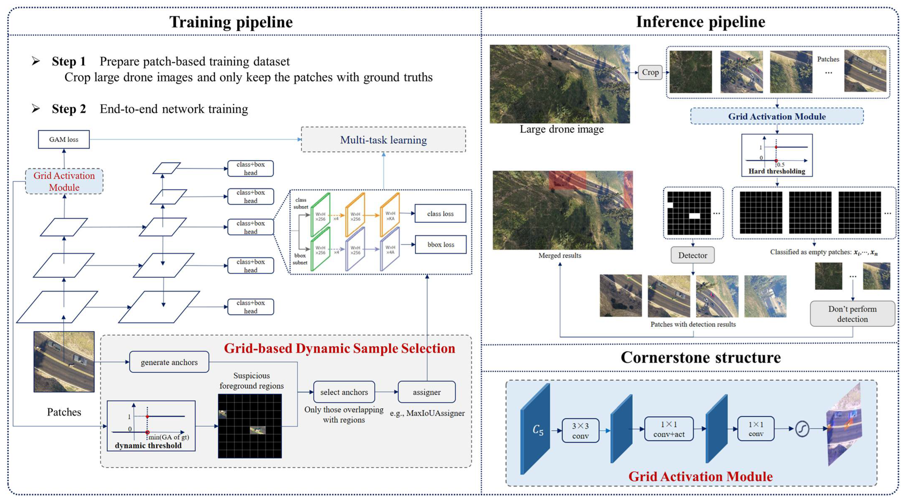
Hence, we introduce a novel approach, also in a tile-way, to accelerate inference speed and tackle background bias, thus enhancing detection accuracy. The overall workflow of the proposed detector in both training and inference stages is depicted in Figure 1. The GAM is the cornerstone of the proposed approach and is seamlessly integrated into both training and inference processes. Specifically, the GAM is built on a shared backbone with the detector to acquire grid activations, predicting whether each patch contains an object at the grid scale. During training, the GAM undergoes multi-task learning with the detection network. Additionally, GDSS, built upon the grid activations obtained by the GAM, dynamically filters positive samples and challenging negatives for learning. In the inference stage, by comparing grid activations with a hard threshold (e.g., 0.5), patches without any objects are rapidly filtered out, therefore avoiding subsequent detection processes, resulting in a significant speed improvement. Furthermore, we propose the GhostFPN, incorporating the Ghost module [24] and Depth-wise Separable Convolution [42] into Feature Pyramid Network (FPN), which reduces computation costs while preserving accuracy. Detailed explanations are provided in the following sections.

Figure 1.
GA-Net framework. (1) Training and inference pipeline: Training involves Grid-based Dynamic Sample Selection (GDSS) and multi-task learning towards end-to-end joint training. Inference involves cropping to patches and filtering out suspicious foreground patches to continue detection with grid activations surpassing a hard threshold. No operation on the backgrounds is performed, and finally the results are merged. (2) Network structure of the Grid Activation Module (GAM): It takes the feature layer from the backbone of the detection algorithm as its input, and produces corresponding grid activations using a simple classification head. 1 × 1 convolution is utilized to replace fully convolution layers to minimize computation costs.
3.2. Grid Activation Module
The GAM is a straightforward classification head, built on general feature extraction backbones, such as ResNet [43], ResNeXt [44], MobileNet V3 [45], and ShuffleNet V2 [46]. It rapidly defines the foreground regions at the grid scale, based on shared backbone features by calculating the probability of foreground presence in each grid. This module constitutes a crucial component of the proposed method in this paper. Specifically, during training, the GAM calculates grid activations, which assist GDSS to address the extreme foreground/background sample ratio. In inference, it facilitates the confidence estimation of foregroundness at the grid scale, speeding up detection by excluding background patches and performing detection solely on foreground patches. This module can be seamlessly integrated into various detector networks and trained end-to-end.
3.2.1. Network Architecture
By adding a classification head after a shared backbone of general detectors, we aim to obtain activations that represent the confidence of foregroundness. This is based on the observation that convolutional features associated with recognizable objects tend to exhibit significantly higher feature values when compared to other features in the feature map they belong to [18]. The architecture of the GAM is illustrated in Figure 2. We take ResNet50 as an example for the backbone. Given an image patch with the size of 512 × 512, we firstly divide it into smaller grids (e.g., 64 × 64). To extract features for the GAM, we utilize the feature maps from the last stage of ResNet50, denoted as . Obtained through the backbone, each pixel in corresponds to 32 pixels in the original patch. To create an activation map for 64-pixel grids, we employ a 3 × 3 stride convolutional layer. Now, the obtained feature map precisely corresponds to 64 pixels for each pixel, representing a grid in the original patch. This transforms the grid activation challenge into acquiring the activation for each pixel. We then adopt binary classification in order to attain the confidence of foreground presence. Typically, the general solution involves using a fully convolutional layer with an activation function on the feature map to generate the activation map. However, we learn from [15] to reduce computational costs by replacing fully convolution layers with 1 × 1 convolutional layers, thereby minimizing the additional computational overhead introduced by the GAM. The final activation map’s value at each pixel indicates the activation of its corresponding grid. Typically, we recommend selecting grid sizes that match the sizes of the objects of interest in the task. It is also advantageous to align the grid sizes with the feature maps from the backbone network, such as the final layer , to facilitate direct convolution for grid activations, as illustrated in the example above.

Figure 2.
Network architecture of the GAM.
The GAM features a straightforward structure that shares the backbone, reducing computational redundancy and facilitating the implementation of multi-task learning for end-to-end training and deployment. In contrast to directly classifying patches, where the network may struggle to define effective features, the GAM excels by subdividing complex problems into smaller-patches to grids, predicting at the scale suitable for classification, thus achieving higher accuracy.
3.2.2. Details in Training
As the GAM primarily serves for initial coarse searching followed by refined detection in our network, our priority lies in maximizing recall; that is, no potential objects should be missed. Suspicious ones are all intended for detailed scrutiny in the subsequent refined detection network. Therefore, when assigning learning labels to the GAM, we employ an Intersection-over-Foreground(IoF)-based approach in order to ensure the recall of all objects, regardless of the object scale compared to grid size.
We design the rule of label assignment in Figure 3. Instead of Intersection-over-Union, which calculates the intersection/union ratio, IoF calculates the intersection/foreground ratio. And here, grids or objects can both be the foreground. To illustrate, we take the example of a small object located in a grid as Patch x4 in Figure 3. Using IoU, the overlap should be the object area divided by the grid area, which is always small. But IoF calculates the overlap ratio as the object area divided by itself, which should be equal to 1. Also, for the case of large-scale objects in Patch x1, which might span across several grids, the IoF-based overlap would be the intersection area divided by the grid area, while IoU-based overlaps are too small to utilize the union area as the denominator.
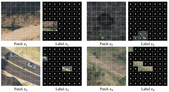
Figure 3.
Illustrations of the IoF-based label assignment for the GAM. The objects of Patch x1–x4 has decreased in scale successively. The diagram shows that using the IoF-based label assignment can effectively distinguish between foreground and background, facilitating the training of the classification head.
For the assignment, if a grid has an IoF-based overlap ratio with any ground-truth box higher than a pre-defined threshold, it is defined as positive; otherwise, the grid is negative. The formula is as follows:
Here, for each patch of size , we have a list of grids in size : . The binary label we assign is denoted by . denotes a set of ground-truth boxes of the objects in the image patch , and means the -th ground-truth box. is the function used to calculate the Intersection-over-Foreground overlap ratio. is the pre-defined threshold, and we set it as 0.2 in Figure 3.
It is crucial to emphasize that, whether dealing with single-class detection (e.g., cattle in our benchmark dataset) or multi-class detection as seen in public datasets, we disregard the categories of ground truth objects, focusing exclusively on the bbox position. We are learning the characteristics of the foreground. The class-independent GAM, when combined with the Grid-based Dynamic Sample Selection described later in Section 3, facilitates focused learning on (1) distinguishing between the foreground and background, especially discerning the foreground from potential false positives, and (2) distinguishing between different foreground categories.
In the training, we use a multi-task learning method to simultaneously optimize both the GAM and the detector. The overall loss is the sum of the GAM loss, classification loss, and bounding-box loss, defined as follows:
where and denote the classification loss and regression loss, respectively. Their definitions are identical to RetinaNet. is a parameter for balancing the losses. is the GAM loss defined as follows:
where is the number of grids, and is the activation of the grid defined above. is a classification loss, designed to address the issue of class imbalance by reducing the loss assigned to well-classified samples during training, which is defined as follows:
where parameters are set as , the same as in RetinaNet.
Multi-task learning not only achieves end-to-end training, but also benefits from the backpropagation of the GAM during joint optimization, which influences the backbone network to shift attention to important regions.
3.2.3. Details in Inference
In the inference stage, the pipeline is illustrated in the following pseudocode:
| Inference Pseudocode. |
| Input: Original image (I) Detected_Objects = [] for each cropped_patch in the original image: F = extract_feature_map(cropped_patch) # use backbone A = calculate_grid_activations(F) binary_map = (A > threshold T) if binary_map contains any non-zero values: detection_result = detector(F) # use neck and head Detected_Objects.append(detection_result) else: Detected_Objects.append(empty_result) Output: Detected_Objects (bounding box coordinates, class labels, confidence scores) |
As Figure 1 and the above pseudocode show, when provided with an original large image, we initially crop it into non-overlapping patches with a uniform size (e.g., 512 × 512). Then, we feed these patches into the backbone to extract feature maps F. Based on these feature maps, the GAM produces the grid activation map of the corresponding input patch. If the maximum value of the grid activations belonging to a patch surpasses a predefined threshold , the patch is defined as a foreground patch; otherwise, it is an empty patch. The refined detector can be any network, and in this paper, we use RetinaNet as the example. The detector, including the structure of Feature Pyramid Network and both classification and regression heads, will be only conducted on the foreground patches, skipping any operations for empty ones. Finally, we merge the outputs of the patches and obtain the results for the large image. To summarize, the grid activations play a crucial role in swiftly eliminating patches without objects during inference, allowing for refined detection that is solely on foreground patches. Through this rapid filtering, a large number of computations on unimportant regions can be avoided, resulting in a significant speed improvement.
3.3. Grid-Based Dynamic Sample Selection
GDSS is proposed here, based on the anchor-based network.
As depicted in Figure 4, the initial step is obtaining grid activations from the GAM. As we always have a batch of patches together to accelerate training, we set a batch-based dynamic threshold. Specifically, relying on the binary label we assign to the GAM, denoted by , the threshold is dynamically set as the minimum grid activation among all the grids containing objects in the batch. The formula is expressed as follows:

Figure 4.
The architecture of GDSS.
Assuming each batch has patches, denote the index of patch as . is the activation for the grid of the -th patch in the batch. is the binary label we assign to the grid of the -th patch in the batch, and when it is equal to 1, this indicates the presence of at least an object within the grid. We can imagine if a grid activation is larger than , the grid should contain either ground truth objects or challenging background instances, which are potential false positives.
These grids, considered as suspicious foreground regions, later undergo overlap calculations with the pre-defined anchors. Anchors that have no overlap with any selected grids will be discarded in subsequent label assignment. Only anchors overlapping with suspicious foreground regions are kept, and we then employ a general assigner on them to generate positive and negative samples. Consequently, the network focuses on learning from positive samples and challenging negatives, rather than struggle with numerous ‘easy background’ samples. This dynamic threshold avoids missing true values, as well as reduces the introduction of numerous negative samples from simple backgrounds, which results in a more condensed foreground coverage, enhancing learning efficiency and detection accuracy.
It is crucial to note that, in order to ensure training stability, in the initial iterations, we refrain from sample selection due to the uncertainty in the GAM initialization. This means that all anchors will undergo label assignment. During this phase, the GAM and the detector classification sub-network swiftly grasp simple background samples to learn. After just a few iterations, we activate the GDSS mechanism, focusing on distinguishing positive samples and complex backgrounds in the ongoing training.
To maintain consistency between training and inference, we also tried to employ a post-processing step with the same attempt to keep only the detections in suspicious foreground regions. This involves calculating the overlap between the detection results and predicted foreground grids, and preserve only the results with overlaps. Experimental results indicate that this attempt, compared to no post-processing, yields no discernible improvements. This essentially affirms that our GDSS method is effective enough in selecting patches that can train a robust network with a strong distinction between foreground and background. Therefore, we only apply the GDSS module during training, while the inference stage is still as outlined in Section 3.2.3, with no grid-scale after processing.
In summary, the integration of GDSS into basic one-stage models is explained above; by replacing the Region Proposal Network [9] with a straightforward foreground region search using the GAM, along with efficient sample selection occurring in training only, we enable the network to achieve a performance comparable to complex two-stage models in large scene scenarios and small objects. This is achieved without the need for extensive computational overhead, and also leverages the inherent advantage of rapid inference speed into one-stage models.
3.4. GhostFPN
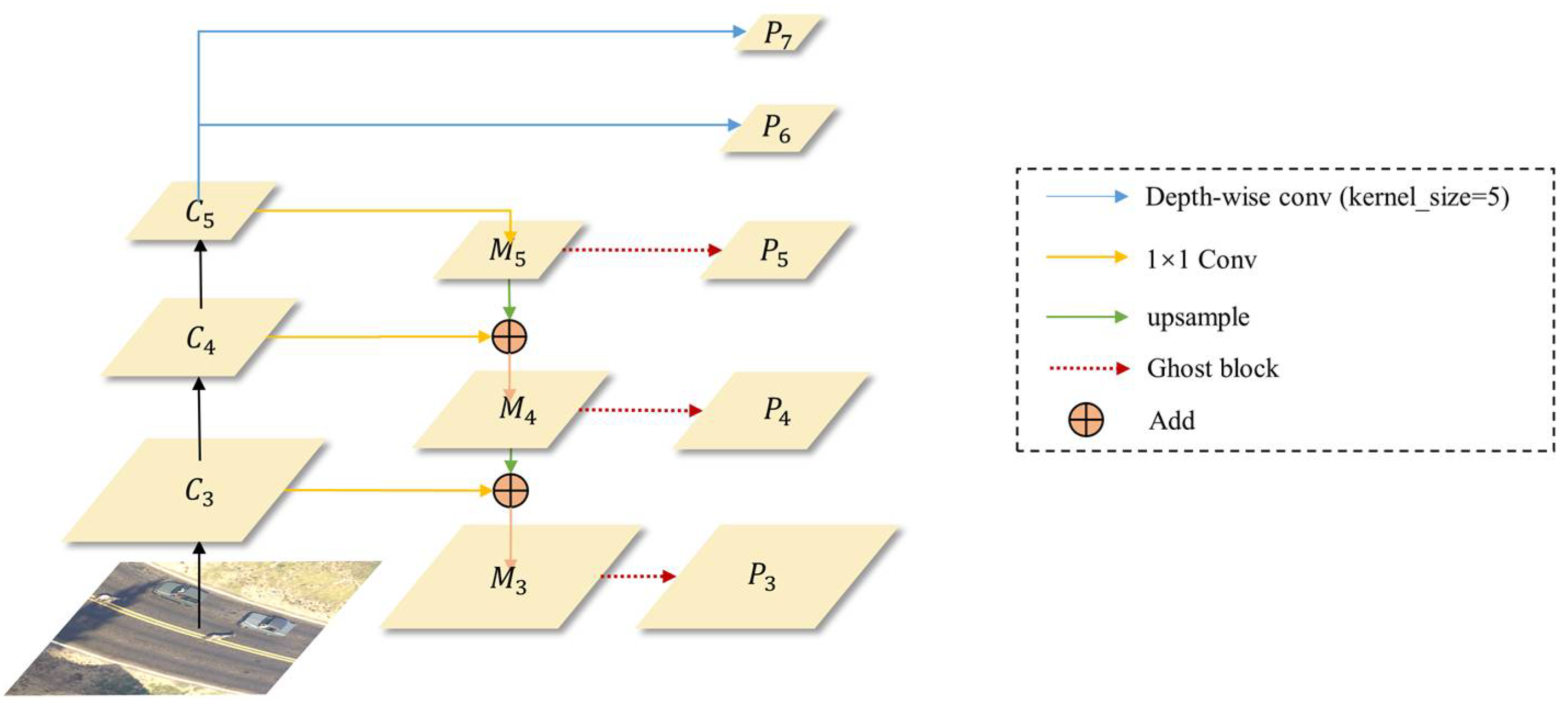
We present an improvement to the Feature Pyramid Network, termed GhostFPN, by incorporating the Ghost block and Depthwise Separable Convolution. This modification results in a reduction in computational costs while preserving performance. The structure of GhostFPN is illustrated in Figure 5. In contrast to the original FPN structure in RetinaNet, one of the improvements involves replacing the convolution operations used to generate multiple pyramid feature maps with the Ghost block from GhostNet. This substitution effectively reduces network computational and parameter overheads. Additionally, we replace the normal convolution layers responsible for generating P6 and P7 in RetinaNet with Depth-wise Separable Convolution featuring a 5 × 5 kernel. This alteration, made without increasing the parameters or the computational load, enlarges the receptive field, thus enhancing the contextual semantic information in higher-level feature maps.
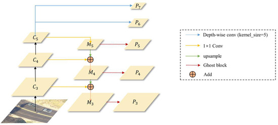
Figure 5.
The architecture of the GhostFPN.
To elaborate, the motivation behind the Ghost block is to mitigate the widespread redundancy in feature maps of mainstream CNN computations, thereby achieving network lightweighting through the utilization of this redundancy.
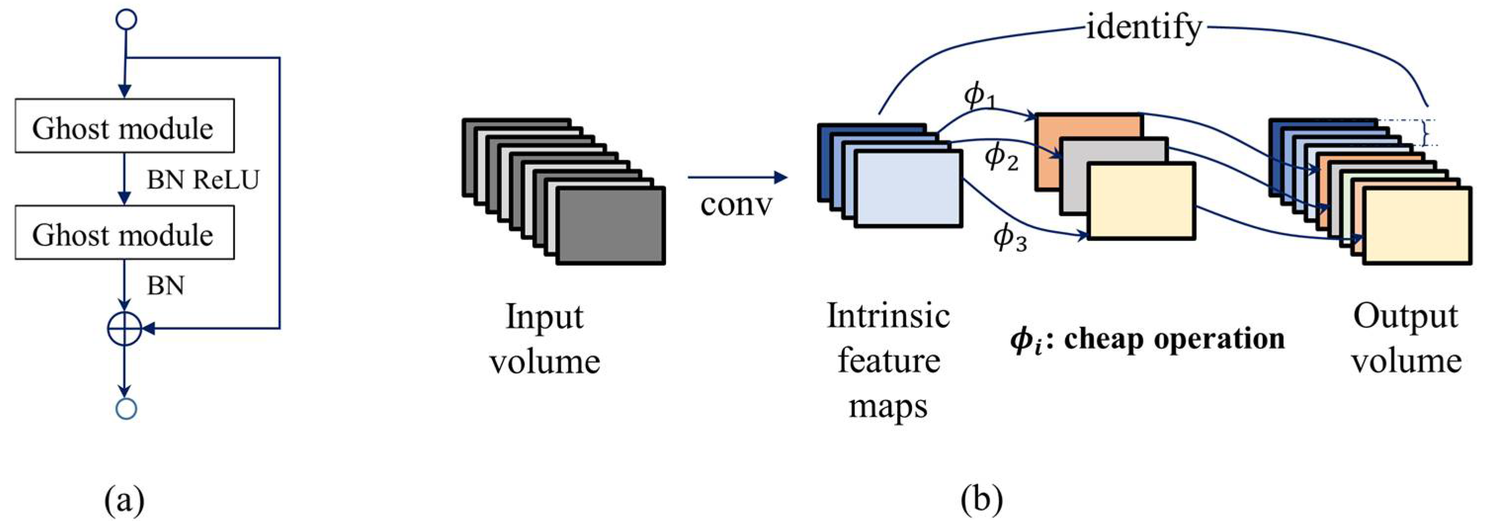
As illustrated in Figure 6a, the Ghost bottleneck is obtained by connecting two Ghost modules through residual connections. The first Ghost module functions as an expansion layer, augmenting the number of channels. Subsequently, the second Ghost module decreases the number of channels in order to align with the shortcut path. The shortcut is established between the inputs and outputs of these two Ghost modules.
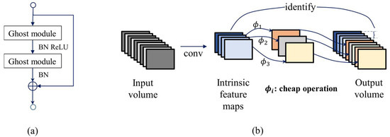
Figure 6.
Illustrations of Ghost block. (a) Structure of Ghost BottleNeck, the residual connection of two Ghost modules, and (b) Structure of Ghost module.
Figure 6b depicts the schematic diagram of the Ghost module, which consists of three steps: primary convolution, Ghost generation, and feature concatenation. In detail, intrinsic feature maps are first generated through primary convolutions. Step 2 is to apply linear cheap operations to produce redundant feature maps. Lastly, intrinsic feature maps and redundant feature maps are concatenated to obtain the output of the desired channels.
The cheap operation utilized in Step 2 is the Depth-wise Convolution. Depth-wise Convolution differs from traditional convolution in that it employs a separate convolution kernel for each input channel, rather than having each kernel simultaneously operate on all channels of the input volume. This helps reduce the number of parameters, thus improving computational efficiency.
However, this approach brings about two significant challenges. Firstly, the number of output channels can only be equal to the input layer’s, lacking flexibility in output. Secondly, this operation independently convolves each channel of the input layer, failing to effectively leverage feature information from different channels at the same spatial position. The second concern lies in the fact that this operation independently applies convolution to each channel of the input layer, failing to effectively utilize feature information from different channels at the same spatial position.
Therefore, Depth-wise Separable Convolution is proposed, extending the Depth-wise Convolution with Pointwise Convolution, which employs the 1 × 1 convolutional kernel to facilitate interactions between different channels, and can obtain the desired number of channels in the output. Consequently, Depth-wise Separable Convolution, akin to normal convolution, possesses strong representational capabilities and the flexibility of unrestricted input and output.
We conduct a comparison between the parameters and computational costs of the two approaches. Assuming a convolutional kernel size of , input channel number , and output channel number , the parameter count for a regular convolution is . In the case of Depth-wise Separable Convolution, the number of parameters is for the Depth-wise Convolution, and for the pointwise convolution. Therefore, the total number of parameters is . Since k is typically much smaller than , the reduction in parameters is substantial. For an input tensor of the same size, the computational cost is also significantly reduced. Even in cases where, as proposed in our GhostFPN, the kernel size of the Depth-wise Separable Convolution generating high-level semantic feature maps is set to 5, is still much smaller than (e.g., 256). According to the comparisons of the two convolutions discussed earlier, Depth-wise Separable Convolution with a larger receptive field still wins in reducing computational costs. This provides us with an effective solution to build higher-performing models in resource-constrained environments.
4. Experimental Results and Analysis
To assess the efficiency and precision of the GA-Net framework designed for drone images in this study, we first further extended the data collection on the synthetic GTAV-Cattle dataset [26], and created a new dataset, GTAV-Cattle-v2, serving as our benchmark dataset. Subsequently, we performed experiments on the benchmark dataset to compare the performance of GA-Net with its baseline, as well as with state-of-the-art models. The efficacy of the proposed method was further validated on publicly available datasets, covering diverse scenes, including maritime, traffic, and urban scenarios. An extensive ablation study was also conducted to measure the contributions of the GAM, the GDSS, and the GhostFPN.
4.1. Datasets and Evaluation Metrics
As Figure 7 shows, in traditional cases, datasets for evaluating object detection models exclude background images from validation or test sets. However, in real surveillance scenarios, numerous images are ‘empty’ without any objects. They would not tell whether the scene contains objects before inspection. Therefore, to facilitate low-latency and accurate detection research in real-world applications, we introduce a modified variant of DGTA-Cattle, which we refer to as DGTA-Cattle-v2. The key modification is the inclusion of numerous images without targets in the validation and test sets by leveraging the convenience of generating images using GTA, which reflects the common occurrence of no-object scenes in real surveillance scenarios.
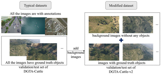
Figure 7.
An illustration of how we modified DGTA-Cattle dataset to DGTA-Cattle-v2.
As Table 1 shows, besides DGTA-Cattle-v2, we also select three public datasets encompassing various scenes, including maritime, traffic, and urban scenarios. VisDrone-Det [47] and SeaDronesSee [48] are collections of UAV recordings, while DOTA [49] primarily comprises satellite-recorded images. Specifically, VisDrone-vehicle and DOTA-vehicle are variants focusing solely on vehicle-like objects, such as cars, vans, trucks, and buses. This intentional selection aims to present more background pixels to aid in evaluating our proposed model.

Table 1.
Datasets used in the study for evaluation and detailed comparisons.
- DGTA-Cattle-v2
DGTA-Cattle is chosen for its flexible data collection approach within the Grand Theft Auto V (GTAV) video game environment. This dataset is uniquely created by utilizing GTAV as a simulation engine and adapting it to UAV settings. It is a large-scale, high-resolution (4K) synthetic object detection dataset, where various cattle models are placed in diverse scenarios to interact with realistic graphics and physics simulations in a vast world. The dataset allows for adjustments in camera positions, rotation, environment manipulation, object spawning, and the rendered resolution, according to specific requirements, with the automatic acquisition of bounding box annotations.
We leveraged the flexibility of GTAV for acquiring data. To validate our proposed model, the dataset was meticulously designed to encompass diverse scenarios, incorporating variations in background, object distribution density, shooting altitude, visibility range, tilt angles, light conditions, and shadows. The dataset provides precise 2D bounding boxes for the unique target category ‘cattle’. Additionally, we automated the collection of numerous no-object background images, adding them to the validation and test sets. The training set, aimed at enhancing the effectiveness of data training and information density, deliberately excludes such purely background images without objects. In summary, our training set comprises 4000 images, the validation set includes 1000 images, and the test set consists of 1139 images. Each image maintains a uniform size of 3840 × 2160 pixels, with the majority of objects being of a small scale. The scale of foreground areas varies with flying altitudes and observing viewpoints. In our subsequent experiments, the validation set is utilized for selection of the best performance model, while the test set is employed for evaluating the performance metrics. Figure 8 provides a visual representation of the size distribution of object-bounding boxes in the dataset, where the horizontal and vertical coordinates indicate the width and height of the targets, respectively. It can be seen that the size distribution is predominantly concentrated in the lower-left corner, signifying that the majority of objects in the dataset are small.
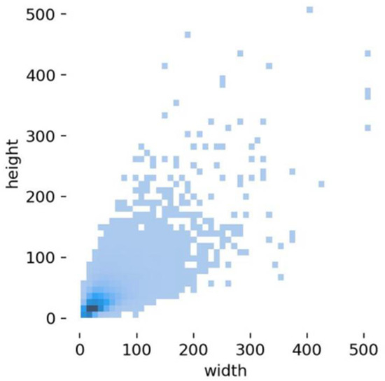
Figure 8.
Size distribution of DGTA-Cattle-v2 dataset.
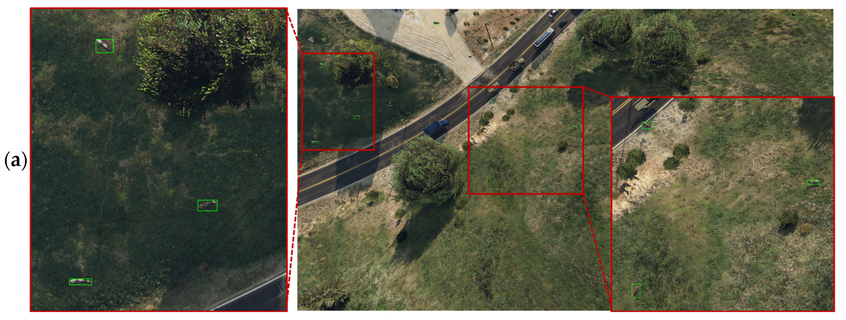
To provide a more vivid depiction of the DGTA-Cattle-v2 dataset, Figure 9 showcases a set of images alongside their corresponding annotations. For enhanced clarity, specific areas are zoomed in to illustrate the annotations of objects in detail. The objects are proportionally small when compared to the overall field of view, and the scenes are complex. In such scenarios, even human visual inspections for target search and localization can be time consuming.

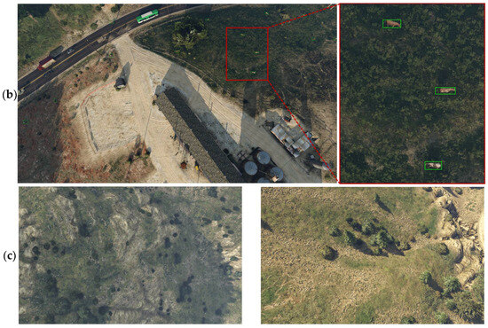
Figure 9.
Examples of images in the DGTA-Cattle-v2 dataset. (a,b) Images with annotated bounding boxes for cattle, marked by green rectangles. To provide a clearer view of the appearance of small targets, a zoomed-in version is highlighted with a red box; (c) Pure background images without any objects.
- VisDrone-vehicle
For our experiments, we use the detection task (VisDrone-DET). The dataset comprises a total of 10,209 images, with 6471 images allocated for training, 548 for validation, and 3190 for testing. The image resolutions range from 960 × 540 to 2000 × 1500. The dataset is specifically designed for traffic surveillance applications in urban areas.
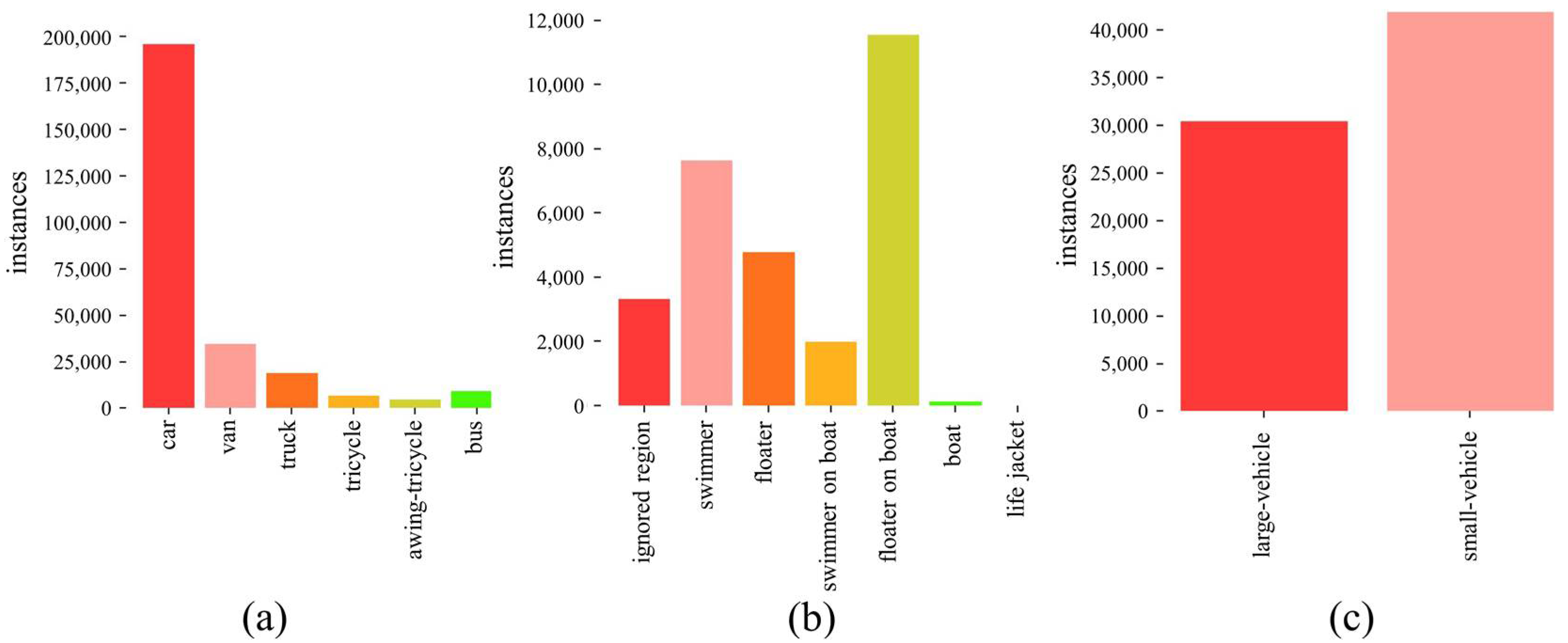
Captured by drone-mounted cameras in 14 different cities, the dataset has 10 manually annotated categories, including pedestrian, people, bicycle, car, van, truck, tricycle, awning-tricycle, bus, and motor. For our experiment, we only keep the annotations of six vehicle-like categories, as illustrated in Figure 10a. Other annotations are discarded, but images without objects of interest are retained, allowing the model to autonomously determine if there are any objects of interest in an image. They act as pure background, akin to those in our GTAV-Cattle-v2 dataset. This gives the dataset a higher background ratio, increasing background complexity, while maintaining class imbalance and addressing significant scale change issues. As the test set is not public for this dataset, we use the validation set for the evaluation, which is common practice [21,22].

Figure 10.
Object categories and counts: (a) VisDrone-vehicle; (b) SeaDronesSee; (c) DOTA-vehicle.
We visualize sample images of VisDrone-vehicle dataset in Figure 11, with annotated ground truths for different categories delineated by rectangles of varying colors.

Figure 11.
Annotation examples of VisDrone-vehicle dataset, with purple boxes annotating ‘car’, orange boxes annotating ‘bus’ and red boxes framing out ‘ignored regions’.
- SeaDronesSee
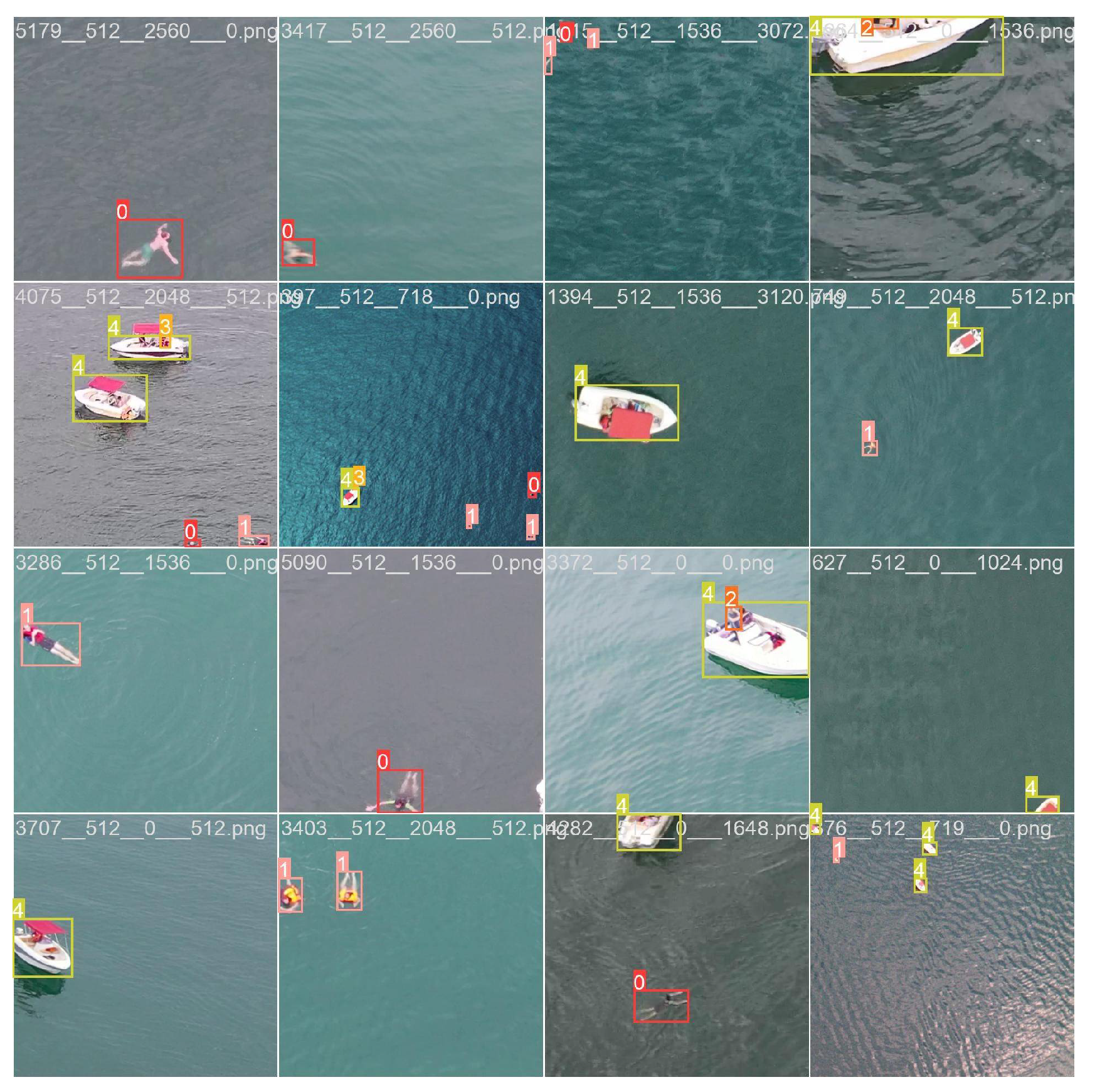
SeaDronesSee is designed for maritime environments, which can aid in the search and rescue application. The training set includes 2975 images with 21,272 annotations. The resolutions of the images range from 931 × 1227 pixels to 5456 × 3632 pixels. The reported accuracy is assessed on the validation set, which consists of 859 images. See Figure 10b for the object categories and distributions over the categories. We visualize sample patches of the SeaDronesSee dataset in Figure 12 in order to show the annotations.

Figure 12.
Annotation examples of the SeaDronesSee dataset. Numbers 0-4 on the upper-left of the boxes correspond to ‘swimmer’, ‘floater’, ‘swimmer on boat’, ‘floater on boat’ and ‘boat’, respectively.
- DOTA-vehicle
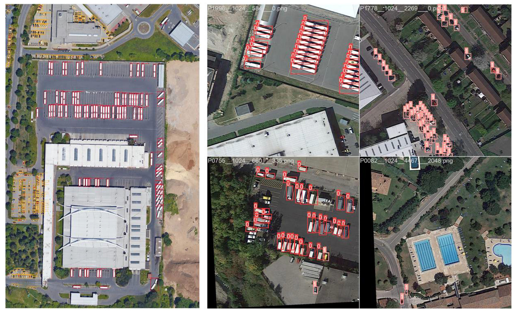
DOTA is a comprehensive benchmark dataset, designed for object detection in aerial images, offering large-scale and high-resolution imagery. The dataset exhibits a wide range of image resolutions, spanning from 475 × 547 pixels to 29,200 × 27,616 pixels. Given that the test set is not publicly available, we utilize the validation set, consisting of 458 images. Similar to our approach with other datasets, we focus exclusively on vehicles, retaining vehicle annotations, while treating other objects as background instances. The background images are retained, allowing the model to autonomously determine the presence of objects of interest. Refer to Figure 10c for the kept object categories and object counts. We visualize some annotations of the DOTA-vehicle dataset in Figure 13 to emphasize the annotations.
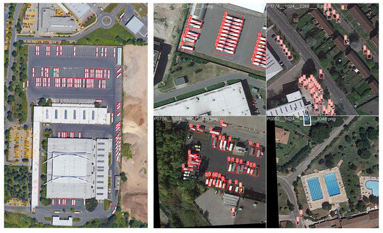
Figure 13.
Annotation examples of the DOTA-vehicle dataset. In the entire image (left), red boxes annotate ‘large vehicle’ and orange boxes annotate ‘small vehicle’. In the patches (right), 0 and 1 on the upper-left of the boxes correspond to ‘large vehicle’ and ‘small vehicle’ respectively.
- Metrics
In our research, we adhere to the standard evaluation protocol established by MS COCO, where the overall performance, in terms of the mean average precision (mAP), is measured by averaging over different categories and multiple intersection-over-union (IoU) thresholds, ranging from 0.5 to 0.95, with an interval of 0.05. The model complexity is evaluated in terms of Giga floating-point operations (GFLOPs) and the total parameter count. The inference speed is quantified in frames per second (FPS).
4.2. Implementation Details
GA-Net is implemented using PyTorch. The experiments are conducted on a single NVIDIA GeForce RTX 2080 Ti for each task. RetinaNet is chosen as the baseline detector, and six other well-established and state-of-the-art models are used as comparison detectors. ResNet50 is employed as the feature extraction backbone for all the models, except for YOLOv8, which utilizes its originally designed backbone. Networks are trained using the AdamW optimizer with a cosine annealing learning strategy, incorporating a linear warm up. The initial learning rate is set to 1 × 10⁻⁴, and the weight decay is set to 0.01. All models undergo training for 24 epochs.
It is important to note that the experimental settings vary for different datasets. For DGTA-Cattle-v2, the training set is used for learning, the validation set is employed for the model selection, and the test set is utilized for testing. As for VisDrone-vehicle, SeaDronesSee, and DOTA-vehicle, the training set is used for learning, and the validation set is for testing. DGTA-Cattle-v2 and SeaDronesSee are cropped into 512 × 512 patches, VisDrone-vehicle is cropped into 256 × 256 patches, and DOTA-vehicle is cropped into 1024 × 1024 patches. During training, an overlap of 0.2 is introduced between patches, while, during inference, no overlap is applied. For all experiments, flip augmentation is applied with a probability of 0.5. During training, no additional data augmentation is used, except for random flipping, including the modified YOLOv8.
4.3. Comparative Experimental Results and Analysis
We conducted experiments on DGTA-Cattle-v2, VisDrone-vehicle, SeaDronesSee, and DOTA-vehicle datasets, comparing our method to state-of-the-art object detectors.
4.3.1. DGTA-Cattle-v2
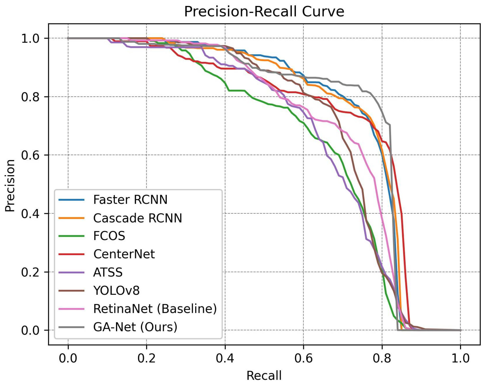
On the DGTA-Cattle-v2 dataset, in addition to our baseline detector RetinaNet [11], we conducted a comprehensive comparison with six recent or popular methods, including Faster RCNN [9], Cascade RCNN [50], FCOS [51], CenterNet [52], ATSS [33], and a modified variant of YOLOv8, where we use the same data augmentation as all the other experiments. The experimental results are presented in Table 2 and Figure 14. In Table 2, we categorize these models into one-stage and two-stage approaches. It is observed that two-stage models outperform one-stage counterparts in accuracy; however, this advantage comes at a significant cost in terms of speed. Our GA-Net, built upon the baseline RetinaNet, achieves a remarkable 4.2% improvement in accuracy, surpassing all one-stage models, and approaching the accuracy level of two-stage models. Furthermore, GA-Net further leverages the inherent speed advantage of one-stage models, surpassing the two-stage model by more than twofold, and demonstrating a 70% increase in speed when compared to the baseline. This outcome convincingly demonstrates the superior performance of our technique, achieving an advantageous scenario both in terms of detection accuracy and speed.

Table 2.
Comparisons of GA-Net with baseline and state-of-the-art on DGTA-Cattle-v2 dataset.

Figure 14.
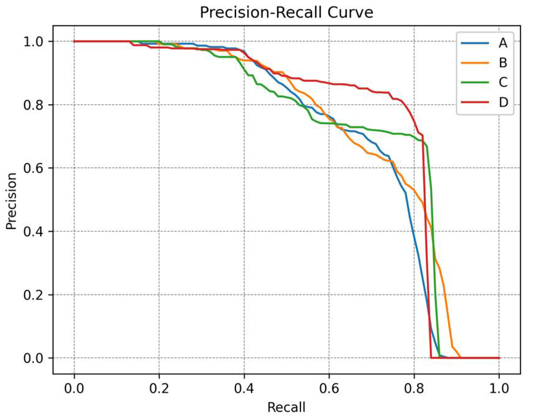
P-R curves of different algorithms.
Figure 14 illustrates the precision–recall curves of our proposed model, the baseline model, and state-of-the-art algorithms when the IoU threshold is set to 0.5. The P–R curves provide a comprehensive assessment of both precision and recall, with the area under the curve (AUC) representing the overall performance. Generally, a better detector is visually represented by a larger AUC. In this context, our proposed model significantly improves the detection accuracy when compared to the baseline RetinaNet, reaching a level comparable to two-stage models.
It is essential to highlight that, to investigate the effectiveness and significance of the proposed enhancements, our GA-Net is implemented without incorporating any additional tricks. Techniques such as data augmentation, training strategies, and even multi-scale testing could be further employed to achieve an even superior performance.
To offer a more vivid and direct comparison among these models, in Figure 15, we have visualized the prediction results of the proposed model, the baseline, and Cascade RCNN, which stands out among the state-of-the-art detectors on the dataset. When taking a close look at the original drone image examples shown in Figure 15, particularly the areas enclosed by dashed boxes, our GA-Net exhibits the effective elimination of false positives as predicted by the baseline, achieving more precise detection results when compared to Cascade RCNN.
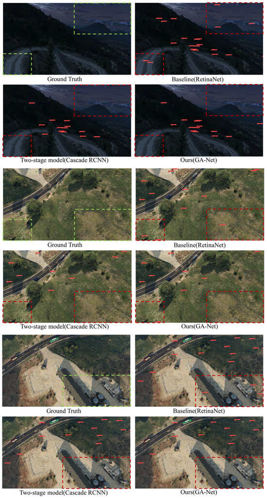
Figure 15.
Visualizations are presented in comparison with the top-performing Cascade RCNN and the baseline. Due to the large overview of the original images, we have highlighted specific regions in three sets of images by dashed boxes for better visibility. Notably, the baseline exhibits false detections, while both our GA-Net and Cascade RCNN can effectively avoid such false positives.
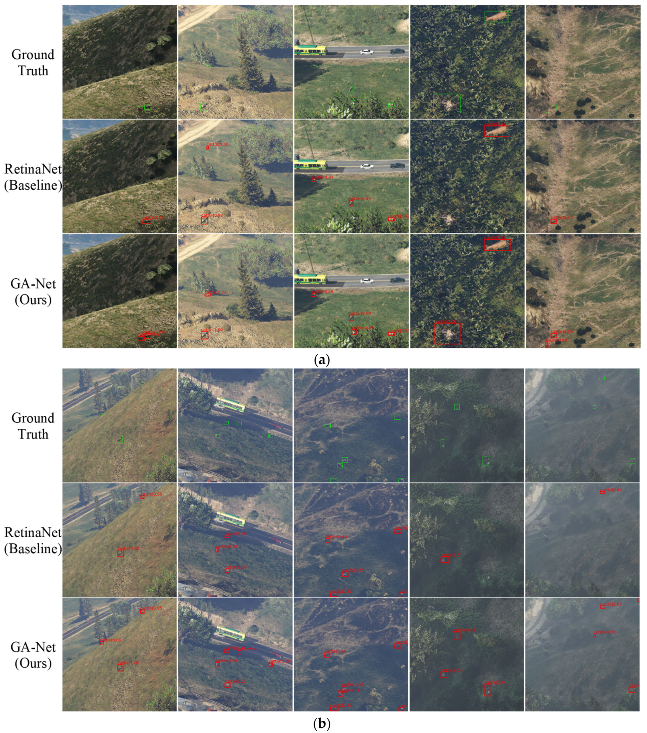
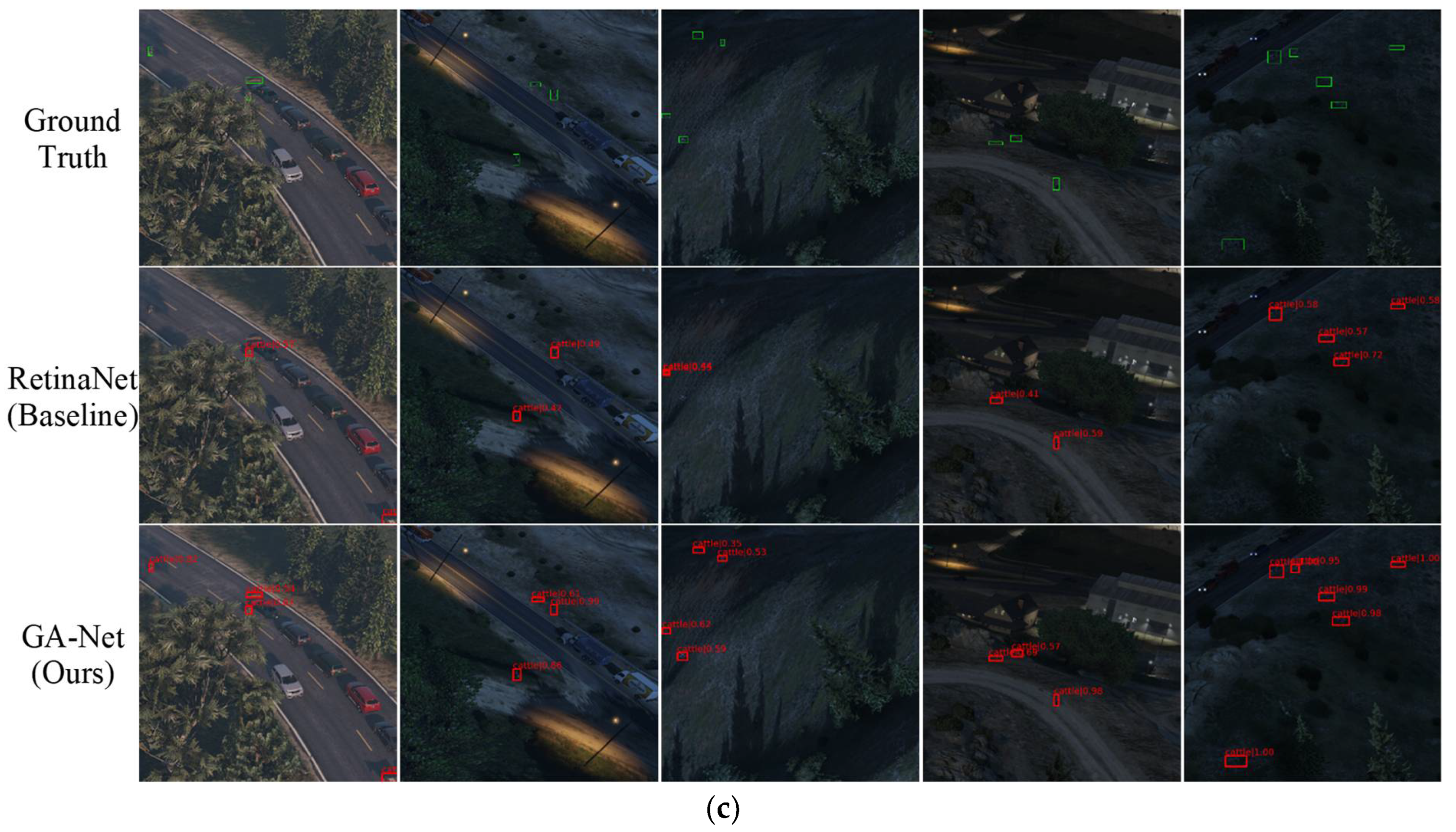
To emphasize the distinctions, as shown in Figure 16, we have visualized the detection results with the same confidence threshold of 0.35 on patches, which act as magnifiers for the global images, showcasing the superior detection accuracy, compared to the baseline. We have chosen three sets of scenarios, namely daylight, foggy, and dark, to highlight the adaptability of our model to different situations. In the first rows, ground truth is annotated with green boxes, while the second and third rows visualize the detection results of the baseline and the GA-Net with red boxes, accompanied by the predicted categories and confidence scores. It is evident that our approach has made significant improvements in detecting small and challenging targets, even including those under occlusion and camouflage.
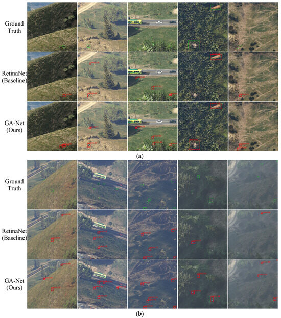
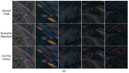
Figure 16.
Visual representations of patch results in varied shooting environments: (a) Daylight, (b) Foggy, and (c) Dark.
In summary, our model not only excels in eliminating false positives, but also enhances the detection capability of challenging targets. Furthermore, it significantly boosts inference speed, making it exceptionally valuable for UAV detection, especially in scenarios demanding low latency.
4.3.2. VisDrone-Vehicle
In the case of the VisDrone-vehicle dataset, our method is compared to the baseline model RetinaNet and the two-stage model Faster RCNN. As illustrated in Table 3, our approach, without bells and whistles, improves the accuracy of the base detector by 2.4%, while reducing GFLOPs and Params, resulting in a 27% speed boost. The accuracy is elevated close to that of two-stage models, yet the model complexity and computational load metrics remain significantly lower than those of two-stage models. The less pronounced speed improvement compared to GTAV-Cattle-v2 is attributed to a lower number of pure background cropped patches in this dataset. Generally, in scenes where targets are more locally distributed and the background proportion is higher, GA-Net exhibits a more noticeable improvement in inference speed.

Table 3.
Comparison of GA-Net against two-stage model Faster RCNN and baseline detector RetinaNet on VisDrone-vehicle dataset. ‘FPS’ is obtained by averaging inference speed of the whole validation set.
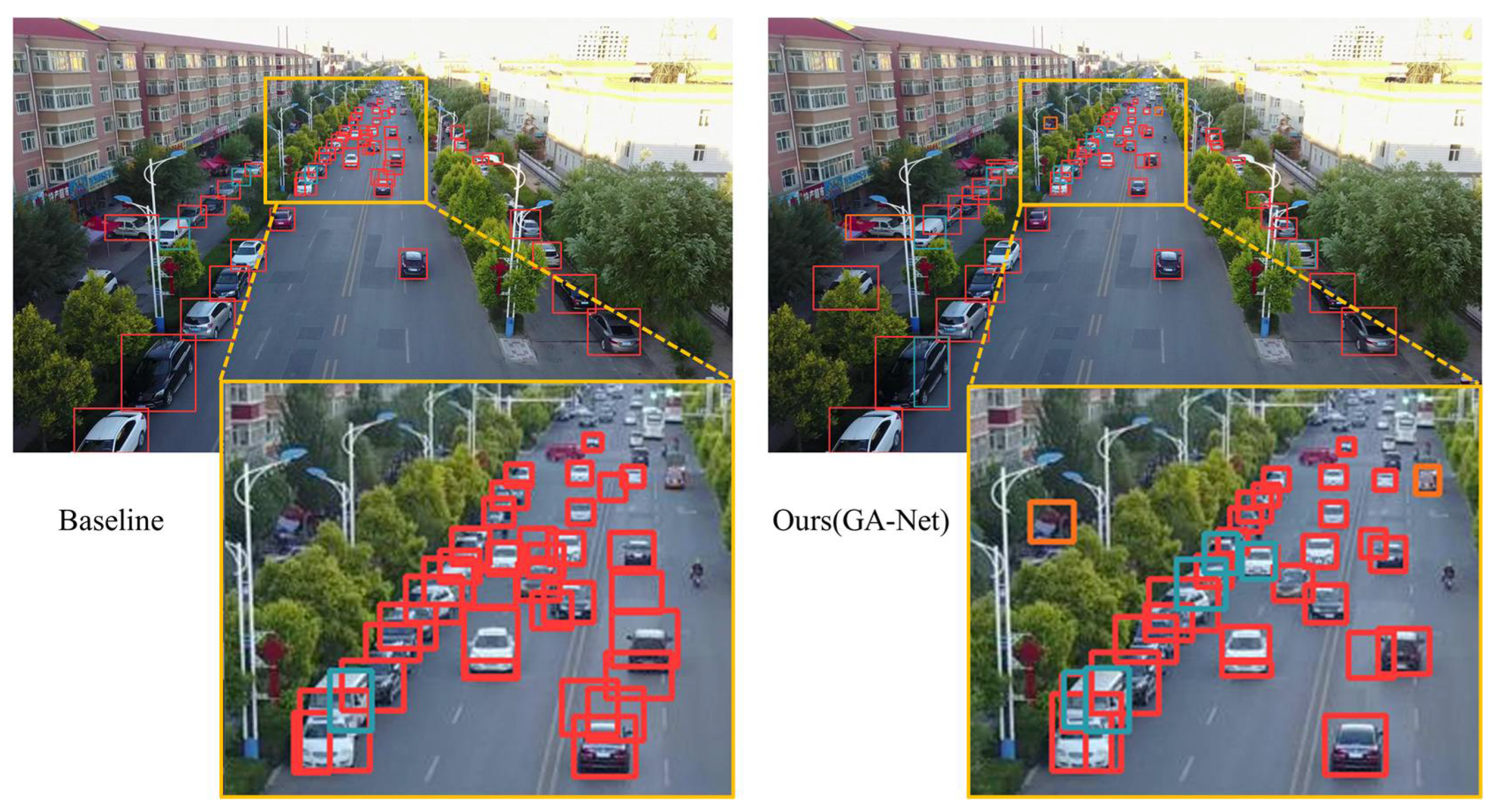
The detection results of the base detector RetinaNet and our proposed GA-Net are visualized with the same confidence threshold of 0.35, as shown in Figure 17. The orange box shows a zoomed-in version of a local region full of small vehicles. A comparative analysis of the two results clearly demonstrates the superior performance of our proposed GA-Net in detecting small targets.

Figure 17.
Visualizations are presented in comparison with the top-performing Cascade RCNN and the baseline. Due to the large overview of the original images, we have highlighted specific regions in three sets of images by dashed boxes for better visibility. Notably, the baseline exhibits false detections, while both our GA-Net and Cascade RCNN can effectively avoid such false positives.
4.3.3. SeaDronesSee
For the SeaDronesSee dataset, we conducted similar comparisons. As demonstrated in Table 4, our approach improves the accuracy of the base detector by 0.6%, while reducing GFLOPs and parameters, resulting in a 64% increase in speed. The SeaDronesSee dataset is characterized by a uniform background. Through the use of the GAM, we can swiftly filter out background scenes, thereby enhancing inference speed. However, GDSS does not yield a significant improvement in accuracy when compared to the baseline model. This is because the Focal Loss applied in RetinaNet is already effective in autonomously suppressing the learning weights of these simple background samples, thus achieving a similar effect to Grid-based Dynamic Sample Selection. This experiment demonstrates that our proposed method is more effective in scenarios with complex backgrounds, as seen in DGTA-Cattle-v2. Nevertheless, for scenarios with simple backgrounds, our proposed method remains effective in improving speed.

Table 4.
Comparison of GA-Net against two-stage model Faster RCNN and baseline detector RetinaNet on SeaDronesSee dataset. ‘FPS’ is obtained by averaging inference speed of the whole validation set.
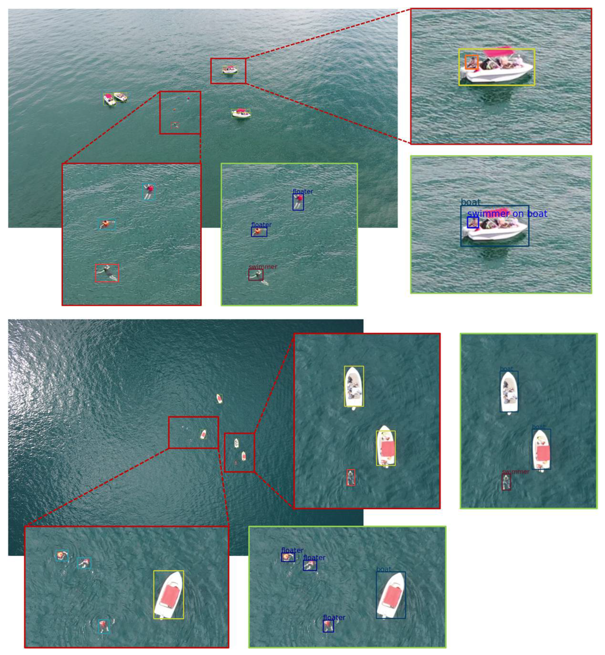
As the accuracy improvement is not substantial, and, in most cases, the visualizations of the baseline model and GA-Net are similar, we specifically zoom in to closely examine the matched detections of our GA-Net with ground truth objects, as shown in Figure 18.
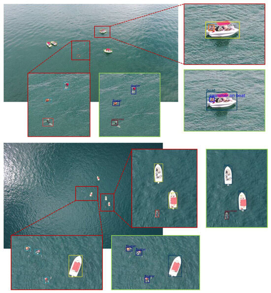
Figure 18.
Detection results are shown in a zoomed version by red frames, while the corresponding ground truth objects, along with their categories, are outlined in adjacent green frames.
4.3.4. DOTA-Vehicle
For the DOTA-vehicle dataset, as illustrated in Table 5, our approach improves the accuracy of the base detector by 3.8%, achieves a 33% increase in speed, and simultaneously reduced GFLOPs and Params.

Table 5.
Comparison of GA-Net against two-stage model Faster RCNN and baseline detector RetinaNet on DOTA-vehicle dataset. ‘FPS’ is obtained by averaging inference speed of the whole validation set.
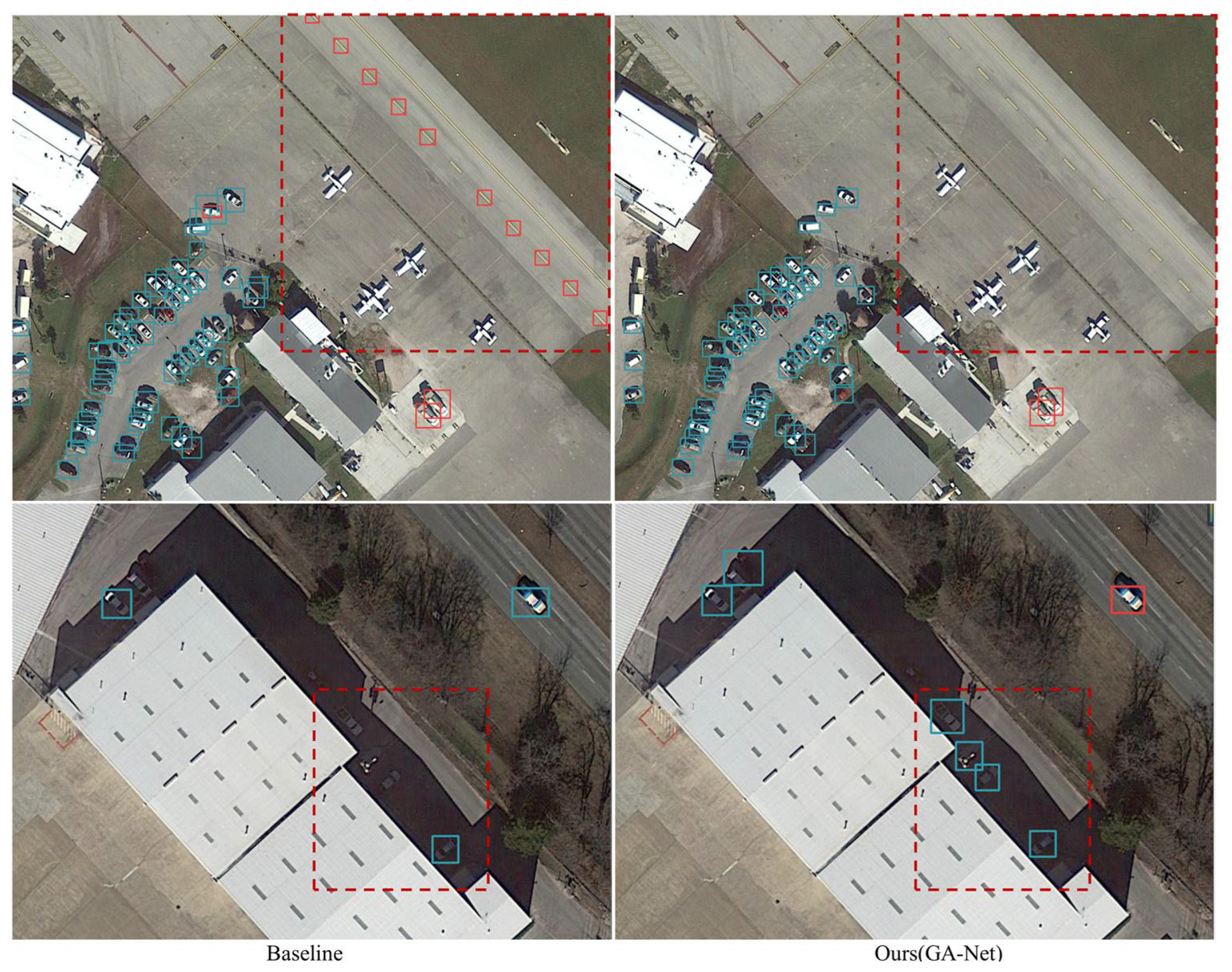
In the DOTA-vehicle dataset, as we only retain annotations for vehicles in our learning process, images without ‘background’ vehicles are also preserved. This leads to the inclusion of numerous ground instances prone to confusion, as depicted in the first row of Figure 19. In this row, the baseline and GA-Net detection results are highlighted by red rectangles. The base detector misidentifies airport runway lines as large vehicles, while our proposed model successfully removes such false positives. As shown in the second row, the red frames in the comparative results highlight our model’s accurate detection of challenging vehicle instances. This demonstrates the adaptability of the proposed GA-Net to complex scenarios.
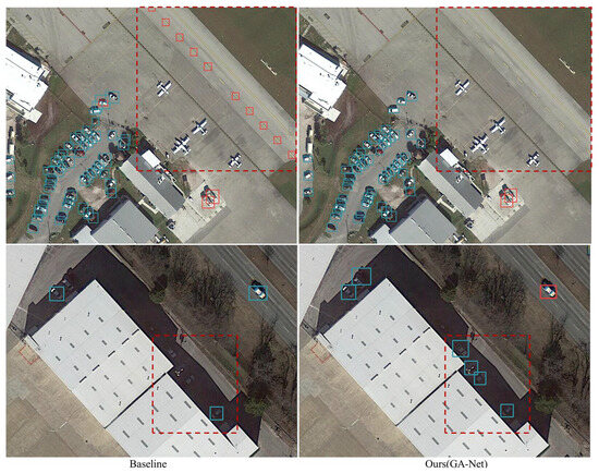
Figure 19.
Visualizations of detections using the baseline model and GA-Net. The first column displays the detections of the baseline model; the second shows predictions from GA-Net.
4.4. Ablation Study
To further validate the effectiveness of our proposed model, we conducted an extensive ablation study on the DGTA-Cattle-v2 dataset.
4.4.1. Comparison with the Baseline Model
We carried out a comprehensive evaluation on the DGTA-Cattle-v2 test set to accurately assess the performance of each proposed component on the baseline RetinaNet. These enhancements include the GAM, the GDSS, and the GhostFPN. Our evaluation takes into account both detection accuracy and efficiency, utilizing a diverse set of metrics: mAP, AP50, GFLOPs, Params, and FPS. The experimental results are presented in Table 6 and Figure 20.

Table 6.
Ablation study results on the DGTA-Cattle-v2 dataset.
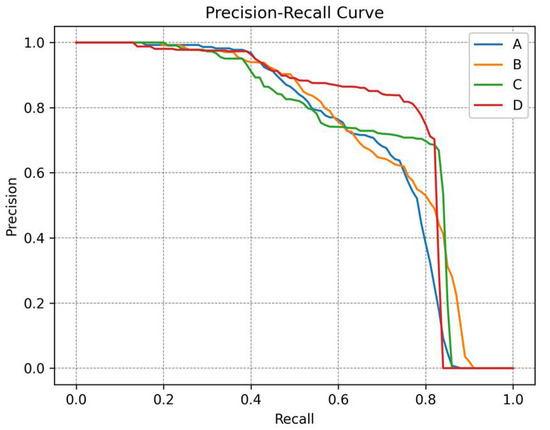
Figure 20.
P–R curves of different configurations: (A) Baseline RetinaNet, (B) Baseline with the GhostFPN replacing the FPN, (C) Baseline with the GAM and the GhostFPN replacing the FPN, and (D) the proposed GA-Net.
- The modification of FPN to GhostFPN leads to improved detection metrics. This change reduces params by 16.68%, as well as decreased GFLOPs from 52.28 to 49.57, which showcases the efficiency in lightweighting the model. We also note improvements in mAP and AP50 by 1.6% and 2.1%, respectively. Additionally, the FPS slightly increases by 1.42%.
- The incorporation of the GAM slightly increases memory usage and GFLOPs. However, when coupled with GhostFPN, these metrics remain lower than those of the base detector. Without GDSS in training, just by removing the background patches predicted by the GAM, the accuracy can still be slightly improved by 0.7% in mAP and 0.3% in AP50 based on the modification of FPN to GhostFPN. Notably, the speed receives a boost of 56.97%, attributed to the coarse filtering before the refined detection process.
- The use of the GDSS strategy in training directs the model’s attention towards foreground areas, contributing to the additional 1.9% increase in performance, building upon all the other proposed modifications. Furthermore, under the mutual influence of multi-task learning, the GAM can filter foreground patches more accurately, leading to a further improvement in inference speed, surpassing the base detector by 71%.
4.4.2. Effect of the GAM on Two-Stage Models
For two-stage detectors, as the Region Proposal Network (RPN) inherently addresses the issue of sample imbalance, there is no need for sample selection. Therefore, we only apply the GAM to assist inference, and do not incorporate GDSS during training. As shown in Table 7 and Table 8, our GAM boosts the detection speeds of Faster R-CNN by 23.0% on DOTA-vehicle dataset, and 41.0% on VisDrone-vehicle dataset, respectively, meanwhile improving the accuracy to an extent.

Table 7.
Comparisons of incorporating the GAM or not on Faster RCNN on the DOTA-vehicle dataset.

Table 8.
Comparisons of incorporating the GAM or not on Faster RCNN on the VisDrone-vehicle dataset.
Overall, the ablation experiments provide valuable insights into the effectiveness and significance of each enhancement, thus underscoring the potential of the proposed improvements to elevate accuracy, while concurrently boosting the inference speed.
5. Discussions and Conclusions
To address the challenges inherent to UAV platforms, such as the detection of small objects, background bias, and the need for low-latency processing, we propose GA-Net, an accurate and efficient detector for UAV-based images based on grid activations. The core of our approach is the GAM, a pivotal component that efficiently searches foreground regions at the grid scale with minimal computations. By leveraging grid activations, we avoid redundant detections on background patches to boost inference speed and utilize GDSS to shift the focus of learning towards challenging key areas, mitigating bias towards simple backgrounds. Moreover, our GhostFPN module not only reduces computational costs, but also contributes to increased accuracy. To assess the effectiveness and versatility of our proposed detector, we first modified a synthetic dataset, DGTA-Cattle, by introducing background images to simulate real surveillance scenes. Subsequently, we validated the efficacy of our methodology through comparative experiments with state-of-the-art methods and an ablation study on the new DGTA-Cattle-v2 dataset, along with three datasets from various domains (VisDrone, SeaDronesSee, DOTA). Although in this paper, our GA-Net only applies the enhancements on the baseline RetinaNet, there is a broader applicability. Any one-stage models can benefit from GDSS to address background bias, while the GAM can be seamlessly adopted by both one-stage and two-stage models to accelerate inference, with end-to-end joint training.
Moving forward, our future research will focus on seamlessly integrating this software algorithm into UAV hardware platforms. This includes exploring robust deployment strategies to ensure real-time performances on drone images, as well as adaptability to different operating environments. By transitioning from software validation to hardware implementation, we aim to bridge the gap between algorithmic innovation and practical deployment, ultimately contributing to effective and low-latency UAV detection systems. Furthermore, in addition to the implications for UAV applications, we hope our proposed method can also potentially benefit various computer vision tasks, including autonomous driving, robotics, and surveillance systems, where real-time and efficient object detection is crucial.
Author Contributions
Conceptualization, R.Z. and B.L.; methodology, R.Z.; software, R.Z.; validation, R.Z.; formal analysis, R.Z.; investigation, R.Z. and B.L.; resources, X.S. and J.L.; data curation, R.Z.; writing—original draft preparation, R.Z.; writing—review and editing, X.S. and J.L.; visualization, R.Z.; supervision, B.L.; project administration, B.L. and J.L.; funding acquisition, J.L. All authors have read and agreed to the published version of the manuscript.
Funding
This paper was supported by National Natural Science Foundation of China (No. 61801332 and No. 62371348).
Data Availability Statement
The datasets analyzed in this study are publicly available. Specifically, the DGTA-Cattle, VisDrone, SeaDronesSee, and DOTA datasets can be accessed through their respective official channels. Additionally, for convenience, we have provided download links for our modified datasets on GitHub repository: https://github.com/zhgruiyi/GA-Net/blob/main/dataset.md (accessed on 8 January 2024).
Conflicts of Interest
The authors declare no conflicts of interest.
References
- Hayat, S.; Yanmaz, E.; Muzaffar, R. Survey on Unmanned Aerial Vehicle Networks for Civil Applications: A Communications Viewpoint. IEEE Commun. Surv. Tutor. 2016, 18, 2624–2661. [Google Scholar] [CrossRef]
- Nex, F.; Armenakis, C.; Cramer, M.; Cucci, D.A.; Gerke, M.; Honkavaara, E.; Kukko, A.; Persello, C.; Skaloud, J. UAV in the Advent of the Twenties: Where We Stand and What Is Next. ISPRS J. Photogramm. Remote Sens. 2022, 184, 215–242. [Google Scholar] [CrossRef]
- Byun, S.; Shin, I.-K.; Moon, J.; Kang, J.; Choi, S.-I. Road Traffic Monitoring from UAV Images Using Deep Learning Networks. Remote Sens. 2021, 13, 4027. [Google Scholar] [CrossRef]
- Abdelfattah, R.; Wang, X.; Wang, S. TTPLA: An Aerial-Image Dataset for Detection and Segmentation of Transmission Towers and Power Lines. In Computer Vision–ACCV 2020; Ishikawa, H., Liu, C.-L., Pajdla, T., Shi, J., Eds.; Lecture Notes in Computer Science; Springer International Publishing: Cham, Switzerland, 2021; Volume 12627, pp. 601–618. ISBN 978-3-030-69543-9. [Google Scholar]
- Osco, L.P.; dos Santos de Arruda, M.; Gonçalves, D.N.; Dias, A.; Batistoti, J.; de Souza, M.; Gomes, F.D.G.; Ramos, A.P.M.; de Castro Jorge, L.A.; Liesenberg, V.; et al. A CNN Approach to Simultaneously Count Plants and Detect Plantation-Rows from UAV Imagery. ISPRS J. Photogramm. Remote Sens. 2021, 174, 1–17. [Google Scholar] [CrossRef]
- Huang, Z.; Chen, C.; Pan, M. Multiobjective UAV Path Planning for Emergency Information Collection and Transmission. IEEE Internet Things J. 2020, 7, 6993–7009. [Google Scholar] [CrossRef]
- Alsamhi, S.H.; Shvetsov, A.V.; Kumar, S.; Shvetsova, S.V.; Alhartomi, M.A.; Hawbani, A.; Rajput, N.S.; Srivastava, S.; Saif, A.; Nyangaresi, V.O. UAV Computing-Assisted Search and Rescue Mission Framework for Disaster and Harsh Environment Mitigation. Drones 2022, 6, 154. [Google Scholar] [CrossRef]
- Božić-Štulić, D.; Marušić, Ž.; Gotovac, S. Deep Learning Approach in Aerial Imagery for Supporting Land Search and Rescue Missions. Int. J. Comput. Vis. 2019, 127, 1256–1278. [Google Scholar] [CrossRef]
- Ren, S.; He, K.; Girshick, R.; Sun, J. Faster R-CNN: Towards Real-Time Object Detection with Region Proposal Networks. IEEE Trans. Pattern Anal. Mach. Intell. 2017, 39, 1137–1149. [Google Scholar] [CrossRef] [PubMed]
- Redmon, J.; Divvala, S.; Girshick, R.; Farhadi, A. You Only Look Once: Unified, Real-Time Object Detection. In Proceedings of the 2016 IEEE Conference on Computer Vision and Pattern Recognition (CVPR), Las Vegas, NV, USA, 27–30 June 2016; IEEE: Las Vegas, NV, USA, 2016; pp. 779–788. [Google Scholar]
- Lin, T.-Y.; Goyal, P.; Girshick, R.; He, K.; Dollár, P. Focal Loss for Dense Object Detection. IEEE Trans. Pattern Anal. Mach. Intell. 2020, 42, 318–327. [Google Scholar] [CrossRef]
- Dosovitskiy, A.; Beyer, L.; Kolesnikov, A.; Weissenborn, D.; Zhai, X.; Unterthiner, T.; Dehghani, M.; Minderer, M.; Heigold, G.; Gelly, S.; et al. An Image is Worth 16x16 Words: Transformers for Image Recognition at Scale. In Proceedings of the ICLR 2021, Virtual, 3–7 May 2021. [Google Scholar]
- Everingham, M.; Van Gool, L.; Williams, C.K.I.; Winn, J.; Zisserman, A. The Pascal Visual Object Classes (VOC) Challenge. Int. J. Comput. Vis. 2010, 88, 303–338. [Google Scholar] [CrossRef]
- Lin, T.-Y.; Maire, M.; Belongie, S.; Hays, J.; Perona, P.; Ramanan, D.; Dollár, P.; Zitnick, C.L. Microsoft COCO: Common Objects in Context. In Proceedings of the Computer Vision–ECCV 2014, Zurich, Switzerland, 6–12 September 2014; Fleet, D., Pajdla, T., Schiele, B., Tuytelaars, T., Eds.; Springer International Publishing: Cham, Switzerland, 2014; pp. 740–755. [Google Scholar]
- Lin, M.; Chen, Q.; Yan, S. Network in Network. Available online: https://arxiv.org/abs/1312.4400v3 (accessed on 7 January 2024).
- Unel, F.O.; Ozkalayci, B.O.; Cigla, C. The Power of Tiling for Small Object Detection. In Proceedings of the 2019 IEEE/CVF Conference on Computer Vision and Pattern Recognition Workshops (CVPRW), Long Beach, CA, USA, 16–17 June 2019; pp. 582–591. [Google Scholar]
- Varga, L.A.; Zell, A. Tackling the Background Bias in Sparse Object Detection via Cropped Windows. In Proceedings of the 2021 IEEE/CVF International Conference on Computer Vision Workshops (ICCVW), Montreal, BC, Canada, 11–17 October 2021; pp. 2768–2777. [Google Scholar]
- Pang, J.; Li, C.; Shi, J.; Xu, Z.; Feng, H. R2-CNN: Fast Tiny Object Detection in Large-Scale Remote Sensing Images. IEEE Trans. Geosci. Remote Sens. 2019, 57, 5512–5524. [Google Scholar] [CrossRef]
- Yang, F.; Fan, H.; Chu, P.; Blasch, E.; Ling, H. Clustered Object Detection in Aerial Images. In Proceedings of the 2019 IEEE/CVF International Conference on Computer Vision (ICCV), Seoul, Republic of Korea, 27 October–2 November 2019; pp. 8310–8319. [Google Scholar]
- Wang, Y.; Yang, Y.; Zhao, X. Object Detection Using Clustering Algorithm Adaptive Searching Regions in Aerial Images. In Proceedings of the Computer Vision–ECCV 2020 Workshops, Glasgow, UK, 23–28 August 2020; Bartoli, A., Fusiello, A., Eds.; Springer International Publishing: Cham, Switzerland, 2020; pp. 651–664. [Google Scholar]
- Deng, S.; Li, S.; Xie, K.; Song, W.; Liao, X.; Hao, A.; Qin, H. A Global-Local Self-Adaptive Network for Drone-View Object Detection. IEEE Trans. Image Process. 2021, 30, 1556–1569. [Google Scholar] [CrossRef]
- Huang, Y.; Chen, J.; Huang, D. UFPMP-Det:Toward Accurate and Efficient Object Detection on Drone Imagery. Proc. AAAI Conf. Artif. Intell. 2022, 36, 1026–1033. [Google Scholar] [CrossRef]
- Xie, X.; Cheng, G.; Li, Q.; Miao, S.; Li, K.; Han, J. Fewer Is More: Efficient Object Detection in Large Aerial Images. Sci. China Inf. Sci. 2024, 67, 112106. [Google Scholar] [CrossRef]
- Han, K.; Wang, Y.; Tian, Q.; Guo, J.; Xu, C.; Xu, C. GhostNet: More Features from Cheap Operations. In Proceedings of the 2020 IEEE/CVF Conference on Computer Vision and Pattern Recognition (CVPR), Seattle, WA, USA, 14–19 June 2020; pp. 1577–1586. [Google Scholar]
- Lin, T.-Y.; Dollar, P.; Girshick, R.; He, K.; Hariharan, B.; Belongie, S. Feature Pyramid Networks for Object Detection. In Proceedings of the 2017 IEEE Conference on Computer Vision and Pattern Recognition (CVPR), Honolulu, HI, USA, 21–26 July 2017; pp. 936–944. [Google Scholar]
- Kiefer, B.; Ott, D.; Zell, A. Leveraging Synthetic Data in Object Detection on Unmanned Aerial Vehicles. In Proceedings of the 2022 26th International Conference on Pattern Recognition (ICPR), Montreal, QC, Canada, 21–25 August 2022; pp. 3564–3571. [Google Scholar]
- Yang, X.; Sun, H.; Fu, K.; Yang, J.; Sun, X.; Yan, M.; Guo, Z. Automatic Ship Detection in Remote Sensing Images from Google Earth of Complex Scenes Based on Multiscale Rotation Dense Feature Pyramid Networks. Remote Sens. 2018, 10, 132. [Google Scholar] [CrossRef]
- Wang, J.; Ding, J.; Guo, H.; Cheng, W.; Pan, T.; Yang, W. Mask OBB: A Semantic Attention-Based Mask Oriented Bounding Box Representation for Multi-Category Object Detection in Aerial Images. Remote Sens. 2019, 11, 2930. [Google Scholar] [CrossRef]
- Liu, Y.; Yang, F.; Hu, P. Small-Object Detection in UAV-Captured Images via Multi-Branch Parallel Feature Pyramid Networks. IEEE Access 2020, 8, 145740–145750. [Google Scholar] [CrossRef]
- Amudhan, A.N.; Sudheer, A.P. Lightweight and Computationally Faster Hypermetropic Convolutional Neural Network for Small Size Object Detection. Image Vis. Comput. 2022, 119, 104396. [Google Scholar] [CrossRef]
- Li, B.; Liu, Y.; Wang, X. Gradient Harmonized Single-Stage Detector. Proc. AAAI Conf. Artif. Intell. 2019, 33, 8577–8584. [Google Scholar] [CrossRef]
- Shrivastava, A.; Gupta, A.; Girshick, R. Training Region-Based Object Detectors with Online Hard Example Mining. In Proceedings of the 2016 IEEE Conference on Computer Vision and Pattern Recognition (CVPR), Las Vegas, NV, USA, 27–30 June 2016; pp. 761–769. [Google Scholar]
- Zhang, S.; Chi, C.; Yao, Y.; Lei, Z.; Li, S.Z. Bridging the Gap Between Anchor-Based and Anchor-Free Detection via Adaptive Training Sample Selection. In Proceedings of the 2020 IEEE/CVF Conference on Computer Vision and Pattern Recognition (CVPR), Seattle, WA, USA, 14–19 June 2020; pp. 9756–9765. [Google Scholar]
- Kim, K.; Lee, H.S. Probabilistic Anchor Assignment with IoU Prediction for Object Detection. In Proceedings of the Computer Vision–ECCV 2020, Glasgow, UK, 23–28 August 2020; Vedaldi, A., Bischof, H., Brox, T., Frahm, J.-M., Eds.; Springer International Publishing: Cham, Switzerland, 2020; pp. 355–371. [Google Scholar]
- Zhu, B.; Wang, J.; Jiang, Z.; Zong, F.; Liu, S.; Li, Z.; Sun, J. AutoAssign: Differentiable Label Assignment for Dense Object Detection 2020. Available online: http://arxiv.org/abs/2007.03496 (accessed on 7 January 2024).
- Zhang, J.; Huang, J.; Chen, X.; Zhang, D. How to Fully Exploit the Abilities of Aerial Image Detectors. In Proceedings of the 2019 IEEE/CVF International Conference on Computer Vision Workshop (ICCVW), Seoul, Republic of Korea, 27–28 October 2019; pp. 1–8. [Google Scholar]
- Yu, Z.; Luo, W.; Tse, R.; Pau, G. DMNet: A Personalized Risk Assessment Framework for Elderly People with Type 2 Diabetes. IEEE J. Biomed. Health Inform. 2023, 27, 1558–1568. [Google Scholar] [CrossRef]
- Beck, E.; Bockelmann, C.; Dekorsy, A. CMDNet: Learning a Probabilistic Relaxation of Discrete Variables for Soft Detection with Low Complexity. IEEE Trans. Commun. 2021, 69, 8214–8227. [Google Scholar] [CrossRef]
- Leng, J.; Mo, M.; Zhou, Y.; Gao, C.; Li, W.; Gao, X. Pareto Refocusing for Drone-View Object Detection. IEEE Trans. Circuits Syst. Video Technol. 2023, 33, 1320–1334. [Google Scholar] [CrossRef]
- Xu, J.; Li, Y.; Wang, S. AdaZoom: Adaptive Zoom Network for Multi-Scale Object Detection in Large Scenes 2021. Available online: http://arxiv.org/abs/2106.10409 (accessed on 7 January 2024).
- Uzkent, B.; Yeh, C.; Ermon, S. Efficient Object Detection in Large Images Using Deep Reinforcement Learning. In Proceedings of the 2020 IEEE Winter Conference on Applications of Computer Vision (WACV), Snowmass Village, CO, USA, 1–5 March 2020; pp. 1813–1822. [Google Scholar]
- Chollet, F. Xception: Deep Learning with Depthwise Separable Convolutions. In Proceedings of the 2017 IEEE Conference on Computer Vision and Pattern Recognition (CVPR), Honolulu, HI, USA, 21–26 July 2017; pp. 1800–1807. [Google Scholar]
- He, K.; Zhang, X.; Ren, S.; Sun, J. Deep Residual Learning for Image Recognition. In Proceedings of the 2016 IEEE Conference on Computer Vision and Pattern Recognition (CVPR), Las Vegas, NV, USA, 27–30 June 2016; pp. 770–778. [Google Scholar]
- Xie, S.; Girshick, R.; Dollar, P.; Tu, Z.; He, K. Aggregated Residual Transformations for Deep Neural Networks. In Proceedings of the 2017 IEEE Conference on Computer Vision and Pattern Recognition (CVPR), Honolulu, HI, USA, 21–26 July 2017; pp. 5987–5995. [Google Scholar]
- Howard, A.; Sandler, M.; Chen, B.; Wang, W.; Chen, L.-C.; Tan, M.; Chu, G.; Vasudevan, V.; Zhu, Y.; Pang, R.; et al. Searching for MobileNetV3. In Proceedings of the 2019 IEEE/CVF International Conference on Computer Vision (ICCV), Seoul, Republic of Korea, 27 October–2 November 2019; pp. 1314–1324. [Google Scholar]
- Ma, N.; Zhang, X.; Zheng, H.-T.; Sun, J. ShuffleNet V2: Practical Guidelines for Efficient CNN Architecture Design. In Proceedings of the Computer Vision–ECCV 2018, Munich, Germany, 8–14 September 2018; Ferrari, V., Hebert, M., Sminchisescu, C., Weiss, Y., Eds.; Lecture Notes in Computer Science. Springer International Publishing: Cham, Switzerland, 2018; Volume 11218, pp. 122–138, ISBN 978-3-030-01263-2. [Google Scholar]
- Cao, Y.; He, Z.; Wang, L.; Wang, W.; Yuan, Y.; Zhang, D.; Zhang, J.; Zhu, P.; Van Gool, L.; Han, J.; et al. VisDrone-DET2021: The vision meets drone object detection challenge results. In Proceedings of the IEEE/CVF International Conference on Computer Vision, Nashville, TN, USA, 20–25 June 2021; pp. 2847–2854. [Google Scholar]
- Varga, L.A.; Kiefer, B.; Messmer, M.; Zell, A. SeaDronesSee: A Maritime Benchmark for Detecting Humans in Open Water. In Proceedings of the 2022 IEEE/CVF Winter Conference on Applications of Computer Vision (WACV), Waikoloa, HI, USA, 3–8 January 2022; pp. 3686–3696. [Google Scholar]
- Ding, J.; Xue, N.; Xia, G.-S.; Bai, X.; Yang, W.; Yang, M.Y.; Belongie, S.; Luo, J.; Datcu, M.; Pelillo, M.; et al. Object Detection in Aerial Images: A Large-Scale Benchmark and Challenges. IEEE Trans. Pattern Anal. Mach. Intell. 2022, 44, 7778–7796. [Google Scholar] [CrossRef] [PubMed]
- Cai, Z.; Vasconcelos, N. Cascade R-CNN: High Quality Object Detection and Instance Segmentation. IEEE Trans. Pattern Anal. Mach. Intell. 2021, 43, 1483–1498. [Google Scholar] [CrossRef]
- Tian, Z.; Shen, C.; Chen, H.; He, T. FCOS: Fully Convolutional One-Stage Object Detection. In Proceedings of the 2019 IEEE/CVF International Conference on Computer Vision (ICCV), Seoul, Republic of Korea, 27 October–2 November 2019; pp. 9626–9635. [Google Scholar]
- Duan, K.; Bai, S.; Xie, L.; Qi, H.; Huang, Q.; Tian, Q. CenterNet: Keypoint Triplets for Object Detection. In Proceedings of the 2019 IEEE/CVF International Conference on Computer Vision (ICCV), Seoul, Republic of Korea, 27 October–2 November 2019; pp. 6568–6577. [Google Scholar]
Disclaimer/Publisher’s Note: The statements, opinions and data contained in all publications are solely those of the individual author(s) and contributor(s) and not of MDPI and/or the editor(s). MDPI and/or the editor(s) disclaim responsibility for any injury to people or property resulting from any ideas, methods, instructions or products referred to in the content. |
© 2024 by the authors. Licensee MDPI, Basel, Switzerland. This article is an open access article distributed under the terms and conditions of the Creative Commons Attribution (CC BY) license (https://creativecommons.org/licenses/by/4.0/).

