A Novel Attitude Control Strategy for a Quadrotor Drone with Actuator Dynamics Based on a High-Order Sliding Mode Disturbance Observer

Abstract

In the attitude control of quadrotor drones, it is necessary to cope with matched and unmatched disturbances caused by nonlinear couplings, model uncertainties, and external disturbances, as well as to consider the effects caused by actuator dynamics. Aiming to accurately track desired trajectories under the above factors, a novel control strategy is proposed by combining a state feedback control with a high-order sliding mode disturbance observer (HOSMDO). The HOSMDO is motivated by the higher-order sliding mode (HOSM) differentiator and extended state observer (ESO) technique, allowing for the exact robust estimation of disturbances and their arbitrary order derivatives in finite time. Unlike the control schemes based on back-stepping methods, the proposed controller is designed with a holistic mindset. Specifically, a baseline feedback framework is constructed firstly, and the disturbances and relevant derivatives required for the baseline framework are then generated by the HOSMDOs to obtain the overall control scheme. The stability conditions of the controllers designed with and without considering the actuator dynamics are analyzed separately. In the latter case, the actuator dynamics imposed additional constraints on the control parameters. Numerical simulations validate the effectiveness of the proposed control strategy.

1. Introduction

In recent years, quadrotor drones have gained significant popularity in military and civilian applications due to their versatility, maneuverability, and cost-effectiveness [1,2,3,4,5,6]. Achieving precise attitude tracking control is crucial for ensuring the stable flight and precise maneuvering of quadrotor drones during task execution. However, model uncertainties and external disturbances, such as unmodeled dynamics, parametric uncertainties, and environmental factors like wind gusts, are inherent in the attitude dynamics [7]. These factors collectively present significant challenges in developing control algorithms that maintain accurate attitude control.

Extensive research efforts have been dedicated to the development of advanced control algorithms and techniques to enhance the attitude tracking capabilities of quadrotor drones in the presence of nonlinearities, uncertainties, and disturbances. PID control is employed in [8,9]. In [8], an affine parametrization approach is utilized to adjust the PID parameters, and $H_{\infty }$ theory is incorporated to ensure robustness. On the other hand, Ref. [9] adopts a second-order sliding mode control to adaptively tune the PID parameters and introduces a fuzzy compensator to address chattering phenomena. Liu et al. [7] proposed a robust attitude stabilization controller that combines a nominal state-feedback controller and a robust compensator to handle uncertainties and delays effectively. In addition, the sliding mode technique is popular for handling uncertainties and disturbances in the attitude control of quadrotor drones. In [10], sliding mode controllers are designed based on sliding mode neural-based observers to estimate nonlinear uncertainties, while saturated smoothing differentiators are employed to attenuate oscillations. A Fixed-time Non-switching Homogeneous Nonsingular Terminal Sliding Mode Control (FNHNTSMC) with a disturbance observer is proposed in [11], and a second-order sliding mode controller based on PID sliding mode surface and ESO is designed in [12]. Falcón et al. [13] conduct a comparative analysis of four Continuous Sliding-Mode Control (Continuous-SMC) algorithms and a robustified PID control approach for quadrotor drones, in which a Finite-Time Sliding-Mode Observer (FT-SMO) is incorporated for state estimation and disturbance identification. However, these studies only consider matched disturbances and fail to comprehensively address mismatched disturbances in the attitude model of quadrotor drones.

Mismatched disturbances, which refer to disturbances occurring in channels that are different from the control inputs, are prevalent in real systems and hold practical significance [14]. To attenuate mismatched disturbances, robust control methods are combined with disturbance observer-based control (DOBC) in [15] and nonlinear disturbance observer-based robust control (NDOBRC) in [16]. However, the mismatched disturbances under consideration should adhere to $H_2$ norm bounds [15] or be slowly time-varying [16]. For higher-order time-varying mismatched disturbances, sliding-mode design methods based on a recursively formed HOSM differentiator/observer are investigated in [17,18,19]. The back-stepping method, in combination with existing DOBC methods such as the disturbance observer (DOB) [20] and the Uncertainty and Disturbance Estimator (UDE) [21], provides a systematic approach for dealing with mismatched disturbances. However, the back-stepping method may lead to the “complexity explosion” disadvantage [21]. Furthermore, a second-order fixed-time sliding mode controller was proposed to tackle mismatched disturbances for second-order systems without using disturbance observers in [22].

To deal with the problem of mismatched disturbances for quadrotor drones, state feedback controllers have been designed based on modified uncertainty and disturbance estimator (MUDE) [23] and cascade-modified uncertainty and disturbance estimator (CMUDE) [24]. The key distinction is that, in [23], a nonsingular coordinate transformation is introduced to convert mismatched disturbances into matched disturbances in the auxiliary system, whereas in [24], back-stepping is employed to transform mismatched disturbances into matched disturbances in the subsystem. However, the second-order filter adopted in [23] and the reconstructed derivatives of the mismatched disturbances in [24] increase in system complexity. Serving the same purpose, adaptive sliding mode control approaches were designed in [25,26]. Using back-stepping procedure, Wang et al. [25] proposed an adaptive command-filtered sliding mode control based on a compensation error system. Mofid et al. [26] presented an adaptive super-twisting terminal sliding mode control that can estimate the upper bound of modeling uncertainty and wind disturbance. A finite-time ESO, which is used to estimate the total disturbances, was combined with super-twisting sliding mode control in [27]. The finite-time ESO was motivated by the homogeneous systems [28]. From this perspective, it is possible to construct a disturbance observer based on HOSM techniques in the same way.

A HOSM differentiator, which can generate differentiation up to arbitrary order n in finite time as long as the (n+1)th derivative is bounded by a known constantis, was introduced by Levant in [29] and has garnered significant attention in the literature. In [30], a homogeneous finite time observer with linearizable error dynamics was proposed, in which the Luenberger linear observer and the HOSM differentiator are limit cases. Angulo et al. [31] improved the HOSM differentiator to an uniform differentiator with independence of the initial differentiation error. An arbitrary-order robust exact differentiator with adaptive gains was generated in [32], and a parameter tuning method was presented. However, there is no precedent for modifying the non-recursively formed HOSM differentiator into a disturbance observer to address high-order time-varying mismatched disturbances.

Furthermore, it is crucial to acknowledge that the actuator plays a vital role in quadrotor drones. The dynamics of the actuator exhibit a non-negligible transient response, which can have a substantial impact on the stability, controllability, and agility of the control system. Thus, taking the actuator dynamics into account is essential for ensuring the effectiveness and safety of the attitude control system, particularly during fast maneuvers [33]. It is worth noting that, in most of the studies, the dynamics of the actuator are assumed to be ideal and fast enough to be negligible compared to the dynamics of the outer loop system [34,35,36]. In [37], the control inputs are considered to suffer from saturation effects owing to the physically limited nature, but the dynamics that characterize the transient response of the actuator are not taken into account. Ignoring transient response due to actuator dynamics can lead to performance degradation and even a loss of stability [38]. In our work, the actuator dynamics are considered as a first-order plus time-delay (FOPTD) model, which is verified by [23,24].

Based on the above discussion, the objective of this work is to propose a HOSMDO-based state feedback control strategy for the attitude control system of quadrotor drones involving matched and mismatched disturbances with FOPTD-modeled actuator dynamics. The novelties of this work can be summarized as follows:

• A novel state feedback control incorporating HOSMDO is proposed to increase the robustness and accuracy of the attitude control system under matched and mismatched disturbances as well as actuator dynamics. The control strategy was designed with a holistic mindset for the whole system, rather than a recursive design using back-stepping methods.
• The HOSMDO is proposed to achieve exact robust estimation of matched/mismatched disturbances and their higher-order derivatives in finite time. To the best of our knowledge, the HOSMDO modified from the non-recursively formed HOSM differentiator is utilized here for the first time.
• By comparing the stability of the controller designed with and without considering actuator dynamics, it was found that the control parameter range of the latter is limited by actuator dynamics, and the closed-loop tracking accuracy is also affected.

This paper is organized as follows: Section 2 presents preliminaries and formulates the problem. The proposed control strategy is proposed in Section 3, and the stability analysis is presented in Section 4. Section 5 presents the numerical simulation results. Finally, Section 6 concludes the paper.

2. Preliminaries and Problem Formulation

2.1. Preliminaries

Three important concepts related to the homogeneity property are introduced for stability analysis of the present research.

Definition 1

([30,39]). The dilation ${\Lambda }_{\lambda }^{\mathbf{r}}$, related to the vector of weights $\mathbf{r}=(r_1,\cdots ,r_n)\in {\mathbb{R}}_{+}^n$, is defined as a mapping given by

$${\Lambda }_{\lambda }^{\mathbf{r}}:(x_1,\cdots ,x_n)\mapsto ({\lambda }^{r_1}{x}_1,\cdots ,{\lambda }^{r_n}{x}_n),\forall \lambda >0.$$

Definition 2

([30,39]). A function $g:{\mathbb{R}}^n\to \mathbb{R}$ is said to be homogeneous with degree $d\in \mathbb{R}$ in relation to the dilation ${\Lambda }_{\lambda }^{\mathbf{r}}$ if

$$g\left({\Lambda }_{\lambda }^{\mathbf{r}}\mathbf{x}\right)={\lambda }^{d}g\left(\mathbf{x}\right),\forall \mathbf{x}\in {\mathbb{R}}^n,$$

and we note $deg\left(V\right)=d$.

Definition 3

([30]). A vector field $\mathbf{g}:{\mathbb{R}}^n\to {\mathbb{R}}^n$ with components denoted by $g_i$ is said to be homogeneous with degree $d\in \mathbb{R}$ in relation to the dilation ${\Lambda }_{\lambda }^{\mathbf{r}}$ if

$$deg\left(g_i\right)=d+r_i,\forall i\in \{1,\cdots ,n\}.$$

2.2. Problem Formulation

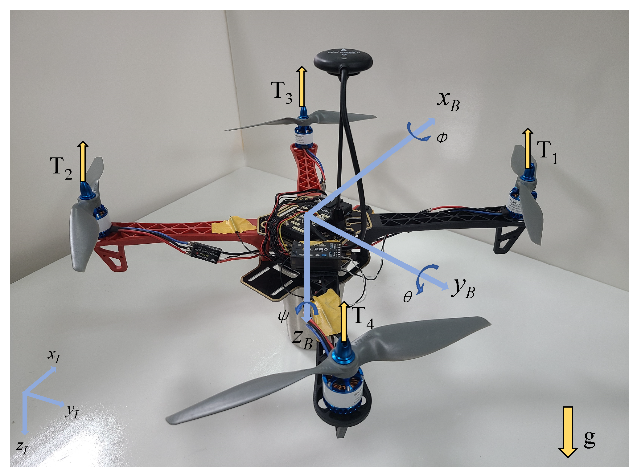
2.2.1. Attitude Motion Model of a Quadrotor Drone

In this work, the quadrotor drone is considered as a rigid body with an X-configuration. As illustrated in Figure 1, the rotational motion of the quadrotor drone is described in the inertial frame and the body-fixed frame, which are denoted as the I-frame and B-frame, respectively [40].

We adopt Euler angles $\mathbf{\Theta }={[\varphi ,\theta ,\psi ]}^T$ to represent the attitude of the quadrotor drone. $\varphi$, $\theta$, and $\psi$ represent the roll angle, pitch angle, and yaw angle, respectively.

Considering the rotation from I-frame to B-frame in the order of $\psi$–$\theta$–$\varphi$, the relationship between the Euler angle rates $\dot{\mathbf{\Theta }}$ and the body angular rate in B-frame $\mathit{\omega }={[{\omega }_x,{\omega }_y,{\omega }_z]}^T$ is formulated as the following nonlinear equations [41]:

$$\begin{array}{cc}\hfill & \dot{\varphi }={\omega }_x+{\omega }_{y}sin\varphi tan\theta +{\omega }_{z}cos\varphi tan\theta ,\hfill \\ \hfill & \dot{\theta }={\omega }_{y}cos\theta -{\omega }_{z}sin\varphi ,\hfill \\ \hfill & \dot{\psi }={\omega }_y\frac{sin\varphi }{cos\theta }+{\omega }_z\frac{cos\varphi }{cos\theta },\hfill \end{array}$$

(1)

In order to facilitate the subsequent control design, the nonlinear Equation (1) are rewritten in the linear form with disturbances:

$$\dot{\mathbf{\Theta }}=\mathit{\omega }+{\mathbf{f}}_{\Theta },$$

(2)

where

$${\mathbf{f}}_{\Theta }=\left[\begin{array}{c}{\omega }_{y}sin\varphi tan\theta +{\omega }_{z}cos\varphi tan\theta \\ {\omega }_y(cos\theta -1)-{\omega }_{z}sin\varphi \\ {\omega }_y\frac{sin\varphi }{cos\theta }+{\omega }_z(\frac{cos\varphi }{cos\theta }-1)\end{array}\right].$$

(3)

Remark 1.

In this work, Euler angles are employed to describe the attitude because they can be more directly mapped to the actual motion of the quadrotor drones, which is more intuitive and easier to understand than other representations [42,43]. Although the Euler angle representation suffers from the problem of gimbal lock [42,44], the configuration of quadrotor drones imposes constraints on the range of attitude angles. By carefully selecting the rotation order of the Euler angles, it is possible to prevent the occurrence of singularities.

Remark 2.

In the majority of existing studies, the lumped disturbance ${\mathbf{f}}_{\Theta }$ is overlooked based on the small angle approximation, leading to $\dot{\mathbf{\Theta }}\approx \mathit{\omega }$ [9,11,45]. However, with the increasing complexity of application scenarios and mission requirements, large angle maneuvers, where θ and ϕ deviate significantly from zero, become inevitable during the execution of aggressive missions for quadrotor drones. As a result, the small angle approximation is invalid and the kinematic coupling ${\mathbf{f}}_{\Theta }$ must be taken into consideration in the design process of attitude controllers.

The typical equation that represents the rotational dynamics of the quadrotor drone in B-frame is as follows [41]:

$$\mathbf{J}\dot{\mathit{\omega }}=-\mathit{\omega }\times \mathbf{J}\mathit{\omega }+\mathit{\tau }+{\mathbf{d}}_{\tau },$$

(4)

where $\mathbf{J}=diag\left([J_x,J_y,J_z]\right)$ is the quadrotor drone moment of inertia about its center of mass, which is positioned at the origin of the B-frame; ${\mathbf{d}}_{\tau }={[d_{\tau x},d_{\tau y},d_{\tau z}]}^T$ characterizes the external disturbance torque acting on the quadrotor drone, including the asymmetric torque, rotational inertia torque, and air-drag torque; $\mathit{\tau }={[{\tau }_x,{\tau }_y,{\tau }_z]}^T$ denotes the control torque with respect to the B-frame generated by the actuators, i.e., four rotors of the quadrotor drone. The components of $\mathit{\tau }$ are composed as

$$\begin{array}{cc}\hfill & {\tau }_x=\frac{\sqrt{2}}{2}l(-T_1+T_2+T_3-T_4),\hfill \\ \hfill & {\tau }_y=\frac{\sqrt{2}}{2}l(T_1-T_2+T_3-T_4),\hfill \\ \hfill & {\tau }_z=\frac{c_M}{c_T}(T_1+T_2-T_3-T_4),\hfill \end{array}$$

(5)

where l is the arm length of the quadrotor drone; $T_i(i=1,2,3,4)$ is the thrust generated by the ith rotor; $c_M$ and $c_T$ are two constant parameters of the rotors.

Rewriting Equation (4) into the linear form with lumped disturbances derives the following:

$$\mathbf{J}\dot{\mathit{\omega }}=\mathit{\tau }+{\mathbf{f}}_{\mathit{\omega }},$$

(6)

where

$${\mathbf{f}}_{\mathit{\omega }}={[f_{\omega x},f_{\omega y},f_{\omega z}]}^T=-\mathit{\omega }\times \mathbf{J}\mathit{\omega }+{\mathbf{d}}_{\tau }.$$

(7)

Please note that the torque $\mathit{\tau }$ is developed by the actuators, which possess inherent dynamics that affect their response to control inputs. These dynamics, in turn, impact the response and stability of the overall system. Our model includes the actuator dynamics to ensure more realistic and reliable analysis and control of the system. The FOPTD model is adopted to characterize the dynamics of the actuators. This model adequately represents the characteristics of the actuators, including bandwidth and time delay. Assuming the quadrotor drone with four identical rotors, the actuators in pitch, roll, and yaw channels exhibit identical dynamic characteristics. The specific form of the FOPTD actuator model is given by

$$T_a\dot{\mathit{\tau }}\left(t\right)=-\mathit{\tau }\left(t\right)+\mathbf{u}(t-t_d),T_a>0,t_d>0,$$

(8)

where $\mathbf{u}$ is the desired torque developed by the controller; the parameters $T_a$ and $t_d$ stand for the dynamic characteristics of the actuators and correspond to time constant and time delay, respectively.

Rewrite Equation (8) in a consistent form with Equations (2) and (6) as

$$T_a\dot{\mathit{\tau }}=-\mathit{\tau }+\mathbf{u}+{\mathbf{f}}_a,$$

(9)

where

$${\mathbf{f}}_a\left(t\right)=-\mathbf{u}\left(t\right)+\mathbf{u}(t-t_d).$$

(10)

Remark 3.

As is shown in [23,24], the parameters $T_a$ and $t_d$ can be accurately identified through offline identification methods. Therefore, in the subsequent controller design, the actuator model (8) can serve as a virtual sensor to estimate the output torque $\mathit{\tau }$ [23].

Up to this point, we have obtained the complete attitude motion model of the quadrotor drone which takes into account disturbances and actuator dynamics, composed of Equations (2), (6), and (9):

$$\begin{array}{cc}\hfill \dot{\mathbf{\Theta }}& =\mathit{\omega }+{\mathbf{f}}_{\Theta },\hfill \\ \hfill \mathbf{J}\dot{\mathit{\omega }}& =\mathit{\tau }+{\mathbf{f}}_{\mathit{\omega }},\hfill \\ \hfill T_a\dot{\mathit{\tau }}& =-\mathit{\tau }+\mathbf{u}+{\mathbf{f}}_a.\hfill \end{array}$$

(11)

2.2.2. Problem Statement

Considering both matched and mismatched disturbances as well as actuator dynamics, our goal is to devise a robust control law $\mathbf{u}$ for the quadrotor drone attitude motion system (11) that achieves ultimate bounded tracking of a desired attitude trajectory ${\Theta }_d$.

From Equation (11), it can be observed that the three attitude channels have an identical structure as the following three-order form:

$$\begin{array}{cc}\hfill & {\dot{x}}_1=x_2+f_1,\hfill \\ \hfill & J{\dot{x}}_2=x_3+f_2,\hfill \\ \hfill & T_a{\dot{x}}_3=-x_3+u+f_3,\hfill \end{array}$$

(12)

where, for the specific channel (pitch, roll or yaw channel), $x_1$, $x_1$, and $x_3$ represent the Euler angle, the angular velocity, and the actuator generating torque, respectively; $f_1$, $f_2$, and $f_3$ denote the lumped disturbances; J is the corresponding moment of inertia; u represents the input signal developed by the controller.

For simplicity, we designed the controller u for the three-order system (12) without losing generality. The specific controller for each channel simply needs to be identical to u, with appropriate adjustments made to the specific gains.

Thus, the control objective can be stated as designing a control law u for the system (12) to achieve ultimate boundedness for the tracking error, namely,

$$|x_{1d}-x_1|\le \delta ,\forall t>t_{\delta },$$

(13)

where $x_{1d}$ is the desired trajectory, $\delta >0$ denotes the ultimate bound of the tracking error, and $t_{\delta }$ is the corresponding settling time.

3. The HOSMDO-Based Control Strategy

In this section, a novel feedback control framework based on HOSMDO for the attitude tracking of system (12) is presented as shown in Figure 2.

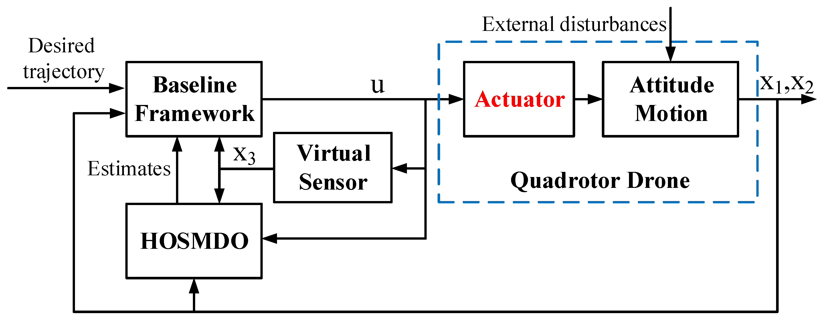
3.1. The Baseline Control Framework Design

Two virtual controls, $x_{2d}$ and $x_{3d}$, are introduced as the reference signals of $x_2$ and $x_3$, respectively. Then, the tracking errors are defined as

$$\begin{array}{cc}\hfill & e_1=x_{1d}-x_1,\hfill \\ \hfill & e_2=x_{2d}-x_2,\hfill \\ \hfill & e_3=x_{3d}-x_3.\hfill \end{array}$$

(14)

Combining the attitude dynamics (12) with the definitions (14) yields the error dynamics:

$$\begin{array}{cc}\hfill & {\dot{e}}_1=e_2-x_{2d}+{\dot{x}}_{1d}-f_1,\hfill \\ \hfill & J{\dot{e}}_2=e_3-x_{3d}+J{\dot{x}}_{2d}-f_2,\hfill \\ \hfill & T_a{\dot{e}}_3=-e_3-u+T_a{\dot{x}}_{3d}+x_{3d}-f_3.\hfill \end{array}$$

(15)

In (15), $x_{2d}$, $x_{3d}$, and u are the controls to be designed. However, the presence of derivatives ${\dot{x}}_{2d}$ and ${\dot{x}}_{3d}$ complicates the design. Motivated by idea of coordinate transformation in [23] and the feedback linearization technique, we introduce changes of control inputs as follows:

$$\begin{array}{cc}\hfill & u_1=x_{2d},\hfill \\ \hfill & u_2=x_{3d}-J{\dot{x}}_{2d},\hfill \\ \hfill & u_3=u-T_a{\dot{x}}_{3d}-x_{3d}.\hfill \end{array}$$

(16)

Then, the error dynamics (15) are converted to an equivalent linear system with disturbances in space-state form as

$$\mathbf{\Lambda }\dot{\mathbf{e}}=\mathbf{Ae}-\mathbf{u}-\mathbf{f},$$

(17)

where

$\mathbf{\Lambda }=\left[\begin{array}{ccc}1& 0& 0\\ 0& J& 0\\ 0& 0& T_a\end{array}\right]$, $\mathbf{e}=\left[\begin{array}{c}{e}_1\\ e_2\\ e_3\end{array}\right]$, $\mathbf{A}=\left[\begin{array}{ccc}0& 1& 0\\ 0& 0& 1\\ 0& 0& -1\end{array}\right]$, $\mathbf{u}=\left[\begin{array}{c}{u}_1\\ u_2\\ u_3\end{array}\right]$, and $\mathbf{f}=\left[\begin{array}{c}{f}_1-{\dot{x}}_{1d}\\ f_2\\ f_3\end{array}\right]$.

For stabilization, we design a state feedback control with disturbance compensation as

$$\mathbf{u}=\mathbf{\Lambda }\mathbf{K}\mathbf{e}-\mathbf{f},$$

(18)

and obtain the following closed-loop system:

$$\dot{\mathbf{e}}={\mathbf{A}}_1\mathbf{e},$$

(19)

where

$$\mathbf{K}=\left[\begin{array}{ccc}{k}_1& 0& 0\\ 0& k_2& 0\\ 0& 0& k_3\end{array}\right],{\mathbf{A}}_1={\mathbf{\Lambda }}^{-1}\mathbf{A}-\mathbf{K}=\left[\begin{array}{ccc}-k_1& 1& 0\\ 0& -k_2& \frac{1}{J}\\ 0& 0& -k_3-\frac{1}{T_a}\end{array}\right],$$

and $k_1$, $k_2$, and $k_3$ are the feedback gains to be selected.

According to Theorem 4.5 in [46], the asymptotic stability condition of the error dynamic system (17) with controller (18) is that ${\mathbf{A}}_1$ is a Hurwitz matrix, i.e.,

$$k_1>0,k_2>0,k_3>-\frac{1}{T_a}.$$

(20)

From (16) and (18), we can obtain the baseline control framework consisting of the following control inputs:

$$\begin{array}{cc}\hfill x_{2d}=& k_1{e}_1+{\dot{x}}_{1d}-f_1,\hfill \\ \hfill x_{3d}=& -{k_1}^{2}J{e}_1+\left(k_1+k_2\right)J{e}_2+J{\ddot{x}}_{1d}-f_2-J{\dot{f}}_1,\hfill \\ \hfill u=& \left(k_1{T}_a-1\right){k_1}^{2}J{e}_1-\left({k_1}^2+k_1{k}_2+{k_2}^2\right)T_{a}J{e}_2+\left(k_2+k_1\right)J{e}_2+\left(k_1+k_2+k_3\right)T_a{e}_3\hfill \\ \hfill & +J{\ddot{x}}_{1d}+T_{a}J{\stackrel{⃛}{x}}_{1d}-f_2-f_3-J{\dot{f}}_1-T_a{\dot{f}}_2-T_{a}J{\ddot{f}}_1.\hfill \end{array}$$

(21)

However, the disturbances $f_1$, $f_2$, and $f_3$ and their derivatives ${\dot{f}}_1$, ${\ddot{f}}_1$, and ${\dot{f}}_2$ are immeasurable, which leads to the inability of the controller (21) to be applied. For this reason, we propose a HOSMDO to estimate the disturbances and their arbitrary order derivatives exactly.

3.2. The High-Order Sliding Mode Disturbance Observer

Consider a class of system with disturbance as follows:

$$ϵ\dot{x}=g(x,u)+f\left(t\right),$$

(22)

where $ϵ$ is a known positive constant, $g(x,u)$ is a known function, and $f\left(t\right)$ is an unknown disturbance that is assumed to be nth differentiable with a Lipschitz constant $L>0$, i.e., $|\frac{d^n}{d{t}^n}f\left(t\right)|\le L$.

Motivated by the extended state observer technique, the following auxiliary variables are defined:

$$\begin{array}{cc}\hfill & z_i=f^{(i-1)}\left(t\right),i=1,2,\cdots ,n,\hfill \\ \hfill & H=f^{\left(n\right)}\left(t\right),\hfill \end{array}$$

(23)

where $f^{\left(i\right)}\left(t\right)\triangleq \frac{d^i}{d{t}^i}f\left(t\right)$. Then, we can rewrite (22) in the extended state form:

$$\begin{array}{cc}\hfill & {\dot{z}}_0=g(x,u)+z_1,\hfill \\ \hfill & {\dot{z}}_i=z_{i+1},i=1,2,\cdots ,n-1,\hfill \\ \hfill & {\dot{z}}_n=H,\hfill \end{array}$$

(24)

where $z_0\triangleq ϵx$ for convenience of expression.

Let ${\widehat{z}}_i$ represent the estimate of $z_i(i=0,1,\cdots ,n)$. Inspired by the original HOSM differentiator with finite-time convergence in [29], the HOSMDO is designed to obtain the estimates of the disturbance f and its successive derivatives $f^{\left(i\right)}(i=1,\cdots ,n-1)$, which is given by

$$\begin{array}{cc}\hfill & {\dot{\widehat{z}}}_0=g(x,u)+{\widehat{z}}_1-{\beta }_0{\lfloor {\widehat{z}}_0-z_0\rceil }^{\frac{n}{n+1}},\hfill \\ \hfill & {\dot{\widehat{z}}}_i={\widehat{z}}_{i+1}-{\beta }_i{\lfloor {\widehat{z}}_0-z_0\rceil }^{\frac{n-i}{n+1}},i=1,2,\cdots ,n-1,\hfill \\ \hfill & {\dot{\widehat{z}}}_n=-{\beta }_{n}sign({\widehat{z}}_0-z_0),\hfill \end{array}$$

(25)

where ${\beta }_i(i=0,1,\cdots ,n)$ are the coefficients to be selected, and ${\lfloor a\rceil }^b$ is the abbreviation for

$${\lfloor a\rceil }^b\triangleq {\left|a\right|}^{b}sign\left(a\right),a,b\in \mathbb{R}.$$

(26)

All three formulas in (12) satisfy the format of (22). By setting n to 3, 2, and 2, respectively, the following observers can be obtained to estimate the unknown disturbances and the derivatives present in the baseline control framework (21):

$$HOSMDO1:\left\{\begin{array}{c}{\dot{\widehat{x}}}_1=x_2+{\widehat{f}}_1-{\beta }_0^1{\lfloor {\widehat{x}}_1-x_1\rceil }^{\frac{3}{4}},\hfill \\ {\dot{\widehat{f}}}_1={\widehat{\dot{f}}}_1-{\beta }_1^1{\lfloor {\widehat{x}}_1-x_1\rceil }^{\frac{2}{4}},\hfill \\ {\dot{\widehat{\dot{f}}}}_1={\widehat{\ddot{f}}}_1-{\beta }_2^1{\lfloor {\widehat{x}}_1-x_1\rceil }^{\frac{1}{4}},\hfill \\ {\dot{\widehat{\ddot{f}}}}_1=-{\beta }_3^{1}sign({\widehat{x}}_1-x_1),\hfill \end{array}\right.$$

(27)

$$HOSMDO2:\left\{\begin{array}{c}J{\dot{\widehat{x}}}_2=x_3+{\widehat{f}}_2-{\beta }_0^2{\lfloor J{\widehat{x}}_2-J{x}_2\rceil }^{\frac{2}{3}},\hfill \\ {\dot{\widehat{f}}}_2={\widehat{\dot{f}}}_2-{\beta }_1^2{\lfloor J{\widehat{x}}_2-J{x}_2\rceil }^{\frac{1}{3}},\hfill \\ {\dot{\widehat{\dot{f}}}}_2=-{\beta }_2^{2}sign(J{\widehat{x}}_2-J{x}_2),\hfill \end{array}\right.$$

(28)

$$HOSMDO3:\left\{\begin{array}{c}{T}_a{\dot{\widehat{x}}}_3=-x_3+u+{\widehat{f}}_3-{\beta }_0^3{\lfloor T_a{\widehat{x}}_3-T_a{x}_3\rceil }^{\frac{2}{3}},\hfill \\ {\dot{\widehat{f}}}_3={\widehat{\dot{f}}}_3-{\beta }_1^3{\lfloor T_a{\widehat{x}}_3-T_a{x}_3\rceil }^{\frac{1}{3}},\hfill \\ {\dot{\widehat{\dot{f}}}}_3=-{\beta }_2^{3}sign(T_a{\widehat{x}}_3-T_a{x}_3),\hfill \end{array}\right.$$

(29)

where ${\widehat{x}}_1$, ${\widehat{x}}_2$, ${\widehat{x}}_3$, ${\widehat{f}}_1$, ${\widehat{\dot{f}}}_1$, ${\widehat{\ddot{f}}}_1$, ${\widehat{f}}_2$, ${\widehat{\dot{f}}}_2$, and ${\widehat{f}}_3$ are the estimates of $x_1$, $x_2$, $x_3$, $f_1$, ${\dot{f}}_1$, ${\ddot{f}}_1$, $f_2$, ${\dot{f}}_2$, and $f_3$, respectively, and ${\beta }_i^j(j=1,2,3,i=0,1,2,3)$ are the coefficients.

Remark 4.

It can be observed in (21) that $f_3$ is introduced into u without any scaling, which directly links the performance of estimating $f_3$ to the behavior of u. In order to achieve better estimation accuracy of $f_3$ and lower sensitivity to chattering, HOSMDO3 (29) is designed with a third-order structure rather than a second-order one, even though the latter can theoretically provide an estimate of $f_3$.

3.3. The Proposed Control Strategy

Substituting the unknown disturbances $f_1$, $f_2$, and $f_3$ and the derivatives ${\dot{f}}_1$, ${\ddot{f}}_1$, and ${\dot{f}}_2$ in the baseline control framework (21) with the corresponding estimated signals generated by the HOSMDOs (27)–(29), the proposed HOSMDO-based control scheme is expressed as

$$\begin{array}{cc}\hfill x_{2d}=& k_1{e}_1+{\dot{x}}_{1d}-{\widehat{f}}_1,\hfill \\ \hfill x_{3d}=& -{k_1}^{2}J{e}_1+\left(k_1+k_2\right)J{e}_2+J{\ddot{x}}_{1d}-{\widehat{f}}_2-J{\widehat{\dot{f}}}_1,\hfill \\ \hfill u=& \left(k_1{T}_a-1\right){k_1}^{2}J{e}_1-\left({k_1}^2+k_1{k}_2+{k_2}^2\right)T_{a}J{e}_2+\left(k_2+k_1\right)J{e}_2+\left(k_1+k_2+k_3\right)T_a{e}_3\hfill \\ \hfill & +J{\ddot{x}}_{1d}+T_{a}J{\stackrel{⃛}{x}}_{1d}-{\widehat{f}}_2-{\widehat{f}}_3-J{\widehat{\dot{f}}}_1-T_a{\widehat{\dot{f}}}_2-T_{a}J{\widehat{\ddot{f}}}_1.\hfill \end{array}$$

(30)

The newly proposed control strategy, combining the state feedback control with disturbance compensation, is designed with a holistic mindset for the entire system (12) suffering from matched and mismatched disturbances. The design process consists of two main steps:

• construct a baseline framework in the ideal scenario where all disturbance information is known;
• replace the disturbances and relevant derivatives required for the baseline framework with the corresponding estimates generated by the HOSMDOs to obtain the overall control scheme.

4. Stability Analysis

4.1. Analysis of HOSMDO

Defining the estimation errors of the HOSMDO (25) as

$${\tilde{z}}_i={\widehat{z}}_i-z_i,i=0,1,\cdots ,n,$$

(31)

we can derive the error dynamics:

$$\begin{array}{cc}\hfill & {\dot{\tilde{z}}}_i=-{\beta }_i{\lfloor {\tilde{z}}_0\rceil }^{\frac{n-i}{n+1}}+{\tilde{z}}_{i+1},i=0,1,\cdots ,n-1,\hfill \\ \hfill & {\dot{\tilde{z}}}_n=-{\beta }_{n}sign\left({\tilde{z}}_0\right)-H.\hfill \end{array}$$

(32)

Lemma 1.

For the system (22), if the HOSMDO (25) is designed to estimate the disturbance $f\left(t\right)$ and its successive derivatives $f^{\left(i\right)}(i=1,\cdots ,n-1)$, there are positive values of ${\beta }_i(i=0,1,\cdots ,n-1)$ and ${\beta }_n>L$ such that the estimation errors ${\tilde{z}}_1,{\tilde{z}}_2,\cdots ,{\tilde{z}}_n$ converge to zero in finite time.

The following theoretical proof of Lemma 1 is inspired by the Lyapunov approach proposed in [39].

Proof of Lemma 1.

Note that the system (32) is homogeneous with degree $d=-1$ associated with the dilation $\mathbf{r}=(n+1,n,\cdots ,1)$. To facilitate the subsequent expression, we use $r_i(i=0,1,\cdots ,n)$ to represent the $(i+1)$th component of $\mathbf{r}$. Executing the change of coordinate as follows:

$${\zeta }_0={\tilde{z}}_0,{\zeta }_1=\frac{{\tilde{z}}_1}{{\beta }_0},\cdots ,{\zeta }_i=\frac{{\tilde{z}}_i}{{\beta }_{i-1}},\cdots ,{\zeta }_n=\frac{{\tilde{z}}_n}{{\beta }_{n-1}},$$

(33)

the error dynamics (32) can be rewritten as

$$\begin{array}{cc}\hfill & {\dot{\zeta }}_i={\alpha }_i\left(-{\lfloor {\zeta }_0\rceil }^{\frac{r_{i+1}}{r_0}}+{\zeta }_{i+1}\right),i=0,\cdots ,n-1,\hfill \\ \hfill & {\dot{\zeta }}_n=-{\alpha }_n\mathrm{sign}\left({\zeta }_0\right)-\overline{H},\hfill \end{array}$$

(34)

where ${\alpha }_0={\beta }_0$, ${\alpha }_i=\frac{{\beta }_i}{{\beta }_{i-1}},i=1,2,\cdots ,n$, and $\overline{H}=\frac{H}{{\beta }_{n-1}}$.

For $n\ge 1$, we select a constant p which satisfies $p\ge r_0+r_1=2n+1$. We define the following homogeneous functions:

$$Z_i\left({\zeta }_i,{\zeta }_{i+1}\right)=\frac{r_i}{p}{\left|{\zeta }_i\right|}^{\frac{p}{r_i}}-{\zeta }_i{⌊{\zeta }_{i+1}⌉}^{\frac{p-r_i}{r_{i+1}}}+\frac{p-r_i}{p}{\left|{\zeta }_{i+1}\right|}^{\frac{p}{r_{i+1}}},i=0,\cdots ,n-1.$$

(35)

Let us introduce the following Lyapunov function:

$$V\left(\mathit{\zeta }\right)=\sum _{j=0}^{n-1}{\rho }_j{Z}_j\left({\zeta }_j,{\zeta }_{j+1}\right)+{\rho }_n\frac{1}{p}{\left|{\zeta }_n\right|}^p,$$

(36)

where ${\rho }_i>0(i=0,\cdots ,n)$.

According to the proofs of Theorem 3 and Theorem 4 in [39], $V\left(\mathit{\zeta }\right)$ is positive definite, and there are positive values of ${\beta }_i(i=0,1,\cdots ,n-1)$ and ${\beta }_n>L$ such that $\dot{V}\left(\mathit{\zeta }\right)$ is negative. Therefore, the origin of the error dynamics system (32) is asymptotically stable by Lyapunov’s stability theorem (see Theorem 4.1 in [46]). Applying Theorem 8 in [30], the origin of the system (32) is finite-time stable, i.e., the estimation errors ${\tilde{z}}_1,{\tilde{z}}_2,\cdots ,{\tilde{z}}_n$ converge to zero in finite time. □

Remark 5.

The advantage of the proposed HOSMDO lies in its capability to estimate high-order time-varying matched/mismatched disturbances and their higher-order derivatives, with the estimation error converging to zero within a finite time. Specifically, different from other disturbance observers such as UDE and ESO, HOSMDO can estimate the various derivatives of disturbances, rather than just obtaining an estimate of the disturbance itself. Therefore, by adequately compensating for the derivatives of high-order time-varying disturbances in the controller, the disturbance rejection capability and control accuracy can be enhanced.

The following assumption is imposed for the system (12).

Assumption 1.

$\stackrel{⃛}{f_1}$, $\ddot{f_2}$, and $\ddot{f_3}$ are bounded.

Under Assumption 1, the estimates generated by the HOSMDOs (27)–(29), i.e., ${\widehat{f}}_1$, ${\widehat{\dot{f}}}_1$, ${\widehat{\ddot{f}}}_1$, ${\widehat{f}}_2$, ${\widehat{\dot{f}}}_2$, and ${\widehat{f}}_3$, converge to their respective true values, i.e., $f_1$, ${\dot{f}}_1$, ${\ddot{f}}_1$, $f_2$, ${\dot{f}}_2$, and $f_3$, within a finite time according to Lemma 1.

4.2. Analysis of the Proposed Controller

Combining the system (15) with the proposed controller (30) yields the closed-loop tracking error dynamics:

$$\begin{array}{cc}\hfill & {\dot{e}}_1=-k_1{e}_1+e_2+{\tilde{f}}_1,\hfill \\ \hfill & {\dot{e}}_2=-k_2{e}_2+\frac{1}{J}{e}_3+\frac{1}{J}{\tilde{f}}_2+k_1{\tilde{f}}_1+{\widehat{\dot{f}}}_1-{\dot{\widehat{f}}}_1,\hfill \\ \hfill & {\dot{e}}_3=-k_3{e}_3-\frac{1}{T_a}{e}_3+\frac{1}{T_a}{\tilde{f}}_3+\left(k_2+k_1\right){\tilde{f}}_2+J\left(k_2+k_1\right)\left({\widehat{\dot{f}}}_1-{\dot{\widehat{f}}}_1\right)+J\left({\widehat{\ddot{f}}}_1-{\dot{\widehat{\dot{f}}}}_1\right)+{\widehat{\dot{f}}}_2-{\dot{\widehat{f}}}_2,\hfill \end{array}$$

(37)

where ${\tilde{f}}_i\triangleq {\widehat{f}}_i-f_i(i=1,2,3)$.

Let us rephrase (37) into the state-space form

$$\dot{\mathbf{e}}={\mathbf{A}}_1\mathbf{e}+{\mathbf{f}}_l,$$

(38)

where

$${\mathbf{f}}_l=\left[\begin{array}{cc}& {\tilde{f}}_1\\ & \frac{1}{J}{\tilde{f}}_2+k_1{\tilde{f}}_1+{\widehat{\dot{f}}}_1-{\dot{\widehat{f}}}_1\\ & \frac{1}{T_a}{\tilde{f}}_3+\left(k_2+k_1\right){\tilde{f}}_2+J\left(k_2+k_1\right)\left({\widehat{\dot{f}}}_1-{\dot{\widehat{f}}}_1\right)+J\left({\widehat{\ddot{f}}}_1-{\dot{\widehat{\dot{f}}}}_1\right)+{\widehat{\dot{f}}}_2-{\dot{\widehat{f}}}_2\end{array}\right].$$

Remark 6.

Considering ${\mathbf{f}}_l$ as the input to the system (38), we can observe that the unforced system is identical to the system (19). Note that (19) is the closed-loop error dynamics obtained based on the baseline control framework. Thus, the effect of the disturbance estimation error generated by the HOTFESOs is only present in the system input ${\mathbf{f}}_l$. This property supports the two-step design procedure we proposed, enabling us to design the baseline framework and HOSMDOs separately.

Theorem 1.

Under Assumption 1, if the condition (20) is satisfied, the error dynamic system (38) with ${\mathbf{f}}_l$ as input is input-to-state stable (ISS) and the tracking error $e_1$ is globally bounded.

Proof. 

For the error dynamic system (38), by ensuring the feedback gains satisfy the condition (20), the matrix ${\mathbf{A}}_1$ is Hurwitz such that the origin of the unforced system $\dot{\mathbf{e}}={\mathbf{A}}_1\mathbf{e}$ is globally exponentially stable. Due to Lemma 4.6 in [46], the system (38) is ISS with respect to ${\mathbf{f}}_l$.

According to Lemma 1, if the parameters are properly selected, the estimation errors of the HOSMDOs are finite-time stable, i.e., ${\tilde{f}}_1$, ${\tilde{f}}_2$, and ${\tilde{f}}_3$ converge to zero in finite time. Moreover, from Equations (27)–(29), we can derive that the discrepancies ${\widehat{\dot{f}}}_1-{\dot{\widehat{f}}}_1$,${\widehat{\ddot{f}}}_1-{\dot{\widehat{\dot{f}}}}_1$, and ${\widehat{\dot{f}}}_2-{\dot{\widehat{f}}}_2$ tend to zero in finite time as well.

The solution of the differential Equation (38) is written as

$$\mathbf{e}\left(t\right)=e^{t{\mathbf{A}}_1}\mathbf{e}\left(0\right)+{\int }_0^t{e}^{(t-\tau ){\mathbf{A}}_1}{\mathbf{f}}_l\left(\tau \right)d\tau .$$

(39)

It is evident that the zero-input response decays to zero exponentially, while the zero-state response is bounded since the terms contained in ${\mathbf{f}}_l\left(\tau \right)$ are all bounded and converge to zero in finite time. Thus, the solution $\mathbf{e}\left(t\right)$ is globally bounded and the tracking error $e_1$, as a component of $\mathbf{e}$, is also globally bounded. □

4.3. Analysis of the Reduced Controller

Next, we will investigate how the system stability will be affected by applying the same design process as the proposed controller when neglecting the actuators.

By ignoring the actuator dynamics, i.e., considering $x_3=u$, the reduced system corresponding to the full system (12) is given by

$$\begin{array}{cc}\hfill & {\dot{x}}_1=x_2+f_1,\hfill \\ \hfill & J{\dot{x}}_2=u+f_2.\hfill \end{array}$$

(40)

Based on the reduced system (40) and employing the same design process as (30), we obtain the reduced controller as shown below:

$$\begin{array}{cc}\hfill x_{2d}=& k_1{e}_1+{\dot{x}}_{1d}-{\widehat{f}}_1,\hfill \\ \hfill u=& -{k_1}^{2}J{e}_1+\left(k_1+k_2\right)J{e}_2+J{\ddot{x}}_{1d}-{\widehat{f}}_2-J{\widehat{\dot{f}}}_1.\hfill \end{array}$$

(41)

Note that by setting $T_a=0$ and $f_3=0$, the proposed controller (30) is identical to the reduced controller (41). In this case, it yields that $x_{3d}=u$. Combining (41) with the actual system (12) derives the tracking error dynamics

$$\dot{\mathbf{e}}={\mathbf{A}}_2\mathbf{e}+{\mathbf{f}}_{lr},$$

(42)

where

$${\mathbf{A}}_2=\left[\begin{array}{ccc}-k_1& 1& 0\\ 0& -k_2& \frac{1}{J}\\ J{k_1}^3& -J({k_1}^2+k_1{k}_2+{k_2}^2)& k_1+k_2-\frac{1}{T_a}\end{array}\right],$$

and

$${\mathbf{f}}_{lr}=\left[\begin{array}{cc}& {\tilde{f}}_1\\ & \frac{1}{J}{\tilde{f}}_2+k_1{\tilde{f}}_1+{\widehat{\dot{f}}}_1-{\dot{\widehat{f}}}_1\\ & J{k}_1{k}_2{\tilde{f}}_1+\left(k_2+k_1\right){\tilde{f}}_2+J\left(k_2+k_1\right)\left({\widehat{\dot{f}}}_1-{\dot{\widehat{f}}}_1\right)-J{\dot{\widehat{\dot{f}}}}_1-{\dot{\widehat{f}}}_2-\frac{1}{T_a}{f}_3+J{\stackrel{⃛}{x}}_{1d}\end{array}\right].$$

We can obtain the characteristic polynomial of ${\mathbf{A}}_2$ as

$$|s\mathbf{I}-{\mathbf{A}}_2|=s^3+\frac{1}{T_a}{s}^2+\frac{1}{T_a}\left(k_1+k_2\right)s+\frac{1}{T_a}{k}_1{k}_2.$$

(43)

From Routh criterion, ${\mathbf{A}}_2$ is Hurwitz if and only if the following stability conditions are satisfied:

$$\left\{\begin{array}{cc}\hfill & k_1>0,\hfill \\ \hfill & k_2>0,\hfill \\ \hfill & \frac{1}{k_1}+\frac{1}{k_2}>T_a.\hfill \end{array}\right.$$

(44)

Then, the system (42) with ${\mathbf{f}}_{lr}$ as input is ISS under the conditions (44) by Lemma 4.6 in [46].

A comparison of (20) and (44) shows that, if the actuator dynamics are neglected during controller design, there is an additional constraint on the allowable values of feedback gains $k_1$ and $k_2$ in relation to the actuator parameter $T_a$. Specifically, this constraint limits the upper bounds of $k_1$ and $k_2$.

Comparing conditions (44) with (20), it can be observed that, in the reduced case, actuator dynamics imposes an additional constraint on the feedback gains $k_1$ and $k_2$, which is related to the actuator parameter $T_a$. Specifically, this constraint indicates that the actuator parameter $T_a$ restricts the upper limits of the controller parameters $k_1$ and $k_2$. In addition, by comparing ${\mathbf{f}}_l$ in the system (38) with ${\mathbf{f}}_{lr}$ in the system (42), it is observed that all terms in ${\mathbf{f}}_l$ converge to zero within a finite time, whereas in ${\mathbf{f}}_{lr}$, there is $-J{\dot{\widehat{\dot{f}}}}_1-{\dot{\widehat{f}}}_2-\frac{1}{T_a}{f}_3+J{\stackrel{⃛}{x}}_{1d}$ that do not converge to zero. Therefore, neglecting the actuator dynamics in the controller design process would result in uncertainties such as actuator uncertainty $f_3$, reference trajectory information ${\stackrel{⃛}{x}}_{1d}$, and estimates of model disturbances ${\dot{\widehat{\dot{f}}}}_1$ and ${\dot{\widehat{f}}}_2$ affecting the tracking error range of the closed-loop system, thereby impacting the overall control precision.

Remark 7.

In feedback control, a larger gain leads to closed-loop poles farther away from the imaginary axis, resulting in faster system response. However, the presence of the actuator time constant $T_a$ limits the upper bounds of the feedback gains, indicating that the speed of the outer loop system is constrained by the actuator dynamics, aligning with common engineering knowledge. In the intelligent controller design presented in this chapter, the constraints mentioned above are eliminated by fully utilizing the dynamic model of the actuator.

5. Simulation Results

This section presents the simulation results to illustrate the main ideas of this work. Specifically, a comparison with respect to the CMUDE-based controller [24] is provided to validate the effectiveness of the proposed HOSMDO-based control strategy. In addition, a comparative study is conducted between the proposed controller (30) and the reduced controller (41) to showcase the importance of considering non-ideal actuator dynamics in the controller design.

In the simulation, the parameters of the quadrotor drone attitude motion model are $J_x=0.1025\mathrm{kg}·{\mathrm{m}}^2$, $J_y=0.0859\mathrm{kg}·{\mathrm{m}}^2$, $J_z=0.115\mathrm{kg}·{\mathrm{m}}^2$, $T_a=0.1\mathrm{s}$, and $t_d=0.04\mathrm{s}$. As depicted in Figure 3, the desirable attitude trajectories are considered as ${\varphi }_d=0deg$, ${\theta }_d=30sin\left(\frac{2\pi }{10}t\right)deg$, and ${\psi }_d=\left\{\begin{array}{cc}0deg,\hfill & t<16\mathrm{s},\hfill \\ 5deg,\hfill & 16\mathrm{s}\le t<32\mathrm{s}\hfill \\ 10sin\left(\frac{2\pi }{8}t\right)deg,\hfill & t\ge 32\mathrm{s},\hfill \end{array}\right.$. Furthermore, we add external disturbance torques as ${\mathbf{d}}_{\tau }={[0.05,-0.05,0.05]}^T\mathrm{N}·\mathrm{m}$. The simulation initial parameters are set to ${\varphi }_0={\theta }_0={\psi }_0=0deg$ and ${\omega }_{x0}={\omega }_{y0}={\omega }_{z0}=0deg/\mathrm{s}$. All three attitude channels are considered to share the same group of controller parameters, which are displayed in

Table 1. Default controller parameters.

Proposed Controller								CMUDE-Based Controller
$k_1$	2	${\beta }_0^1$	−10	${\beta }_0^2$	−1	${\beta }_0^3$	−1	$c_1$	2	$T_{\theta }$	0.5
$k_2$	8	${\beta }_1^1$	−100	${\beta }_1^2$	−1	${\beta }_1^3$	−0.1	$c_2$	1	$T_p$	0.2
$k_3$	10	${\beta }_2^1$	−100	${\beta }_2^2$	−0.1	${\beta }_2^3$	−0.01	$c_3$	1	$T_m$	0.05
		${\beta }_3^1$	−30

.

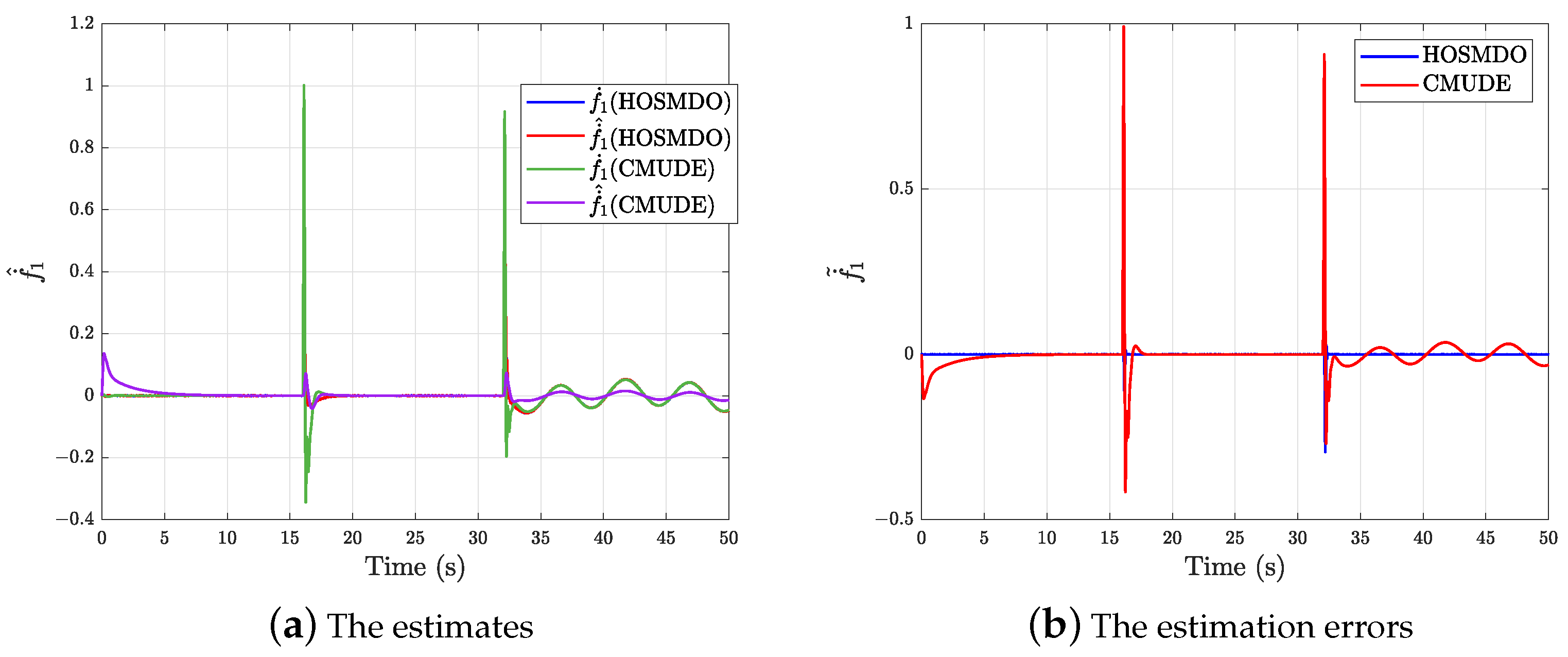
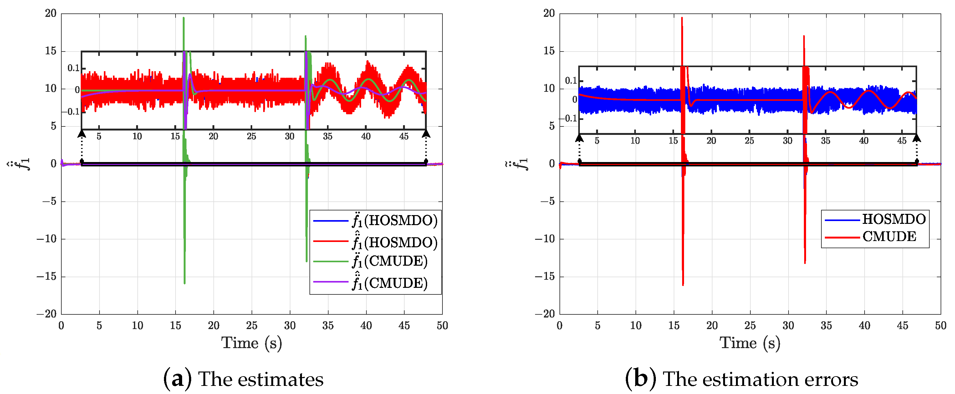
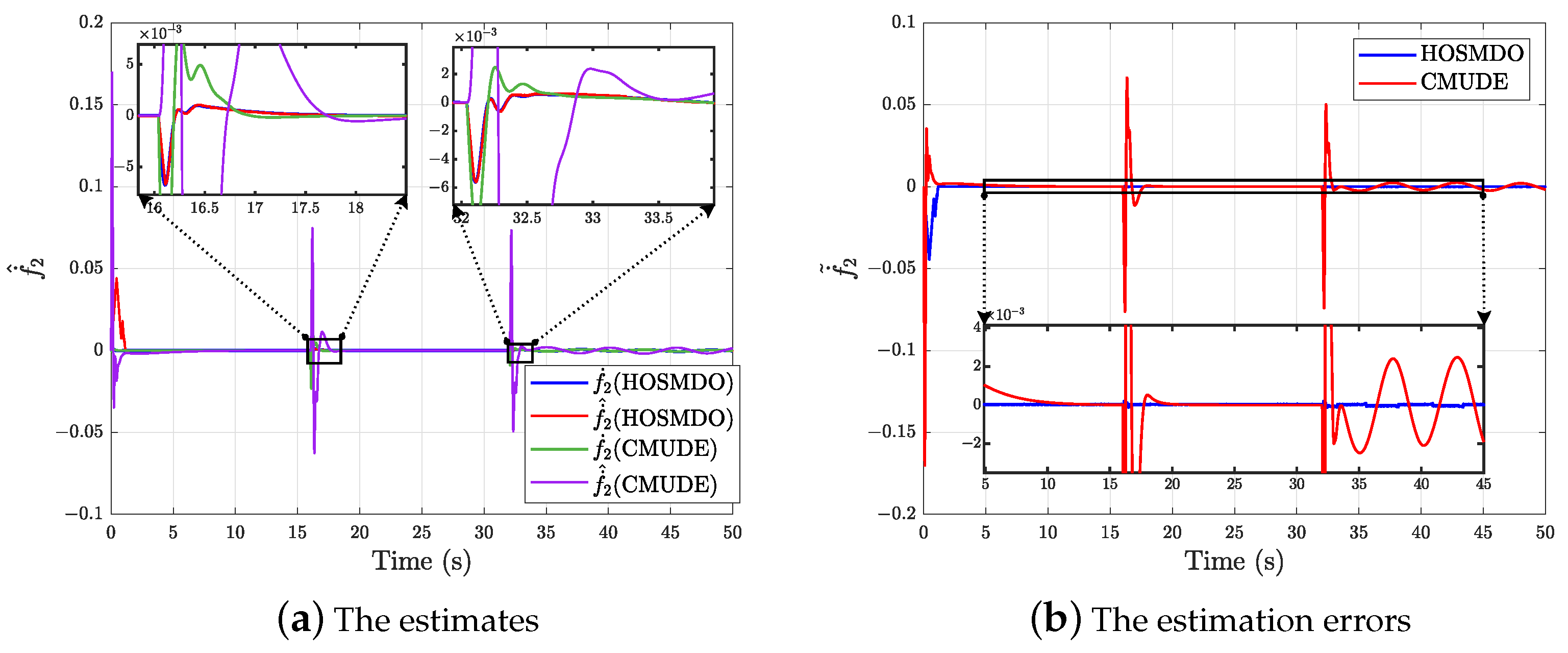
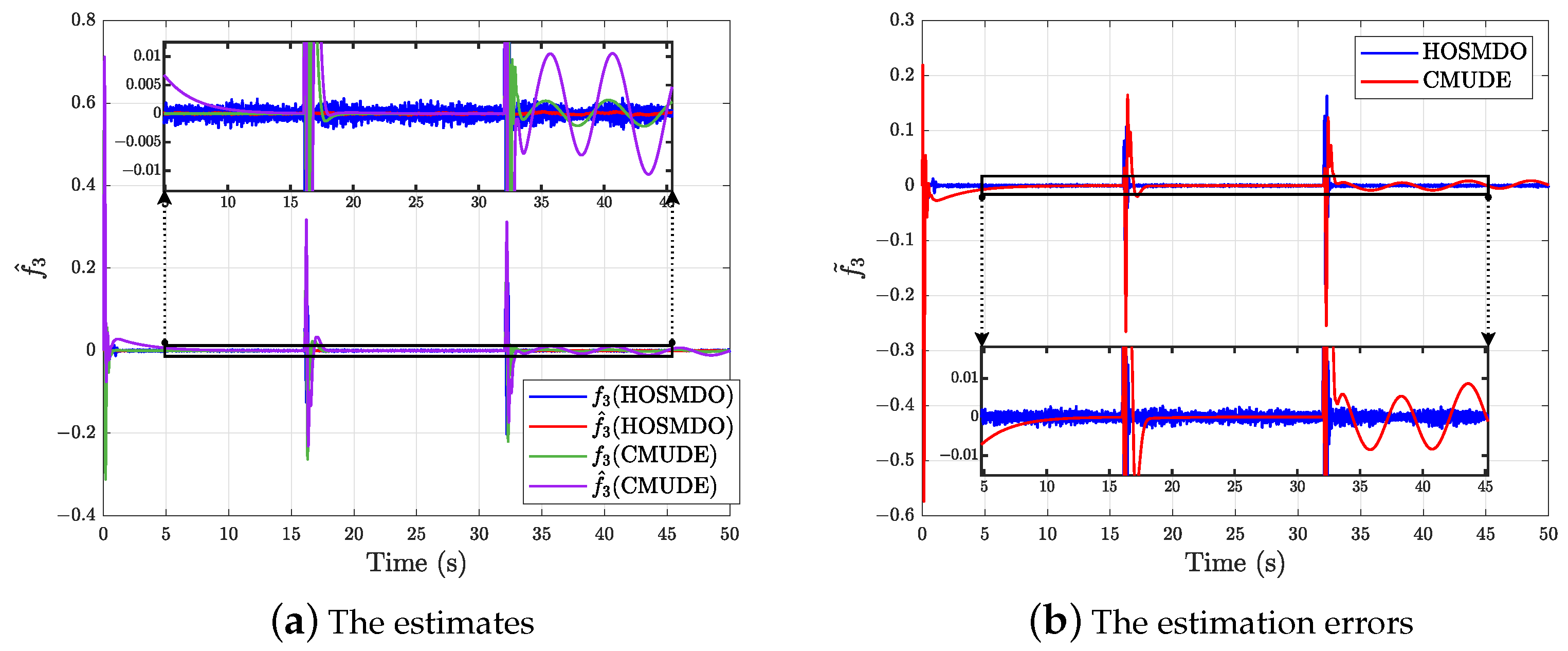
5.1. Comparison Results for the Proposed Controller and the CMUDE-Based Controller

The comparison results of attitude tracking errors and disturbance estimation errors generated by the proposed HOSMDO-based controller and the CMUDE-based controller are shown in Figure 4, Figure 5, Figure 6, Figure 7, Figure 8, Figure 9 and Figure 10.

In accordance with Figure 4,

Table 2. RMS of attitude tracking errors.

		$\mathbf{RMS}\left(\tilde{\mathit{\varphi }}\right)$	$\mathbf{RMS}\left(\tilde{\mathit{\theta }}\right)$	$\mathbf{RMS}\left(\tilde{\mathit{\psi }}\right)$
Proposed controller		0.0024	0.0010	0.0015
CMUDE-based controller		0.3338	0.0947	0.0793

shows the Root Mean Square (RMS) of the attitude tracking errors for the three channels in the interval from 40 s to 50 s. From Figure 4 and Table 2, it can be observed that the steady-state tracking error of the proposed controller is significantly smaller compared to the CMUDE-based controller. Additionally, at simulation times of 16 s and 32 s, when the reference signal undergoes non-continuous changes, the proposed controller produces smoother transient behavior of tracking errors compared to the CMUDE-based controller. These findings highlight the superiority of the proposed controller in accurately and effectively controlling the attitude of the system.

Figure 5, Figure 6, Figure 7, Figure 8, Figure 9 and Figure 10 show that both HOSMDO and CMUDE achieve high-precision estimation for constant signals (simulated from 0 s to 32 s). However, for time-varying signals (occurring from 32 s to 50 s), HOSMDO exhibits higher estimation accuracy. In addition, in response to the abrupt changes at 16 s and 32 s, CMUDE generates significantly larger transient overshoot compared to HOSMDO. These findings corroborate that HOSMDO is less sensitive to signal transients, is more accurate in capturing signal dynamics, and exhibits greater robustness due to its sliding mode properties.

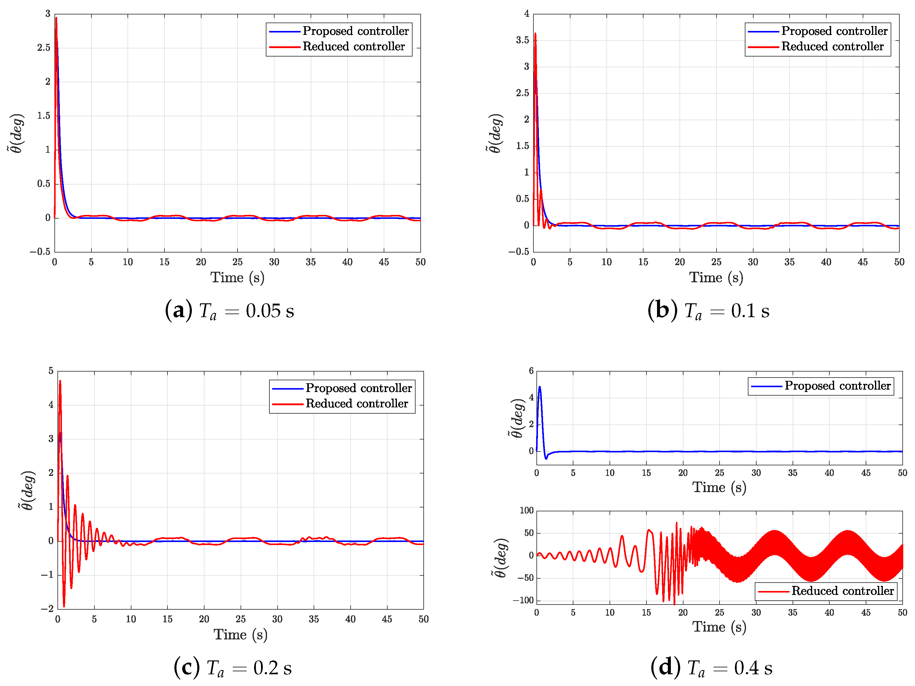
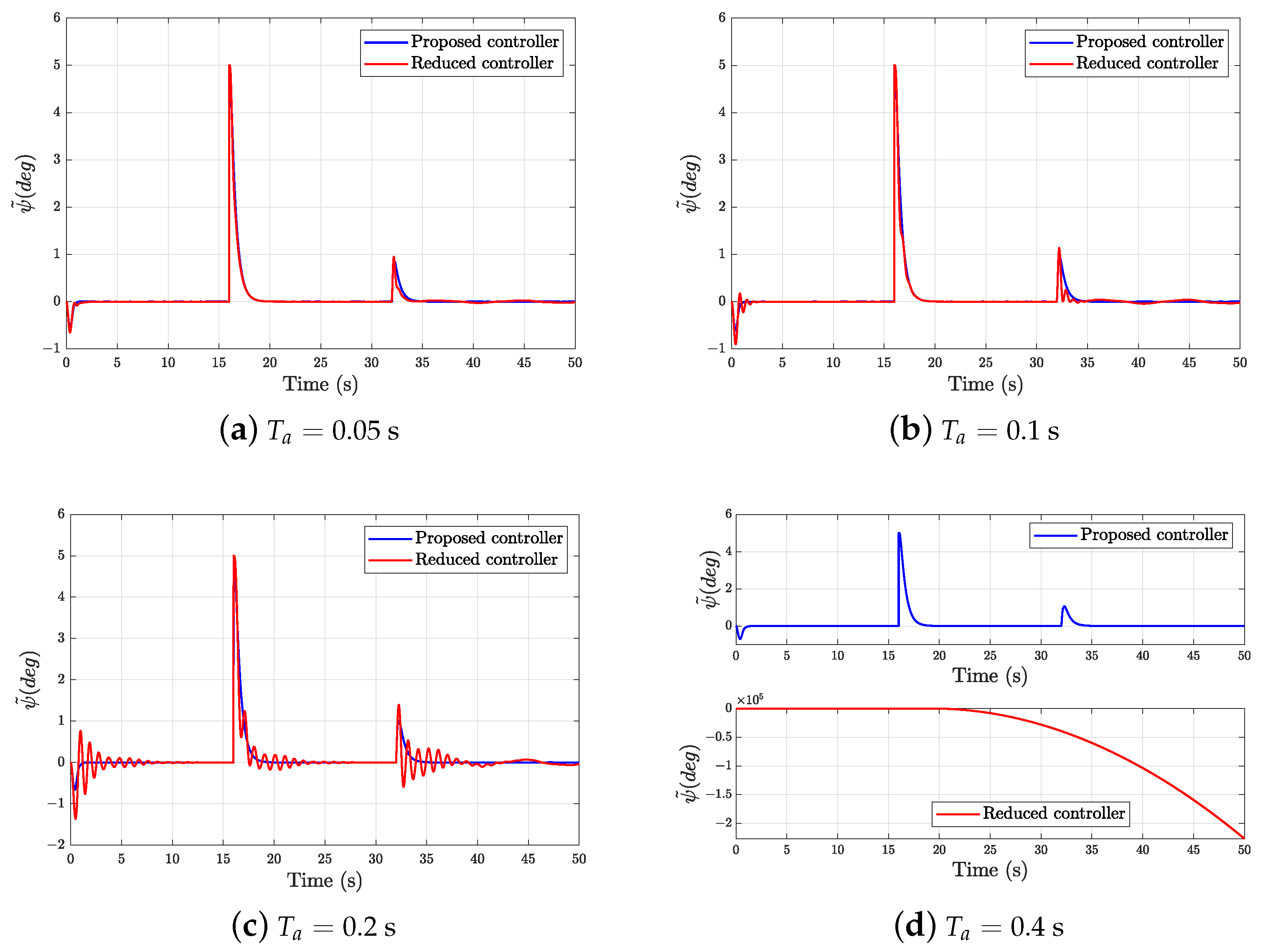
5.2. Comparison Results for the Proposed Controller and the Reduced Controller

Figure 11, Figure 12 and Figure 13 illustrate the attitude tracking error results of three channels for the proposed controller (with actuator dynamics considerations) and the reduced controller (without actuator dynamics considerations) under different actuator time constants $T_a$. As shown in Figure 11, Figure 12 and Figure 13, at the same $T_a$, the reduced controller has poorer tracking performance compared to the proposed controller, with larger overshoot and stronger oscillations. Additionally, as $T_a$ increases, the control effectiveness of the reduced controller deteriorates, eventually leading to instability. This highlights the importance of considering actuator dynamics in the controller design process. The aggregated results of the proposed controller under different $T_a$ values are presented in Figure 14. It can be observed that the errors vary slightly under different $T_a$ values, showcasing strong robustness of the proposed controller in handling actuator dynamics.

6. Conclusions

In this paper, a control strategy combining state feedback control with HOSMDO is proposed to address the challenges of attitude tracking in quadrotor drones. The holistic design of the controller, integrating a baseline feedback framework with disturbance estimation, contributes to an intuitive and comprehensive design process. HOSMDO is capable of accurately estimating disturbances and their higher-order derivatives in finite time, thus enhancing the robustness of the control system in the presence of matched and mismatched disturbances. By incorporating the actuator dynamic model into the controller design, the proposed approach improves the stability of the system, relaxes the range of values of the control parameters, and obtains more accurate attitude control. Numerical simulations confirm that the control strategy proposed in this paper is more effective in improving the tracking performance of quadrotor drones under the challenging conditions compared to the CMUDE-based controller and the reduced controller.

References

1. Mahony, R.; Kumar, V.; Corke, P. Multirotor aerial vehicles: Modeling, estimation, and control of quadrotor. IEEE Robot. Autom. Mag. 2012, 19, 20–32. [Google Scholar] [CrossRef]
2. Gupte, S.; Mohandas, P.I.T.; Conrad, J.M. A survey of quadrotor unmanned aerial vehicles. In Proceedings of the 2012 IEEE Southeastcon, Orlando, FL, USA, 15–18 March 2012; pp. 1–6. [Google Scholar]
3. Giannetti, F.; Chirici, G.; Gobakken, T.; Naesset, E.; Travaglini, D.; Puliti, S. A new approach with DTM-independent metrics for forest growing stock prediction using UAV photogrammetric data. Remote Sens. Environ. 2018, 213, 195–205. [Google Scholar] [CrossRef]
4. Sonugür, G. A Review of quadrotor UAV: Control and SLAM methodologies ranging from conventional to innovative approaches. Robot. Auton. Syst. 2023, 161, 104342. [Google Scholar] [CrossRef]
5. Budiharto, W.; Irwansyah, E.; Suroso, J.S.; Chowanda, A.; Ngarianto, H.; Gunawan, A.A.S. Mapping and 3D modelling using quadrotor drone and GIS software. J. Big Data 2021, 8, 48. [Google Scholar] [CrossRef]
6. Fernández-Guisuraga, J.M.; Sanz-Ablanedo, E.; Suárez-Seoane, S.; Calvo, L. Using unmanned aerial vehicles in postfire vegetation survey campaigns through large and heterogeneous areas: Opportunities and challenges. Sensors 2018, 18, 586. [Google Scholar] [CrossRef]
7. Liu, H.; Xi, J.; Zhong, Y. Robust attitude stabilization for nonlinear quadrotor systems with uncertainties and delays. IEEE Trans. Ind. Electron. 2017, 64, 5585–5594. [Google Scholar] [CrossRef]
8. Garcia, R.A.; Rubio, F.R.; Ortega, M.G. Robust PID control of the quadrotor helicopter. IFAC Proceedings Volumes 2012, 45, 229–234. [Google Scholar] [CrossRef]
9. Noordin, A.; Mohd Basri, M.A.; Mohamed, Z. Position and Attitude Tracking of MAV Quadrotor Using SMC-Based Adaptive PID Controller. Drones 2022, 6, 263. [Google Scholar] [CrossRef]
10. Fei, Y.; Sun, Y.; Shi, P. Robust Hierarchical Formation Control of Unmanned Aerial Vehicles via Neural-Based Observers. Drones 2022, 6, 40. [Google Scholar] [CrossRef]
11. Mechali, O.; Xu, L.; Xie, X.; Iqbal, J. Fixed-time nonlinear homogeneous sliding mode approach for robust tracking control of multirotor aircraft: Experimental validation. J. Frank. Inst. 2022, 359, 1971–2029. [Google Scholar] [CrossRef]
12. Kang, B.; Miao, Y.; Liu, F.; Duan, J.; Wang, K.; Jiang, S. A second-order sliding mode controller of quad-rotor UAV based on PID sliding mode surface with unbalanced load. J. Syst. Sci. Complex. 2021, 34, 520–536. [Google Scholar] [CrossRef]
13. Falcón, R.; Ríos, H.; Dzul, A. Comparative analysis of continuous sliding-modes control strategies for quad-rotor robust tracking. Control Eng. Pract. 2019, 90, 241–256. [Google Scholar] [CrossRef]
14. Chen, W.H.; Yang, J.; Guo, L.; Li, S. Disturbance-observer-based control and related methods—An overview. IEEE Trans. Ind. Electron. 2015, 63, 1083–1095. [Google Scholar] [CrossRef]
15. Wei, X.; Guo, L. Composite disturbance-observer-based control and H∞ control for complex continuous models. Int. J. Robust Nonlinear Control IFAC-Affil. J. 2010, 20, 106–118. [Google Scholar] [CrossRef]
16. Yang, J.; Chen, W.H.; Li, S. Non-linear disturbance observer-based robust control for systems with mismatched disturbances/uncertainties. IET Control Theory Appl. 2011, 5, 2053–2062. [Google Scholar] [CrossRef]
17. Davila, J. Exact tracking using backstepping control design and high-order sliding modes. IEEE Trans. Autom. Control 2013, 58, 2077–2081. [Google Scholar] [CrossRef]
18. Yang, J.; Chen, W.H.; Li, S. High-order mismatched disturbance compensation for motion control systems via a continuous dynamic sliding-mode approach. IEEE Trans. Ind. Inform. 2013, 10, 604–614. [Google Scholar] [CrossRef]
19. De Loza, A.F.; Bejarano, F.J.; Fridman, L. Unmatched uncertainties compensation based on high-order sliding mode observation. Int. J. Robust Nonlinear Control 2013, 23, 754–764. [Google Scholar] [CrossRef]
20. Zhou, C.; Dai, C.; Yang, J.; Li, S. Disturbance observer-based tracking control with prescribed performance specifications for a class of nonlinear systems subject to mismatched disturbances. Asian J. Control 2023, 25, 359–370. [Google Scholar] [CrossRef]
21. Dai, J.; Ren, B.; Zhong, Q.C. Uncertainty and disturbance estimator-based backstepping control for nonlinear systems with mismatched uncertainties and disturbances. J. Dyn. Syst. Meas. Control 2018, 140, 121005. [Google Scholar] [CrossRef]
22. Moulay, E.; Léchappé, V.; Bernuau, E.; Defoort, M.; Plestan, F. Fixed-time sliding mode control with mismatched disturbances. Automatica 2022, 136, 110009. [Google Scholar] [CrossRef]
23. Qi, Y.; Zhu, Y.; Wang, J.; Shan, J.; Liu, H.H. MUDE-based control of quadrotor for accurate attitude tracking. Control Eng. Pract. 2021, 108, 104721. [Google Scholar] [CrossRef]
24. Qin, Z.; Wang, H.; Liu, K.; Zhu, B.; Zhao, X.; Zheng, W.; Dang, Q. Cascade-modified uncertainty and disturbance estimator–based control of quadrotors for accurate attitude tracking under exogenous disturbance. Proc. Inst. Mech. Eng. Part G J. Aerosp. Eng. 2023, 237, 2312–2330. [Google Scholar] [CrossRef]
25. Wang, J.; Alattas, K.A.; Bouteraa, Y.; Mofid, O.; Mobayen, S. Adaptive finite-time backstepping control tracker for quadrotor UAV with model uncertainty and external disturbance. Aerosp. Sci. Technol. 2023, 133, 108088. [Google Scholar] [CrossRef]
26. Mofid, O.; Mobayen, S.; Zhang, C.; Esakki, B. Desired tracking of delayed quadrotor UAV under model uncertainty and wind disturbance using adaptive super-twisting terminal sliding mode control. ISA Trans. 2022, 123, 455–471. [Google Scholar] [CrossRef] [PubMed]
27. Liu, J.; Sun, M.; Chen, Z.; Sun, Q. Super-twisting sliding mode control for aircraft at high angle of attack based on finite-time extended state observer. Nonlinear Dyn. 2020, 99, 2785–2799. [Google Scholar] [CrossRef]
28. Bhat, S.P.; Bernstein, D.S. Finite-time stability of homogeneous systems. In Proceedings of the American Control Conference (Cat. No. 97CH36041), Albuquerque, NM, USA, 6 June 1997; pp. 2513–2514. [Google Scholar]
29. Levant, A. Higher-order sliding modes, differentiation and output-feedback control. Int. J. Control 2003, 76, 924–941. [Google Scholar] [CrossRef]
30. Perruquetti, W.; Floquet, T. Homogeneous finite time observer for nonlinear systems with linearizable error dynamics. In Proceedings of the 2007 46th IEEE Conference on Decision and Control, New Orleans, LA, USA, 12–14 December 2007; pp. 390–395. [Google Scholar]
31. Angulo, M.T.; Moreno, J.A.; Fridman, L. Robust exact uniformly convergent arbitrary order differentiator. Automatica 2013, 49, 2489–2495. [Google Scholar] [CrossRef]
32. Reichhartinger, M.; Spurgeon, S. An arbitrary-order differentiator design paradigm with adaptive gains. Int. J. Control 2018, 91, 2028–2042. [Google Scholar] [CrossRef]
33. Castillo, A.; Sanz, R.; Garcia, P.; Qiu, W.; Wang, H.; Xu, C. Disturbance observer-based quadrotor attitude tracking control for aggressive maneuvers. Control Eng. Pract. 2019, 82, 14–23. [Google Scholar] [CrossRef]
34. Wang, Y.; Ren, B.; Zhong, Q.C. Bounded UDE-based controller for input constrained systems with uncertainties and disturbances. IEEE Trans. Ind. Electron. 2020, 68, 1560–1570. [Google Scholar] [CrossRef]
35. Falanga, D.; Kleber, K.; Mintchev, S.; Floreano, D.; Scaramuzza, D. The foldable drone: A morphing quadrotor that can squeeze and fly. IEEE Robot. Autom. Lett. 2018, 4, 209–216. [Google Scholar] [CrossRef]
36. Ji, R.; Ma, J.; Ge, S.S. Modeling and control of a tilting quadcopter. IEEE Trans. Aerosp. Electron. Syst. 2019, 56, 2823–2834. [Google Scholar] [CrossRef]
37. Ji, R.; Ma, J.; Ge, S.S.; Ji, R. Adaptive second-order sliding mode control for a tilting quadcopter with input saturations. IFAC-PapersOnLine 2020, 53, 3910–3915. [Google Scholar] [CrossRef]
38. Xu, L.; Qin, K.; Zhu, Y.; Li, W.; Shi, M. Parameter Design Constraints of UDE-Based Control under Non-ideal Actuators. In Proceedings of the 2022 41st Chinese Control Conference (CCC), Heifei, China, 25–27 July 2022; pp. 1078–1083. [Google Scholar]
39. Cruz-Zavala, E.; Moreno, J.A. Lyapunov functions for continuous and discontinuous differentiators. IFAC-PapersOnLine 2016, 49, 660–665. [Google Scholar] [CrossRef]
40. Şahin, H.; Kose, O.; Oktay, T. Simultaneous autonomous system and powerplant design for morphing quadrotors. Aircr. Eng. Aerosp. Technol. 2022, 94, 1228–1241. [Google Scholar] [CrossRef]
41. Chovancová, A.; Fico, T.; Chovanec, L’.; Hubinský, P. Mathematical modelling and parameter identification of quadrotor (a survey). Procedia Eng. 2014, 96, 172–181. [Google Scholar] [CrossRef]
42. Chaturvedi, N.A.; Sanyal, A.K.; McClamroch, N.H. Rigid-body attitude control. IEEE Contr. Syst. Mag. 2011, 31, 30–51. [Google Scholar]
43. Ozgoren, M.K. Comparative study of attitude control methods based on Euler angles, quaternions, angle–axis pairs and orientation matrices. Trans. Inst. Meas. Control. 2019, 41, 1189–1206. [Google Scholar] [CrossRef]
44. Huo, X.; Huo, X.; Karimi, H.R. Attitude stabilization control of a quadrotor UAV by using backstepping approach. Math. Probl. Eng. 2014, 2014, 749803. [Google Scholar] [CrossRef]
45. Wang, Y.; Wu, Q.; Wang, Y. Distributed cooperative control for multiple quadrotor systems via dynamic surface control. Nonlinear Dyn. 2014, 75, 513–527. [Google Scholar] [CrossRef]
46. Khalil, H.K.; Grizzle, J.W. Nonlinear Systems; Prentice-Hall: Upper Saddle River, NJ, USA, 2002; Volume 3, pp. 134–180. [Google Scholar]
Figure 1. Quadrotor drone in I-frame and B-frame.
Drones 08 00131 g001
Figure 2. The proposed control framework.
Drones 08 00131 g002
Figure 3. Desirable attitude trajectories.
Drones 08 00131 g003
Figure 4. Attitude tracking errors generated by the proposed controller and the CMUDE-based controller.
Drones 08 00131 g004
Figure 5. The estimates and estimation errors of f 1 .
Drones 08 00131 g005
Figure 6. The estimates and estimation errors of f ˙ 1 .
Drones 08 00131 g006
Figure 7. The estimates and estimation errors of f ¨ 1 .
Drones 08 00131 g007
Figure 8. The estimates and estimation errors of f 2 .
Drones 08 00131 g008
Figure 9. The estimates and estimation errors of f ˙ 2 .
Drones 08 00131 g009
Figure 10. The estimates and estimation errors of f 3 .
Drones 08 00131 g010
Figure 11. Tracking errors ϕ ˜ generated by the proposed controller and the reduced controller.
Drones 08 00131 g011
Figure 12. Tracking errors θ ˜ generated by the proposed controller and the reduced controller.
Drones 08 00131 g012
Figure 13. Tracking errors ψ ˜ generated by the proposed controller and the reduced controller.
Drones 08 00131 g013
Figure 14. Tracking errors generated by the proposed controller with different T a values.
Drones 08 00131 g014