Article

Evaluation of Mosaic Image Quality and Analysis of Influencing Factors Based on UAVs

1
College of Biosystems Engineering and Food Science, Zhejiang University, Hangzhou 310058, China
2
Key Laboratory of Spectroscopy Sensing, Ministry of Agriculture and Rural Affairs, Hangzhou 310058, China
*
Author to whom correspondence should be addressed.
Drones 2024, 8(4), 143; https://doi.org/10.3390/drones8040143
Submission received: 27 January 2024 / Revised: 25 March 2024 / Accepted: 2 April 2024 / Published: 4 April 2024

Abstract

:
With the growing prominence of UAV-based low-altitude remote sensing in agriculture, the acquisition and processing of high-quality UAV remote sensing images is paramount. The purpose of this study is to investigate the impact of various parameter settings on image quality and optimize these parameters for UAV operations to enhance efficiency and image quality. The study examined the effects of three parameter settings (exposure time, flight altitudes and forward overlap (OF)) on image quality and assessed images obtained under various conditions using signal-to-noise ratio (SNR) and BRISQUE algorithms. The results indicate that the setting of exposure time during UAV image acquisition directly affects image quality, with shorter exposure times resulting in lower SNR. The optimal exposure times for the RGB and MS cameras have been determined as 0.8 ms to 1.1 ms and 4 ms to 16 ms, respectively. Additionally, the best image quality is observed at flight altitudes between 15 and 35 m. The setting of UAV OF complements exposure time and flight altitude; to ensure the completeness of image acquisition, it is suggested that the flight OF is set to approximately 75% at a flight altitude of 25 m. Finally, the proposed image redundancy removal method has been demonstrated as a feasible approach for reducing image mosaicking time (by 84%) and enhancing the quality of stitched images (by 14%). This research has the potential to reduce flight costs, improve image quality, and significantly enhance agricultural production efficiency.

1. Introduction

With its ability to provide a high and wide monitoring range in real time that causes minimal crop damage [1], unmanned aerial vehicle (UAV) remote sensing technology has been extensively used in crop phenotype monitoring [2,3,4,5,6]. Currently, the combined crop information acquisition method using multiple imaging sensors is gradually gaining more attention from researchers [7]. However, as the variety of imaging sensors carried by UAVs continues to increase, with each sensor having a different resolution and field of view, setting flight parameters is becoming a challenge.
The operational workflow of UAVs is delineated in Figure 1. Initially, flight mission planning is conducted based on the dimensions of the experimental area, entailing the determination of crucial parameters such as flight altitude (H), flight speed (V), camera exposure time (ET), and image overlap [8]. Subsequently, multiple images are captured, and through the utilization of image stitching techniques, a comprehensive orthomosaic image (ortho-image) of the experimental area is generated [9]. Finally, a complete operational prescription map is generated for subsequent analysis and processing [10]. However, in this process, the configuration of flight parameters predominantly relies on empirical rules. The setting of flight altitude is generally manually determined to ensure flight safety, obstacle-free operation, and minimal disturbance to crops from UAV-generated wind. Camera exposure time is usually randomly set to avoid the overexposure or underexposure of images. Similarly, the setting of image overlap can be used for successful image stitching. Notably, a higher overlap setting necessitates a shorter shot interval for the camera under fixed flight speed and altitude conditions, resulting in an increased number of images captured in a specific target area to complete the image stitching. However, this implies a lengthier image mosaicking process, requiring a processor with higher computational performance or a longer processing time, substantially elevating time and labor costs. Meanwhile, the quality of the ortho-image obtained by image stitching technology directly determines the amount of crop information, which is also affected by the environment (illumination change) and the parameter setting of spectral imaging equipment (aperture, focal length, exposure time, etc.). Parameter selection through empirical methods frequently falls short in optimizing sensor utilization efficiency, leading to escalated experimental costs, resource consumption, and an inability to guarantee the quality and integrity of the acquired images.
Several researchers have acknowledged the significance of establishing UAV flight parameters and have explored the impact of these parameters on operational efficacy. Torres et al. [11] employed a UAV remote sensing platform to capture RGB color images and multispectral images at various flight altitudes, investigating the differentiation effects of vegetation indices on bare soil, crops, and weeds. Their findings revealed that NDVI could reliably distinguish between vegetation and bare soil; however, its ability to differentiate between weeds and crops was influenced by flight altitude, resulting in a higher misjudgment rate. In a similar vein, Faiçal et al. [12] integrated ground sensors with UAV spraying, dynamically adjusting flight parameters based on measured environmental parameters to achieve more uniform pesticide spraying. Song et al. [13] optimized the distribution of fertilizer particle deposition under different flight altitudes and speeds of multi-rotor UAVs during fertilization, ensuring a reasonable and effective deposition amount during actual fertilization processes. Furthermore, Gu et al. [14] explored the influence of different flight parameters on point cloud data quality, revealing a positive correlation between the root mean square error of the airborne lidar flight trajectory and flight altitude and speed. Lastly, Hu et al. [15] investigated the impact of different flight speeds and altitudes of plant protection UAVs on the distribution of fog droplets for pollinating oil tea and its fruit setting rate. He et al. [16] explored the variation of visible and multispectral-based vegetation indices in UAV imagery at different flight altitudes and the impact on estimating vegetation cover. These studies collectively emphasize the intricate relationship between flight parameters and the operational outcomes of UAV-based applications. However, the bulk of research on flight parameters has predominantly concentrated on facets such as pesticide spraying and fertilization in agricultural UAVs. Conversely, there has been comparatively limited explorations of the influence of parameter settings during the crop image capture process using UAVs, despite the pivotal role that these settings play in the precise acquisition and monitoring of crop information. Consequently, it is imperative to systematically investigate UAV flight parameters to ensure the acquisition of high-quality crop images, a critical prerequisite for gathering agricultural information in the context of smart farming.
The main contributions of this study include the following: (1) discussing the influence of different exposure times of cameras on the quality of crop images; (2) investigating the impact of different flight altitudes of UAVs on the quality of crop images; (3) exploring the effect of UAV flights with different overlap rates on the quality of ortho-images; and (4) proposing a method to improve the efficiency of image mosaicking and the quality of ortho-images to reduce flight costs.

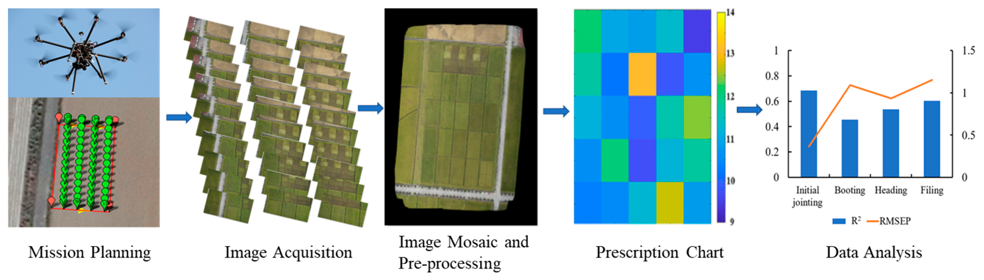
2. Materials and Methods

2.1. Image Acquisition

This study employs a combined approach of outdoor and indoor experiments to investigate the impact of varying flight parameters on image quality. The outdoor experiments were conducted in 2019 in Anhua Town, Zhuji City, Zhejiang Province, China (29°31′5.35″ N, 120°6′6.12″ E). The experimental area consisted of 100 plots, each measuring 9 × 5 m2, with a 1 m protection lane surrounding the plots. To acquire images of the rice crops, an octo-rotor UAV equipped with red–green–blue (RGB) and multispectral (MS) cameras was used. The UAV had a diameter of 1.1 m, a height of 0.35 m, and a maximum payload of 8 kg. The RGB camera used was the Sony A6000 micro single camera (Sony, Dugang District, Tokyo, Japan) equipped with a 16 mm fixed focus lens, and a resolution of 6000 pixels × 4000 pixels. The field of view of the lens is 83 degrees. The MS camera used was the MQ022MG-CM by XIMEA (Munster, Germany), equipped with a 16 mm fixed focus lens and a resolution of 409 pixels × 216 pixels. The field of view of the lens is 43.6 degrees. Throughout all experiments, manual exposure was employed, maintaining a consistent flight speed of 2.5 m/s, while setting the aperture of both cameras to 2.8. Further parameters regarding the RGB and MS cameras are detailed in Table 1.
Images were acquired under cloudless and windless weather conditions. The flight altitude varied between 15 m, 25 m, 30 m, 35 m, 40 m, 45 m, 50 m, 55 m, 100 m and 150 m, corresponding to ground sampling distances (GSDs) of 0.37 cm, 0.61 cm, 0.73 cm, 0.85 cm, 0.98 cm, 1.01 cm, 1.22 cm, 1.34 cm, 2.44 cm, and 3.65 cm for RGB cameras, respectively. Additionally, the GSDs of MS cameras were 2.58 cm, 4.29 cm, 5.16 cm, 6.02 cm, 6.88 cm, 7.74 cm, 8.59 cm, 9.46 cm, 17.18 cm, and 25.76 cm, respectively. Five images were taken at each flight altitude in the hovering state of the UAV. The same region of interest (ROI) was selected using MATLAB (2018a, 9.4.0.813654, MathWorks, Natick, Boulder, CO, USA) software and evaluated to represent the level of image quality at that altitude.
For a fixed altitude of 25 m, different combinations of exposure time and image overlap settings were explored. The flight speed of UAV is fixed at 2.5 m/s. The apertures of both cameras were set at 2.8. The exposure time of the RGB camera was set at two gradients: 1.25 ms and 1 ms. For the MS camera, exposure times were set at five gradients: 5, 6, 7, 16, and 20 ms. Due to the disparate field of view of the two cameras, the flight overlap was set based on the camera with the smaller field of view (MS). The designed gradients for the forward overlap were 65%, 75%, and 80%, while for the side overlap, three gradients of 55%, 60%, and 65% were employed. The specific experimental design of the flight parameter combinations is outlined in Table 2.
The MS images from the same flight mission were radiometrically calibrated and then stitched together to produce orthomosaic images using Agisoft Photoscan (Version 1.2.5, Agisoft LLC, St. Petersburg, Russia) software. This process involved the input of images and geographic coordinates, image alignment, mesh generation, texture generation, DEM creation and orthomosaic image generation. Geographic coordinates were acquired using GPS through a trigger signal on the UAV synchronized with the image. The mesh was computed based on the sparse point cloud due to the flat terrain. As the field of view of the RGB lens is greater than that of the MS, the acquired wide-angle images (RGB) were initially proportionally cropped to match the field of view of the MS images using MATLAB. Subsequently, these processed images were input into Agisoft Photoscan to obtain ortho-images following the same procedure. The MS and RGB ortho-images of the rice crops in the experimental field at a flight altitude of 25 m are shown in Figure 2.
To mitigate additional influences on image quality due to environmental factors such as surrounding wind speed and lighting changes during UAV flights, exposure time experiments were also conducted indoors. Using the same sensors as the UAV, the focal length and altitude were fixed to capture standardized reflectance gradient boards (with reflectance values of 12%, 25%, 50%, and 99%). For the RGB camera, exposure times were set at 24 gradients in a darkroom environment, ranging from 0.25 to 100 ms, corresponding to shutter speeds of 1/4000 to 1/10 s. The MS camera was set at 18 exposure time gradients ranging from 0.25 to 110 ms. It is worth noting that the aperture of both cameras remained constant during all experiments, both at 2.8.

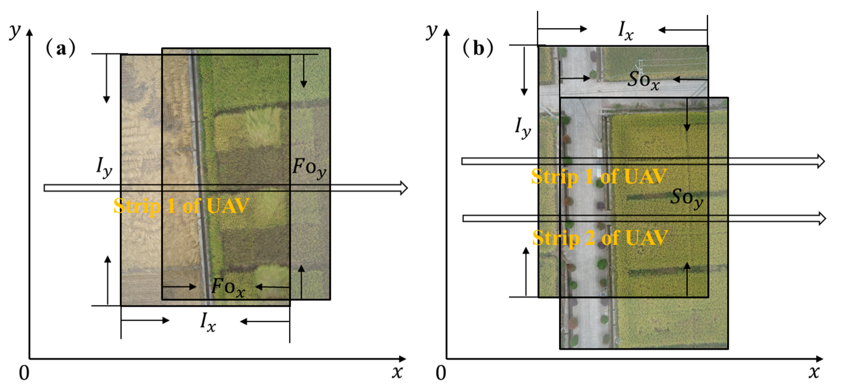
2.2. Overlap Calculation

During the UAV flight, the overlap between two adjacent images on the same flight strip is referred to as forward overlap (OF), while the overlap between two pictures on adjacent strips is known as side overlap (OS). There are generally two methods for calculating the degree of overlap. One is to represent the degree of OF and OS according to the length ratio of overlapping areas in different directions (Equations (1) and (2)). One is to represent the degree of image overlap according to the percentage of overlapping regions in the captured image area (Equations (3) and (4)). In this paper, Equation (3) is used as the standard of image overlap degree. Typically, an OF from 60% to 80% is required, with a minimum of 53%, while the OS should be at least 8%, with an optimal range from 15% to 60%. However, there is no consensus on how to select the overlap degree to obtain higher quality images. Figure 3 shows the schematic diagram of the overlap calculations method.
Based on the definition of overlap, OF and OS can be described as Equations (1) and (2). The formula for calculating the degree of image overlap based on the overlap area is shown in Equation (3).
O F = F o x I x × 100 %
O S = S o y I y × 100 %
O F = F o x × F o y I x × I y × 100 %
O S = S o x × S o y I x × I y × 100 %
where F o x and F o y represent the size of the overlap area in the flight direction. S o x and S o y represent the overlap of two pictures on two flight strips, and I x and I y indicates the size of the UAV image.

2.3. Image Evaluation

2.3.1. Conventional Image Quality Evaluation

Signal-to-noise ratio (SNR) is a commonly used metric to evaluate the noise level in an image. It measures the ratio of the signal strength to the noise level in the image. Higher SNR values indicate less noise and better image quality. This indicator is used to assess image quality when the exposure time is different and other conditions remain unchanged.
S N R = 10 L g P s P n ,
where P s is the power of the signal, P n is the power of the noise, and L g denotes the logarithm of the base 10.

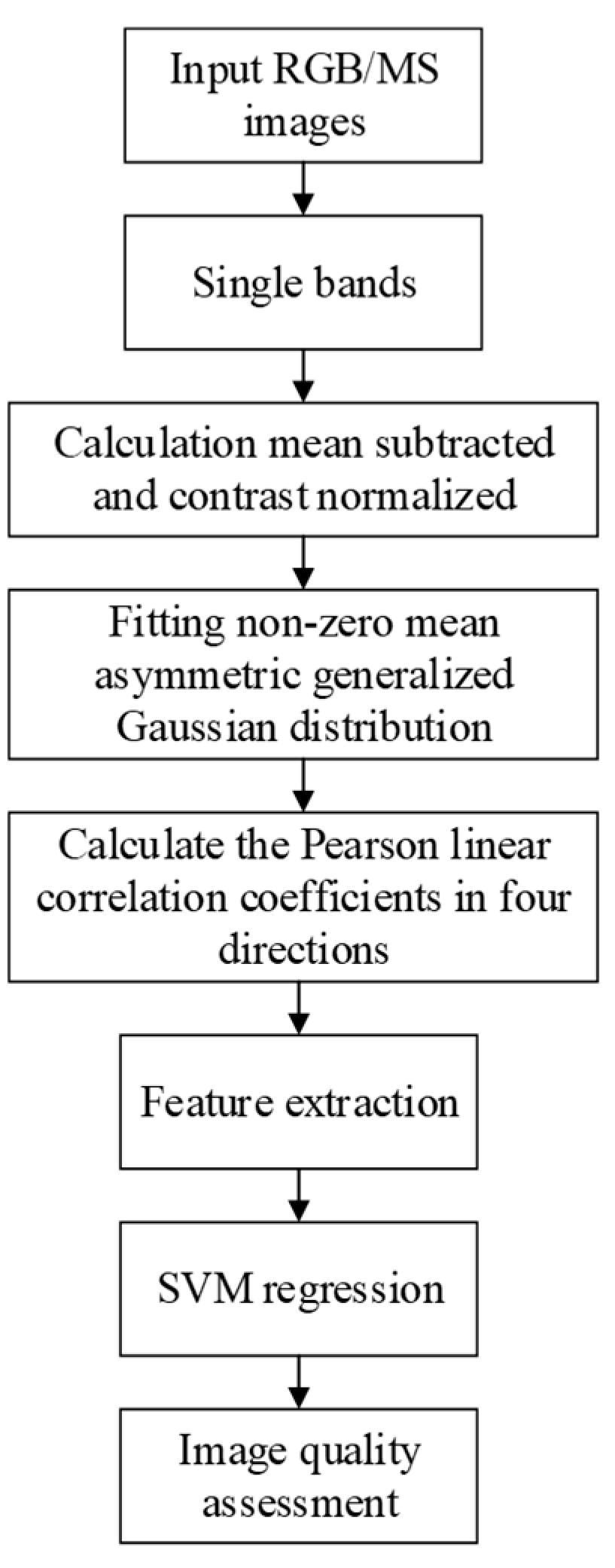
2.3.2. BRISQUE Algorithm

As remote sensing images lack original images for reference, a no-reference image quality assessment algorithm (NR-IQA) is selected to evaluate the quality of the obtained remote sensing images. Among the existing NR-IQA models for natural images, the Blind/Referenceless Image Spatial Quality Evaluator (BRISQUE) [10] is considered to be one of the most advanced and optimal models. BRISQUE not only considers image luminance [17], contrast [18], distortion [19], the complex statistic of an image [20], texture statistic [21], and Natural Scene Statistics (NSS) [22], but also maintains a relatively low computational complexity.
The algorithm can be summarized as follows. For a given (possibly distorted) image, locally normalized luminances are first computed via local mean subtraction and divisive normalization. Such an operation may be applied to a given intensity image I(i, j) to produce:
I ( i , j ) = I i , j μ ( i , j ) σ i , j + C ,
where, i ∈ 1, 2, …, M, j ∈ 1, 2, …, N are spatial indices; M and N are the image height and width, respectively; C = 1 is a constant that prevents instabilities from occurring when the denominator tends to zero and
σ ( i , j ) = w k . l ( I k . l i , j μ ( i , j ) 2 ) ,
μ ( i , j ) = w k . l I k . l ,
where w = { w k . l |   k = −K, …, K, l = −L, …, L} is a 2D circularly symmetric Gaussian weighting function sampled out to three standard deviations and rescaled to unit volume. In our implementation, K = L = 3. Meanwhile, the pre-processing model (6) is developed and refers to the transformed luminances I(i, j) as mean subtracted contrast normalized (MSCN) coefficients. Then, an asymmetric generalized Gaussian distribution (AGGD) can be used to effectively capture a broader spectrum of distorted image statistics. Additionally, Pearson linear correlation coefficients (PLCC) of MSCN adjacent coefficients in four directions of horizontal, vertical, main diagonal, and sub-diagonal are added to describe the characteristics of the overall structural distortion of the image. Finally, a support vector machine regression (SVM) [23] is used to learn from the feature space to quality scores, so it is worth noting that the better the image quality, the lower the score.
However, the algorithm only evaluates the quality of RGB images and is not applicable to MS images obtained using remote sensing. Notably, the research team adapted the BRISQUE algorithm to MS images by changing the image input to single band input and analyzing all bands to use the GGD fit of the MSCN coefficients. The average value of all bands is used as the quality evaluation score of the MS images. The algorithm flow chart is shown in Figure 4.

2.4. Methods for Removing Redundancy

The large amount of image data causes an increase in the time cost of the image stitching process. To solve this problem, a redundancy removal approach is proposed to streamline the UAV image data. The specific operation process of this method is shown in Figure 5. Step 1: input the UAV images with their respective BRISQUE scores. Step 2: Determine the redundancy interval, denoted as i, with a value range of integers greater than or equal to 0. The criterion for selection is the removal of redundancy to enable image mosaicking, as excessively low overlap between images can lead to mosaic failure. Step 3: Retain the image with the lowest quality score within the range of (i + 1) and remove the others. Then, proceed to the next redundancy interval. Step 4: repeat the above steps until all input images have been filtered. Step 5: Output all retained high-quality images. It is important to note that we need to perform image mosaicking on the retained images to obtain the final ortho-image. If the mosaicking process encounters difficulties, the redundancy interval should be reduced.

3. Results and Discussion

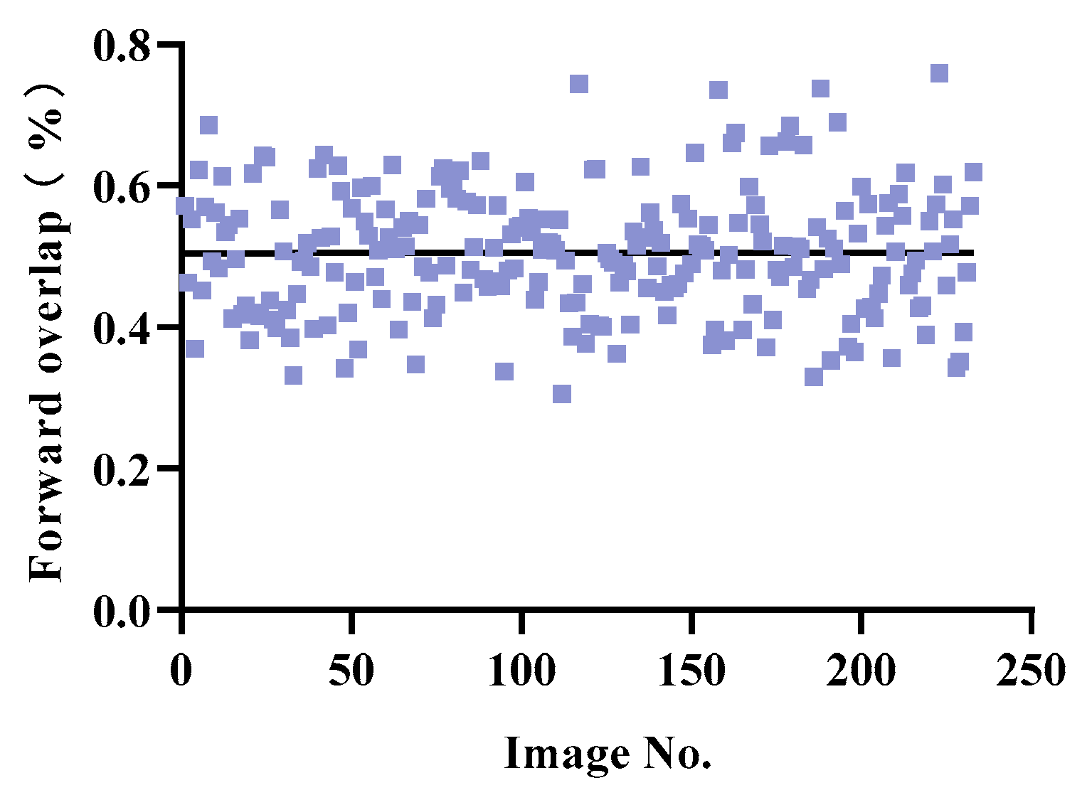
3.1. Calculation of Actual Overlap

Due to the complexity of the external environment, this study used the area method to calculate the actual overlap between two adjacent images, which is shown in Equation (3) in order to ensure the accuracy. According to the calculation method of overlap in the previous chapter, the data of all flights are analyzed. Taking the second experiment as an example, the results are illustrated in Figure 6. It can be observed that the overlap of the actual adjacent images acquired during the flight along the same strip fluctuates around a set value, rather than remaining at a fixed value. This fluctuation occurs due to the triggering signal method for UAV-controlled image capture being distance-based. Additionally, the autonomously developed UAV utilizes GPS for positioning, which may lead to positioning and drift errors during flight, resulting in this fluctuation phenomenon.
We also observed in Figure 6 that in Experiments 2 and 7, although the flight overlap was set at 80%, some actual values were below 60%. This is due to the fact that, given the determined UAV flight altitude and speed, increasing the image overlap requires shortening the capture interval. However, the exposure time during camera capture and the image storage time impose constraints on the capture interval. When the capture interval cannot meet the image storage requirements, some images may be missed. Therefore, in the scenario of a UAV flying at a speed of 2.5 m per second and at a flight altitude of 25 m, it is recommended to set the OF to not exceed 75% to ensure data integrity. When a higher flight speed is attainable, adjusting the flight altitude to maintain the capture interval in accordance with image acquisition requirements is feasible. Alternatively, a lower altitude can be employed in conjunction with reduced flight speed. Substituting the imaging sensor with a faster storage speed can also fulfill the demand for increased image overlap.

3.2. UAV Image Quality Evaluation

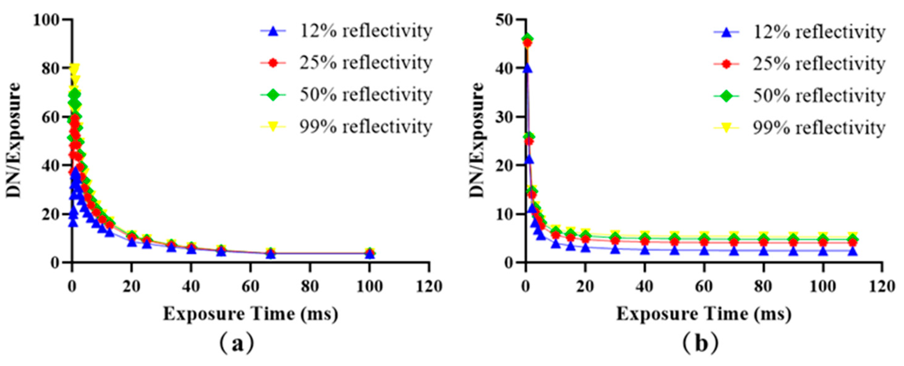
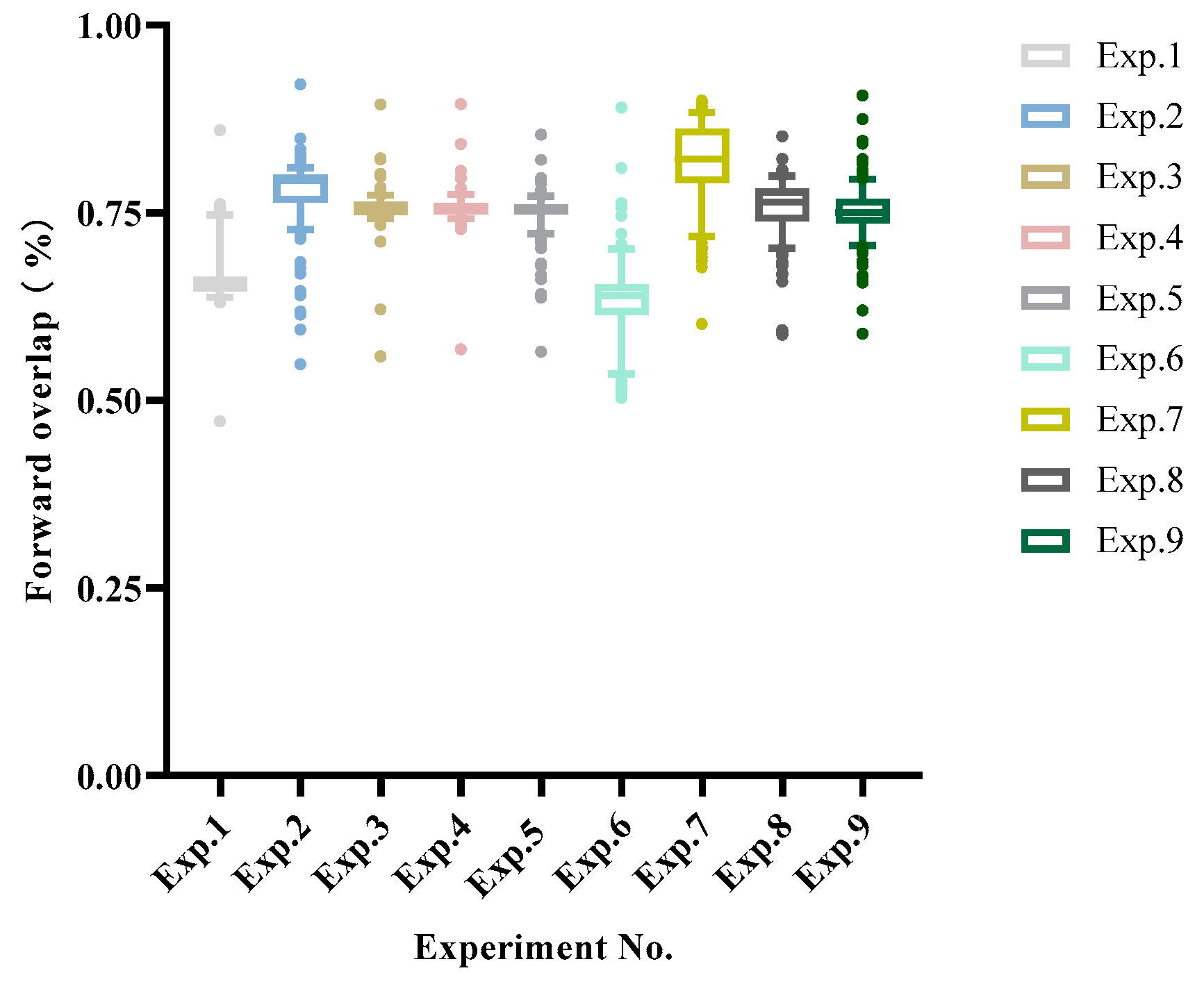
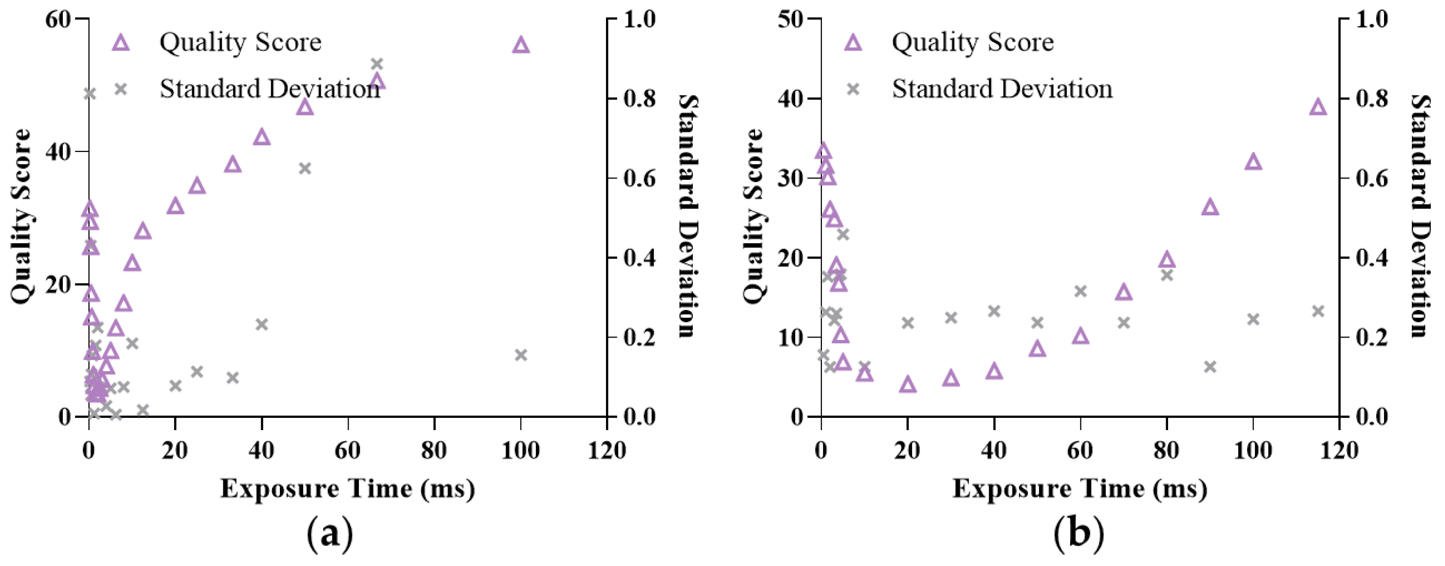
3.2.1. Influence of Exposure Time on Image Quality Evaluation

The linearity of the ratio of DN to exposure time for the four reflectivity targets is demonstrated in Figure 7. Notably, as the exposure time increases, the linearity of the targets becomes more stable. This observation holds true even when keeping the light intensity, camera height, and focal length constant.
Figure 8 depicts the SNR values obtained for different exposure times and three different types of reflection. It can be observed that the image SNR values increase as the exposure time increases. However, the SNR values reach a plateau after a certain level due to the saturation of image DNs. The maximum SNR levels for different channels are dependent on the dark noise level of each channel. In practical scenarios, it is recommended to select integration time settings that optimize image SNRs while avoiding image saturation. For instance, in low irradiance conditions and low reflectivity land covers, the optimal integration time coincides with the maximum integration time. On the other hand, for high-reflectivity targets, exposure times with better linearity and lower sensitivity should be chosen.
In the presence of constant light intensity, the relationship between the image quality score and exposure time for both the RGB and MS cameras is illustrated in Figure 9. Evidently, the image quality scores obtained by both cameras exhibit a trend of initially decreasing and then increasing with longer exposure times. Notably, the RGB camera is capable of achieving a higher image quality (QS < 10) between 0.8 ms and 5 ms, whereas the MS images demonstrate this between 4 ms and 50 ms.
In the outdoor environment, the BRISQUE algorithm is used to evaluate the image quality of five different exposure time setting experiments of MS camera. The probability analysis of five flights is shown in Figure 10. We can find that the probability distribution of image quality is different under different exposure time settings. Overall, during a single UAV flight experiment, fluctuations in external environmental conditions lead to variations in the quality of image acquisition.

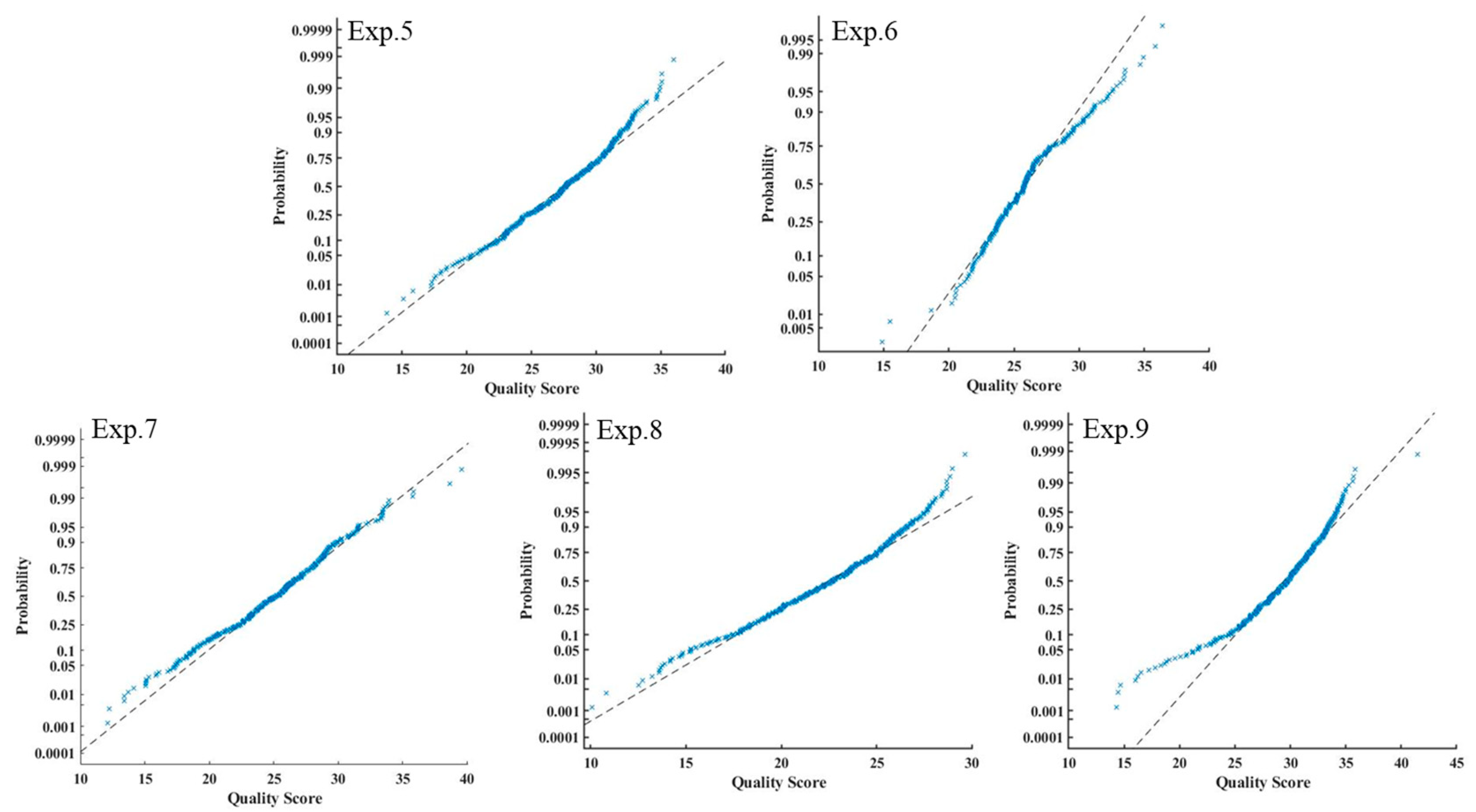
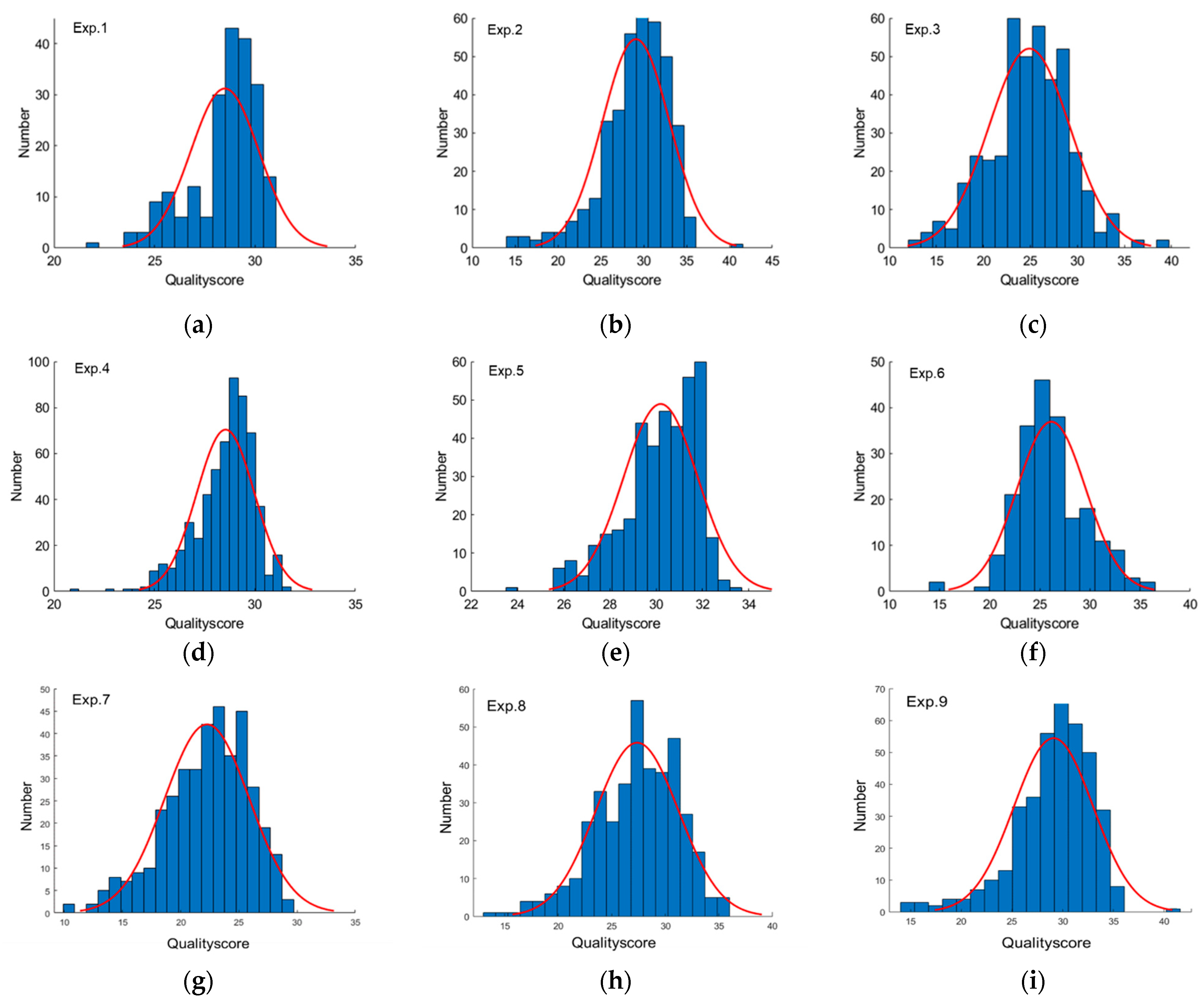
3.2.2. Image Quality Evaluation of Single Experiment

In this paper, the improved BRISQUE algorithm is used to evaluate the image quality of MS images and RGB images obtained using a UAV. The quality score is shown in Figure 11. The lower the score that we calculated, the better the required image quality since support vector machine regression is used in this algorithm. It can be seen from the figure that the quality score of remote sensing images in the same experience is in the form of a normal distribution. The position of the expected value depends on the matching degree between the exposure time set by the experimenter at takeoff and the light intensity at that time. In the process of UAV operation, due to the change in illumination intensity, the image quality obtained in one experiment is not invariable. Therefore, we can try to explore whether removing lower-quality remote sensing images can obtain higher-quality mosaic images. The setting of high overlap makes it possible to reduce image redundancy.

3.2.3. Image Quality Evaluation of Different Flight Altitude

The UAV flies at different altitudes to obtain five crop RGB and MS remote sensing images. The obtained image quality is evaluated using the BRISQUE algorithm. The box chart (Figure 12) shows the image quality scores at different altitudes (15 m, 25 m, 30 m, 35 m, 40 m, 45 m, 50 m, 100 m, 150 m). Comparing the average scores of different altitudes, we can find that the image quality scores of RGB images obtained between 15 m and 150 m show a fluctuating increase, but there is a large difference at the same altitude. This is because the factors affecting the image quality score at lower flight altitudes depend more on the suitability between the variation in light intensity and the exposure time setting.
The MS image quality score exhibits a trend of decreasing and then increasing, with an average optimal score achieved at a flight altitude of 30 m. In general, higher flight altitudes lead to lower image quality. The higher image quality at 30 m may be attributed to the camera acquiring more crop information under relatively stable external environmental conditions, thereby improving the quality score to a certain extent. However, due to the low resolution of the MS camera, exceeding a certain flight altitude results in a low ground resolution that erases surface texture information, ultimately affecting the comprehensive score. Therefore, when using the two cameras described in this paper to obtain remote sensing images of crops, it is recommended to maintain a flight altitude between 15 and 35 m.

3.3. Image Mosaic and Redundancy Reduction

Initially, all images based on the same flight were input into the software to obtain an orthomosaic image, and the time from the image input to final ortho-image was recorded. A fixed redundancy interval was selected based on the OF, and the images were stitched again. This process was repeated until stitching failed. The number of images and splicing time of the last successful splicing were recorded as the final result of redundant processing. The image quality of the acquired ortho-images was evaluated using the BRISQUE algorithm.
Figure 13 illustrates the variation in image overlap after three rounds of redundancy removal in the second experiment, decreasing from the original 80% to fluctuate at around 45%. As the decrease in overlap makes image mosaicking challenging, the images after three rounds of redundancy removal cannot be stitched to obtain ortho-images. Therefore, the final retained high-quality images are those processed for redundancy twice. According to the results, it is recommended that during the flight, the forward overlap factor should reach at least 60% to ensure a proper image alignment. However, considering the inherent errors associated with the use of consumer-grade small-format digital cameras (such as the SONY camera we utilized) in small UAV photogrammetry, as well as the importance of larger overlaps in mitigating variations due to slight topographic height differences and enhancing the overall robustness of the image block adjustments, the setting of overlap parameters can be increased as much as possible while ensuring complete image coverage.
Figure 14 illustrates changes in the number of images and mosaic image quality scores before and after redundancy removal in all experiments. Additionally, Table 3 displays the completion time of obtaining the mosaic image. The image mosaic efficiency and the mosaic image quality of experiments were improved to varying degrees after reducing redundancy, except in the case of Experiment 6. Fortunately, the maximum improvement in image stitching efficiency was 84% (Experiment 7), while the image quality score improved by 7%. Meanwhile, Experiment 2, with the largest improvement in image quality scores (13%), had a 30% reduction in completion time. The reason for the absence of redundancy reduction in Experiment 6 was that the resolution of the MS camera is lower than that of RGB, and there are fewer feature points in the process of image stitching, which makes the stitching more difficult. In addition, the overlap is too low after redundancy reduction, which leads to stitching failure. Therefore, it is not necessary to reduce the redundancy of low-overlap MS images. The higher the overlap degree is set, the more images of the target area are obtained, and the larger the amount of redundancy data. Therefore, for a large number of images obtained using a high overlap, image redundancy reduction can not only improve the efficiency of image mosaicking, but also improve the quality of image stitching to a certain extent. Simultaneously, it is possible to appropriately increase the fixed redundancy interval based on the overlap to enhance image processing efficiency.

4. Discussion of Flight Strategy

When considering the utilization of UAVs for image acquisition, a comprehensive assessment of various factors such as flight altitude, exposure time, flight speed, and flight overlap is essential to obtain comprehensive crop information. It is important to note that the configuration of these parameters directly impacts the quality and efficiency of image acquisition, and their interrelationships play a crucial role in devising effective flight strategies. In the realm of camera optics, to obtain clear images without causing motion blur during the process of capturing dynamic images, the exposure time and flight speed must satisfy the condition outlined in Equation (9). The calculation of GSD is directly related to the flight altitude (Equation (10)). As a result, the interplay between flight altitude, flight speed, and exposure time is elucidated through the relationships depicted in Equation (9) and Equation (10). It is noteworthy that the configuration of flight speed primarily influences the capture of clear images. When GSD remains constant, setting the exposure time requires careful consideration of factors such as camera performance, solar radiation intensity, and white balance, thereby adding complexity to the decision-making process. These factors directly impact the imaging quality of the acquired images, underscoring the importance of prioritizing exposure time requirements when formulating flight strategies. In contrast, considerations for flight speed are relatively straightforward once exposure time requirements are met. Consequently, this study focuses on exploring methods for setting exposure time, while maintaining a consistent flight speed.
E T × V G S D ,
G S D = S × H f ,
where E T is exposure time, V is flight speed, G S D is ground sample distance, S is camera single pixel size, H is flight altitude above ground, and f is focal length.
By utilizing this formula, the longest exposure times required during UAV-mounted camera flights can be determined. Consequently, in this study, under the conditions of a flight speed of 2.5 m/s and a flight altitude of 25 m, the respective maximum exposure times for the RGB and MS cameras are within 1.1 ms and 16 ms. Figure 7, Figure 8, Figure 9 and Figure 10 demonstrate that exposure time directly influences image quality, with shorter exposure times resulting in lower signal-to-noise ratios. The results indicate that maintaining the exposure time for the RGB camera between 0.8 ms and 5 ms, as well as selecting an exposure time between 4 ms and 50 ms for the MS camera, contributes to achieving higher signal-to-noise ratios and better image quality. Therefore, considering the aforementioned requirements, the exposure time for the RGB camera should be set between 0.8 ms and 1.1 ms, and for the MS camera, it should be set between 4 and 16 ms. Furthermore, adjustments to aperture and ISO can maintain a consistent white balance in the images, even amidst changes in external environmental conditions.
The setting of the UAV’s flight forward overlap is closely related to the field of view of the mounted camera, as expressed by Equation (5).
O F = 2 × H × t a n ( θ 2 ) V ,
where O F is forward overlap, H is flight altitude, V is flight speed, θ is field of view of lens along the short frame side.
This indicates that the forward overlap is inversely proportional to the flight speed and directly proportional to the flight height and the camera’s field of view, as demonstrated by Equation (11). A higher OF can be achieved by reducing the flight speed, increasing the flight altitude, or employing a camera with a larger field of view while maintaining a consistent shooting interval. Figure 12 confirms that the appropriate GSD leads to a high image quality, with an optimal image quality obtained within the flight altitude range of 15–35 m. Therefore, priority should be given to reducing the flight speed or adjusting the camera’s field of view to enhance the overlap. Additionally, under constant flight altitude, speed, and camera specifications, increasing the overlap can also be achieved by reducing the photo capture interval. However, this method requires consideration of the camera’s exposure time, as outlined in the aforementioned Equation (9).
In the post-data collection processing and analysis workflow, greater emphasis is placed on the quality and efficiency of image stitching. Figure 11 demonstrates the uneven quality of images captured during the same flight mission. Figure 14 illustrates that by selecting high-quality images and reducing redundancy, not only can the efficiency of image stitching be improved, but the stitching quality can also be enhanced. Therefore, during UAV image acquisition, setting a higher overlap can contribute to obtaining higher-quality stitched images, while ensuring exposure time.
Based on the above analysis, when using both RGB and MS cameras for crop image acquisition in this study, it is recommended to maintain a flight altitude of between 15 and 35 m. Furthermore, it is recommended to set the exposure time for the RGB camera between 0.8 ms and 1.1 ms, and for the MS camera within the range of 4–16 ms, when both camera apertures are set to 2.8. This approach is more likely to yield higher-quality images. Regarding the flight OF, a value of approximately 75% is suggested, as it adequately meets the requirements for both flight altitude and exposure time. Certainly, it is possible to increase the overlap while ensuring the complete acquisition of images.
In addition, UAV flight parameters should be varied accordingly for different terrains [24]. This is because factors such as different terrain types, elevation, vegetation density and reflective surfaces have a significant impact on the planning and execution of UAV survey or mapping missions. For instance, areas with tall vegetation may introduce shadows and varying light levels, mandating careful adjustments to exposure settings to ensure optimal image quality. Similarly, snow-covered areas, water bodies, and urban environments may require exposure adjustments to prevent over- or underexposure. Moreover, higher elevations may demand adjustments to the flight altitude to maintain the desired GSD and uphold image quality, while complex terrains, such as mountainous regions or areas with significant elevation changes, may require a higher overlap between images to capture comprehensive data effectively. Additionally, dense vegetation can obstruct the view of the ground, potentially requiring a higher overlap to capture sufficient data for accurate image stitching and subsequent analysis. Considering these aspects enhances the robustness of the image acquisition strategy, ensuring that the set parameters align with the specific characteristics of the UAV-mapped area and thereby contribute to the acquisition of high-quality and comprehensive image data for subsequent analysis.

5. Conclusions

In this study, we achieved UAV flight parameter optimization and obtained high-quality stitched images by investigating the effects of different exposure times, flight altitudes, and OF settings on the image quality of rice phenology. We used an eight-rotor UAV flight platform equipped with two image acquisition sensors, including MS and RGB cameras, to capture images of rice crops. The experimental design included a combination of three different variables such as exposure time, flight altitude and overlap. All experimental flights were conducted at the same speed. The SNR was used to evaluate the noise level of the images, and an improved BRISQUE algorithm was proposed to assess the quality of the MS and RGB remote sensing images. The results indicate that exposure time directly influences the quality of low-altitude remote sensing images obtained by UAVs, with shorter exposure times leading to lower signal-to-noise ratios. Additionally, obtaining clear images during UAV motion requires specific conditions. Based on our study, when both camera apertures are set to 2.8, the optimal exposure time for the RGB camera should be between 0.8 ms and 1.1 ms, and for the MS camera, the exposure time should range between 4 and 16 ms. Based on these experiments, it is recommended to capture images at flight altitudes between 15 m and 35 m. Meanwhile, the OF setting of the UAV needs to take into account the flight altitude and exposure time, and a high OF will lead to image loss. Therefore, choosing the appropriate OF is crucial for image acquisition, and the results of this study show that a flight OF of about 75% can satisfy the needs of image acquisition. Finally, in the subsequent image processing stage, a method for removing image redundancy proposed in this study can effectively improve the quality (13%) and efficiency (84%) of image stitching, which provides an idea for the effective utilization of data and reduction in time cost.

6. Patents

The US invention patents resulting from the work reported in this manuscript have been authorized—patent number: US 11636582B1.

Author Contributions

Conceptualization, Methodology, Software, Formal Analysis, X.D.; Investigation, X.D. and L.Z.; Data Curation, X.D., L.Z. and J.Z.; Writing—Original Draft Preparation, X.D.; Methodology, Writing—Review and Editing, H.C.; Writing—Review and Editing, Funding Acquisition, Y.H. All authors have read and agreed to the published version of the manuscript.

Funding

This research was funded by Key R & D projects in Zhejiang Province, grant number 2021C02023.

Data Availability Statement

All data used to support the findings of this study are included within the article.

Conflicts of Interest

The authors declare no conflicts of interest.

References

  1. Lan, Y.; Thomson, S.J.; Huang, Y.; Hoffmann, W.C.; Zhang, H. Current Status and Future Directions of Precision Aerial Application for Site-Specific Crop Management in the USA. Comput. Electron. Agric. 2010, 74, 34–38. [Google Scholar] [CrossRef]
  2. Lu, W.; Okayama, T.; Komatsuzaki, M. Rice Height Monitoring between Different Estimation Models Using UAV Photogrammetry and Multispectral Technology. Remote Sens. 2022, 14, 78. [Google Scholar] [CrossRef]
  3. Yue, J.; Yang, G.; Tian, Q.; Feng, H.; Xu, K.; Zhou, C. Estimate of Winter-Wheat above-Ground Biomass Based on UAV Ultrahigh-Ground-Resolution Image Textures and Vegetation Indices. ISPRS J. Photogramm. Remote Sens. 2019, 150, 226–244. [Google Scholar] [CrossRef]
  4. Zhang, X.; Zhang, K.; Wu, S.; Shi, H.; Sun, Y.; Zhao, Y.; Fu, E.; Chen, S.; Bian, C.; Ban, W. An Investigation of Winter Wheat Leaf Area Index Fitting Model Using Spectral and Canopy Height Model Data from Unmanned Aerial Vehicle Imagery. Remote Sens. 2022, 14, 5087. [Google Scholar] [CrossRef]
  5. Ma, Y.; Zhang, Q.; Yi, X.; Ma, L.; Zhang, L.; Huang, C.; Zhang, Z.; Lv, X. Estimation of Cotton Leaf Area Index (LAI) Based on Spectral Transformation and Vegetation Index. Remote Sens. 2021, 14, 136. [Google Scholar] [CrossRef]
  6. Xu, X.Q.; Lu, J.S.; Zhang, N.; Yang, T.C.; He, J.Y.; Yao, X.; Cheng, T.; Zhu, Y.; Cao, W.X.; Tian, Y.C. Inversion of Rice Canopy Chlorophyll Content and Leaf Area Index Based on Coupling of Radiative Transfer and Bayesian Network Models. ISPRS J. Photogramm. Remote Sens. 2019, 150, 185–196. [Google Scholar] [CrossRef]
  7. Kefauver, S.C.; Vicente, R.; Vergara-Díaz, O.; Fernandez-Gallego, J.A.; Kerfal, S.; Lopez, A.; Melichar, J.P.E.; Serret Molins, M.D.; Araus, J.L. Comparative UAV and Field Phenotyping to Assess Yield and Nitrogen Use Efficiency in Hybrid and Conventional Barley. Front. Plant Sci. 2017, 8, 1733. [Google Scholar] [CrossRef] [PubMed]
  8. Wan, L.; Cen, H.; Zhu, J.; Zhang, J.; Zhu, Y.; Sun, D.; Du, X.; Zhai, L.; Weng, H.; Li, Y.; et al. Grain Yield Prediction of Rice Using Multi-Temporal UAV-Based RGB and Multispectral Images and Model Transfer—A Case Study of Small Farmlands in the South of China. Agric. For. Meteorol. 2020, 291, 108096. [Google Scholar] [CrossRef]
  9. Fu, Z.; Jiang, J.; Gao, Y.; Krienke, B.; Wang, M.; Zhong, K.; Cao, Q.; Tian, Y.; Zhu, Y.; Cao, W.; et al. Wheat Growth Monitoring and Yield Estimation Based on Multi-Rotor Unmanned Aerial Vehicle. Remote Sens. 2020, 12, 508. [Google Scholar] [CrossRef]
  10. Liu, Y.; An, L.; Wang, N.; Tang, W.; Liu, M.; Liu, G.; Sun, H.; Li, M.; Ma, Y. Leaf Area Index Estimation under Wheat Powdery Mildew Stress by Integrating UAV-based Spectral, Textural and Structural Features. Comput. Electron. Agric. 2023, 213, 108169. [Google Scholar] [CrossRef]
  11. Torres-Sánchez, J.; Peña-Barragán, J.M.; Gómez-Candón, D.; De Castro, A.I.; López-Granados, F. Imagery from Unmanned Aerial Vehicles for Early Site Specific Weed Management. In Proceedings of the Precision Agriculture, Lleida, Spain, 7–11 July 2013; pp. 193–199. [Google Scholar]
  12. Faiçal, B.S.; Freitas, H.; Gomes, P.H.; Mano, L.Y.; Pessin, G.; de Carvalho, A.C.P.L.F.; Krishnamachari, B.; Ueyama, J. An Adaptive Approach for UAV-Based Pesticide Spraying in Dynamic Environments. Comput. Electron. Agric. 2017, 138, 210–223. [Google Scholar] [CrossRef]
  13. Song, C.; Liu, L.; Wang, G.; Han, J.; Zhang, T.; Lan, Y. Particle Deposition Distribution of Multi-Rotor UAV-Based Fertilizer Spreader under Different Height and Speed Parameters. Drones 2023, 7, 425. [Google Scholar] [CrossRef]
  14. Gu, J.; Zhang, R.; Dai, X.; Han, X.; Lan, Y.; Kong, F. Research on Setting Method of UAV Flight Parameters Based on SLAM. J. Chin. Agric. Mech. 2022, 43, 2095–5553. [Google Scholar]
  15. Hu, S.; Cao, X.; Deng, Y.; Lai, Q.; Wang, G.; Hu, D.; Zhang, L.; Liu, M.; Chen, X.; Xiao, B.; et al. Effects of the Flight Parameters of Plant Protection Drone on the Distribution of Pollination Droplets and the Fruit Setting Rate of Camellia. Trans. Chin. Soc. Agric. Eng. (Trans. CSAE) 2023, 39, 92–100. [Google Scholar] [CrossRef]
  16. He, Y.; Du, X.; Zheng, L.; Zhu, J.; Cen, H.; Xu, L. Effects of UAV Flight Height on Estimated Fractional Vegetation Cover and Vegetation Index. Trans. Chin. Soc. Agric. Eng. (Trans. CSAE) 2022, 38, 63–72. [Google Scholar]
  17. Mittal, A.; Moorthy, A.K.; Bovik, A.C. No-Reference Image Quality Assessment in the Spatial Domain. IEEE Trans. Image Process. 2012, 21, 4695–4708. [Google Scholar] [CrossRef] [PubMed]
  18. Fang, Y.; Ma, K.; Wang, Z.; Lin, W.; Fang, Z.; Zhai, G. No-Reference Quality Assessment of Contrast-Distorted Images Based on Natural Scene Statistics. IEEE Signal Process. Lett. 2015, 22, 838–842. [Google Scholar] [CrossRef]
  19. Moorthy, A.K.; Bovik, A.C. Blind Image Quality Assessment: From Natural Scene Statistics to Perceptual Quality. IEEE Trans. Image Process. 2011, 20, 3350–3364. [Google Scholar] [CrossRef]
  20. Ye, P.; Doermann, D. No-Reference Image Quality Assessment Using Visual Codebooks. IEEE Trans. Image Process. 2012, 21, 3129–3181. [Google Scholar] [CrossRef]
  21. Tang, H.; Joshi, N.; Kapoor, A. Learning a Blind Measure of Perceptual Image Quality. In Proceedings of the IEEE Computer Society Conference on Computer Vision and Pattern Recognition, Colorado Springs, CO, USA, 20–25 June 2011; pp. 305–312. [Google Scholar]
  22. Saad, M.A.; Bovik, A.C.; Charrier, C. Blind Image Quality Assessment: A Natural Scene Statistics Approach in the DCT Domain. IEEE Trans. Image Process. 2012, 21, 3339–3352. [Google Scholar] [CrossRef]
  23. Schölkopf, B.; Smola, A.J.; Williamson, R.C.; Bartlett, P.L. New Support Vector Algorithms. Neural Comput. 2000, 12, 1207–1245. [Google Scholar] [CrossRef] [PubMed]
  24. Storch, M.; Jarmer, T.; Adam, M.; de Lange, N. Systematic Approach for Remote Sensing of Historical Conflict Landscapes with UAV-Based Laserscanning. Sensors 2022, 22, 217. [Google Scholar] [CrossRef] [PubMed]
Figure 1. Flow chart from image acquisition to data analysis based on UAV.
Drones 08 00143 g001
Figure 2. Ortho-images of multispectral camera (a) and RGB camera (b) at a flight altitude of 25 m.
Drones 08 00143 g002
Figure 3. Diagram of the degree of image forward overlap (a) and side overlap (b).
Drones 08 00143 g003
Figure 4. Algorithm flow chart of the improved BRISQUE algorithm.
Drones 08 00143 g004
Figure 5. Image selection method for removing redundancy.
Drones 08 00143 g005
Figure 6. Forward overlap (OF) of all experiments.
Drones 08 00143 g006
Figure 7. Ratio of digital number (DN) to exposure time for four reflectivity targets with an RGB camera (a) and MS camera (b).
Drones 08 00143 g007
Figure 8. Signal-to-noise ratio (SNR) for different exposure time settings and targets with an MS camera: (a) 12% reflectivity, (b) 50% reflectivity, and (c) 99% reflectivity under constant illumination. The x-axis represents the different channels, and the y-axis is the image SNR.
Drones 08 00143 g008
Figure 9. Relationship between quality score (QS) and exposure time with an RGB camera (a) and MS camera (b).
Drones 08 00143 g009
Figure 10. Probability analysis of quality evaluation distribution of five flights with an MS camera.
Drones 08 00143 g010
Figure 11. Quality evaluation distribution of nine flight experiments (ai) based on the BRISQUE algorithm.
Drones 08 00143 g011
Figure 12. Quality evaluation of different flight altitudes based on BRISQUE algorithm with RGB camera (a) and MS camera (b).
Drones 08 00143 g012
Figure 13. Forward overlap (OF) of the second experiment after two redundancy removals.
Drones 08 00143 g013
Figure 14. The changes in the number of images (a) and quality evaluation of the mosaic image (b) before and after the removal redundancy in each flight experiment.
Drones 08 00143 g014
Table 1. Parameters of RGB and MS cameras.
CameraName Parameter
RGBWeight 358 g
Sensor size23.4 mm × 15.6 mm
Resolution 6000 pixels × 4000 pixels
Focus lens16 mm/fixed
Field of view 83
MSWeight 123 g
Sensor size11.27 mm × 6 mm
Resolution 409 pixels × 216 pixels
Focus lens16 mm/fixed
Field of view 43.6
Bands 600–1000 nm
Note: The field of view is calculated diagonally.
Table 2. Summary of flight campaigns and parameter settings at a flight altitude of 25 m.
CameraExperimentsExposure Time (ms)Forward
Overlap (%)
Side Overlap (%)Number of Images
RGBExp. 116555221
Exp. 218065577
Exp. 317560387
Exp. 41.257560388
MSExp. 557560387
Exp. 666555211
Exp. 778065577
Exp. 8167560387
Exp. 9207560388
Table 3. Quality evaluation of mosaic image before and after redundancy reduction.
CameraExperimentsCompletion Time (h)
BeforeAfterImproved
RGBExp. 11.020.7526%
Exp. 22.161.530%
Exp. 32.41.7527%
Exp. 419.41048%
MSExp. 50.080.0713%
Exp. 60.050.050
Exp. 70.50.0884%
Exp. 80.090.0811%
Exp. 90.090.0811%
Disclaimer/Publisher’s Note: The statements, opinions and data contained in all publications are solely those of the individual author(s) and contributor(s) and not of MDPI and/or the editor(s). MDPI and/or the editor(s) disclaim responsibility for any injury to people or property resulting from any ideas, methods, instructions or products referred to in the content.

