A Dynamic Visual SLAM System Incorporating Object Tracking for UAVs

Abstract

The capability of unmanned aerial vehicles (UAVs) to capture and utilize dynamic object information assumes critical significance for decision making and scene understanding. This paper presents a method for UAV relative positioning and target tracking based on a visual simultaneousocalization and mapping (SLAM) framework. By integrating an object detection neural network into the SLAM framework, this method can detect moving objects and effectively reconstruct the 3D map of the environment from image sequences. For multiple object tracking tasks, we combine the region matching of semantic detection boxes and the point matching of the optical flow method to perform dynamic object association. This joint association strategy can prevent trackingoss due to the small proportion of the object in the whole image sequence. To address the problem ofacking scale information in the visual SLAM system, we recover the altitude data based on a RANSAC-based plane estimation approach. The proposed method is tested on both the self-created UAV dataset and the KITTI dataset to evaluate its performance. The results demonstrate the robustness and effectiveness of the solution in facilitating UAV flights.

1. Introduction

Unmanned aerial vehicles (UAVs) have been used in diverse domains, such asogistics, rescue operations, and wildlife protection. Enhancing the visual perception capabilities of UAVs is essential for robust navigation in some challenging flight scenarios. The UAVs equipped with cameras can capture images of surroundings, which provide motion cues for trajectory estimation and 3D mapping. This visual perception approach primarily relies on the utilization of simultaneousocalization and mapping (SLAM) or visual odometry (VO) technologies [1]. While there are various visual SLAM frameworks available [2,3,4,5,6], their direct application to UAV navigation applications often overlooks the presence of dynamic objects within the environment. Thisimitation hampers their applicability in real-world scenarios, where the detection, tracking, and mapping of dynamic objects are crucial for the safety of UAVs [7]. Therefore, there is a need for specialized algorithms that can effectively handle dynamic objects in visual SLAM systems for UAVs.

Over the past decade, significant attention has been devoted to addressing the challenge of handling dynamic objects in SLAM algorithms. Traditional approaches employ two main strategies: (1) detecting moving regions within the scene and disregarding these regions [8,9,10,11]; (2) synthesizing plausible color, texture, and geometry in regions occluded by dynamic objects during image stream processing [12,13]. Both strategies result in the exclusion of information about dynamic objects, leading to the generation of static-only maps. Most recently, certain researchers have adopted a different perspective by integrating dynamic object tracking into the SLAM problem [14]. By taking into account the dynamics of moving objects, these approaches strive to go beyond static mapping andocalization, aiming to improve the overall understanding of the environment.

Despite the numerous efforts aimed to enhance the capabilities of visual SLAM by incorporating the detection and tracking of dynamic objects, there is still a significant gap in the field of UAV navigation. A common problem is that the UAV-borne monocular camera oftenacks the ability to restore real scale information, making it challenging to estimate the actual speed of dynamic objects. In addition, objects captured in UAV-borne images often exhibit sparsity and uneven distribution, which consequently increases the probability of missed detections. In this paper, we present a monocular visual SLAM algorithm explicitly designed for UAVs, which aims to achieve efficient 3D mapping and target tracking and positioning. The scale recovery method enables converting the semantic detection results into meaningful geometric motion results of objects, which can provide target motion parameters with actual physical quantities. Our work was inspired by the VDO-SLAM method. However, one innovation is its ability to estimate object motion models for UAV-borne images, and the proposed method can obtain motion parameters of the targets with real physical scale, which cannot be solved by VDO-SLAM or ORB-SLAM2.

Indeed, we proposed two innovations:

(a)

Combining object-wise matching and point-wise matching to track dynamic objects. It solves the problem of tracking instability caused by small target pixel regions and is of great significance for airborne observation systems.

(b)

A new trained network model for UAV datasets. It should be noted that the application scenarios of UAVs are different from traditional vehicle scenarios, and simple combinations cannot fully solve such problems. So, we trained a network model suitable for UAV datasets and achieved success through experimental testing.

The proposed SLAM algorithmeverages the random sample consensus (RANSAC) method [15] to estimate and restore scale information by fitting a ground plane. Both object-wise matching and point-wise matching are employed within the algorithm to achieve joint tracking of dynamic objects. Object-wise matching enables efficient and rapid tracking of dynamic objects, while point-wise matching addresses missed detections from the object detection network. Consequently, the final map constructed encompasses both dynamic objects and static environments.

This paper is organized into the following sections. Next, Section 2 provides a comprehensive review of related work in this field. Section 3 outlines the methodology employed in our study. The experimental setup is presented in Section 4, followed by the results and evaluations. Finally, Section 5 summarizes and presents concluding remarks.

2. Related Work

The visual SLAM algorithms applied to UAV flight include several steps, covering a range of research topics. To provide a thorough understanding of the background, we present a review of theiterature in Section 2.1 and Section 2.2, covering visual SLAM and dynamic object tracking, respectively. Furthermore, in Section 2.3, we discuss the existing technologies for UAV systems.

2.1. Dynamic Visual SLAM

Early pioneering approaches in visual SLAM are mainly pure feature-based methods. They relied on extracting and matching distinctive features in the images to estimate the cameras’ poses relative to the world coordinate system, such as MonoSLAM [16], PTAM [17], ORB-SLAM [4], and ORB-SLAM2 [6]. Inheriting the framework of ORB-SLAM2, subsequent SLAM systems commonly comprise three distinct threads: (1) a tracking thread, responsible for tracking point-wise features (i.e., ORB features [18]) and estimating poses; (2) a mapping thread, which constructs aocal 3D map and eliminates redundant keyframes; and (3) aoop closing thread, which corrects the accumulated drift and performs global optimization. This design enables the algorithms to operate continuously for extended periods inarge-scale scenes with significantoops, ensuring global consistency of the trajectory and the map. Benefiting from the efficiency of this design, many new methodologies [10,11,19,20,21,22] are integrated and tested on the widely used ORB-SLAM2 frameworks. The selection of keyframes is important to the system’s performance by maintaining good accuracy and robustness [23]. The understanding of dynamic scenes is generally based on keyframes. In many applications, prior knowledge is of great significance for understanding dynamic scenes. However, unlike someiDAR-based SLAM systems [24,25], a purely visual SLAM system cannot directly obtain true physical scale information. Thisack of scale informationimits the use of prior knowledge such as geometric and motion models in the mapping and object tracking algorithms.

With the effectiveness of neural networks, some SLAM algorithms have been proposed to enhance performance in dynamic environments. One such algorithm is Detect-SLAM [19], which incorporates SSD-NET [26] for dynamic object detection within the SLAM pipeline. This algorithm updates the motion probability of feature points in each frame by employing feature matching and neighboring points, thereby capturing the motion of all feature points. Similarly, DynaSLAM [10] leverages Mask R-CNN [27] for semantic segmentation of dynamic objects, and it uses a multi-view geometric method to evaluate the reliability of matched features. Subsequently, Li et al. [21] propose a DP-SLAM algorithm, which integrates the outcomes of geometry constraints and semantic segmentation within a Bayesian probability estimation framework, enabling the tracking of dynamic key points.

The aforementioned SLAM algorithms all utilize the semantic information provided by deepearning to improve system stability. By combining semantic information to detect dynamic objects, these algorithms could differentiate between the static and moving elements in the scene, allowing for more accurate camera pose estimation and map construction. Nevertheless, these methods do not address the challenges related to the positioning of dynamic objects or the restoration of scale in monocular visual mapping.

2.2. Object Tracking in Visual SLAM

The traditional method to solve 3D multi-object tracking is to perform SLAM and multiple object tracking (MOT) separately [28,29,30,31,32]. Notably, Wangsiripitak and Murray [29] present a parallel implementation of monoSLAM with a 3D object tracker, where monocular SLAM supplies the tracker with camera pose information, restoring occluded features and preventing SLAM from utilizing features of dynamic objects. On the other hand, the bearing only tracking (BOT) algorithm [30] aims to reconstruct the motion of dynamic points from a monocular camera and build a 3D dynamic map that encompasses both static structures and the trajectories of moving objects. In a subsequent study [31], a multi-layer dense conditional random field (CRF) is used for motion segmentation and object classabeling. This model incorporates semantic constraints enhancing 3D reconstruction. DYNSLAM [32] is a stereo-based dense mapping algorithm that utilizes sparse scene flow to estimate the 3D motions of detected moving objects. This approach enables the reconstruction of the static background, dynamic objects, and potentially moving but currently stationary objects inarge-scale dynamic urban environments. The limited field of view (FoV) of the camera may cause tracking failure due to sudden changes in perspective or textureless scenes. Fish-eye or panoramic cameras become an alternative [33]. However, these complex camera models increase the tedious work of data calibration and are prone to the calculation error of epipolar geometry.

Recent approaches [20,34,35,36] try to solve the two problems of SLAM and MOT in a unified framework. Among them, ClusterSLAM [34], as a general SLAM backend, can simultaneously cluster rigid bodies and estimate their motions. Since it is only the backend of the SLAM system, its performance depends on the quality ofandmark tracking and correlation from the front end. Dynamic SLAM [35] exploits semantic segmentation to estimate the motion of rigid objects and generates a map of dynamic and static structures without having any prior knowledge of their 3D models. This method is applied to RGB-D/stereo images, so the authorsater propose a new VDO-SLAM system [36] to explore depth information from a single image. VDO-SLAMeverages semantic information and dense optical flow to achieve accurate motion estimation and tracking of dynamic objects. Similarly, DynaSLAM II [20] utilizes instance semantic segmentation and ORB features for dynamic object tracking. Given these advancements, it is now feasible and applicable to integrate MOT with SLAM for dynamic scene exploration.

2.3. Visual Navigation for UAVs

UAVs equipped with visual navigation systems canocate themselves in GPS-denied areas, which helps them explore unknown environments and avoid obstacles. In general, visual navigation systems can be categorized into map-based navigation and mapless navigation.

Map-based navigation relies on pre-stored maps, which are matched with captured images to determine the UAVs’ positions [37,38,39,40]. Shan et al. [37] employ a method of the histogram of oriented gradient (HOG) for the registration of UAV-borne images with Google Maps. The method relies on a particle filter to expedite the matching process with an onboard sensor. To tackle the problems ofarge differences in scale and rotation, Zhuo et al. [38] propose an image-matching approach, consisting of a dense feature detection step, a one-to-many matching strategy, and a global geometric verification step. This method requires initial poses from GNSS/IMU to eliminate scale differences in the images. Whenocating a UAV in a wide area, semantic object-based matching [39,40] is sometimes more reliable than feature point-based matching. The algorithms detect the objects in the airborne image by machineearning methods and use the configuration of the objects to find the correspondingocation in the map database.

However, accurate maps are not always available [41], especially in some emergency situations. Consequently, mapless visual navigation approaches, such as SLAM-based algorithms, become more appealing. Qin and Shen [42] present a tightly coupled monocular visual-inertial system (VINS) estimator that enables the autonomous flight of a rotorcraft micro aerial vehicle (MAV) in unknown and unstructured environments. The approach optimizes a fixed history of vehicle states as well as environment features using nonlinear optimization. Subsequently, VINS-Mono [43] is proposed based on this work. The system uses a tightly coupled, nonlinear, optimization-based method to obtain high accuracy visual-inertial odometry by fusing pre-integrated IMU measurements and feature observations. It is successfully applied to medium-scale drone navigation tasks. Fu et al. [44] present a PL-VINS method, which efficiently makes use ofine features to improve the performance of the VINS-Mono. However, these algorithms have not taken into account the presence of moving objects, whichimits the system’s wider applicability.

3. Proposed Method

3.1. Overview

The proposed visual SLAM algorithm for UAVs is built upon the ORB-SLAM2 framework [6], which incorporates an object tracking module for avoiding obstacles. It takes images captured by a downward-looking camera on the UAV as input and generates the poses of the camera and dynamic objects along with a map. An overview of the algorithm is presented in Figure 1. Integrating new methodology on the widely used SLAM system, such as ORB-SLAM2, is not a trivial task. In addition to the conventional mapping and positioning steps in a visual SLAM system, our method comprises three main components: image pre-processing, map scale recovery, and object tracking.

The method takes a sequence of images as input. To effectively utilize semantic information, we employ a single-image depth estimation method based on NeW CRFs [45] to derive depth information from the image sequence. Pre-processing of input images involves generating object detection boxes, depth maps, and dense optical flow. We employ two different methods to extract key points for different regions in the images. For static regions, we extract ORB features and calculate depth through a triangulation algorithm. ORB features are also used for the SLAM process, which calculates the camera poses and sparse map points. For regions that potentially contain movable objects (such as pedestrians and vehicles), we directly sample the area at every two points and acquire depth from the depth map. A potential ground plane is fitted, and we calculate the ratio between the distance of the ground plane and the height provided by a barometer to restore the scale of the model. For object motion tracking, we use the Kalman filter [46] to predict the detection boxes of objects and match them with the detection boxes of the target detector to track the detection boxes. Through optical flow, we associate the sampling points in the detection box and estimate the object pose. Finally, the method outputs a static map as well as trajectories of the camera and dynamic objects.

3.2. Pre-Processing Module

The pre-processing module faces two challenging problems. Firstly, it needs to effectively distinguish between the static background and the dynamic foreground. Then, it needs to ensure the tracing of dynamic objects over extended periods. When the UAV’s camera is used for capturing images, the small proportion of the target within the entire image area poses difficulties in extracting and matching an adequate number of feature points. To overcome this challenge, we utilize recent advancements in computer vision techniques, including monocular depth estimation, object detection, and dense optical flow estimation. These techniques enable accurate dynamic object recognition and stable object tracking. The pre-processing module completes the following three tasks.

(1)

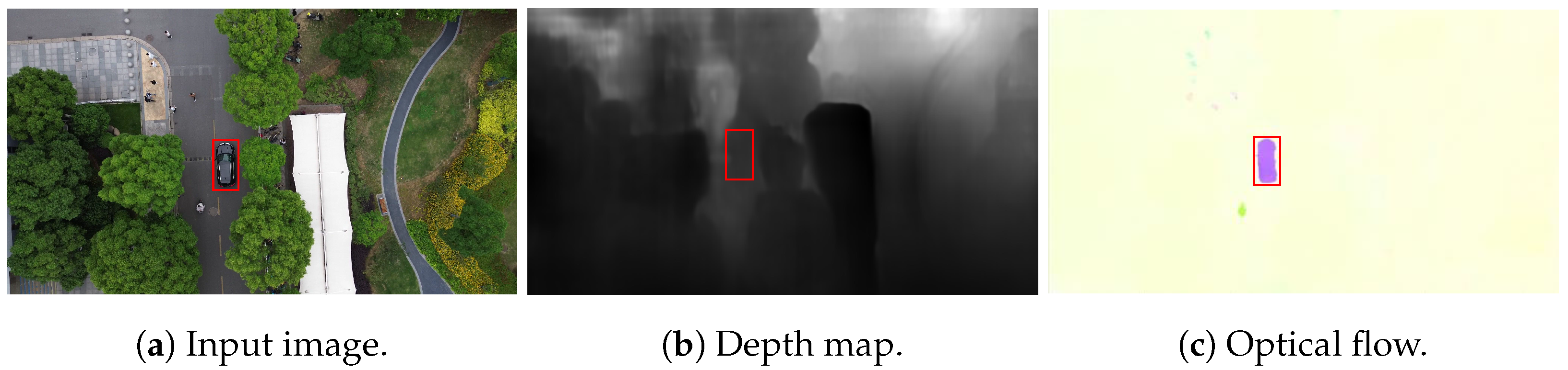
Dynamic object detection. Object detection plays a crucial role in identifying dynamic objects within a scene. For instance, buildings and trees are typically static, whereas vehicles may be either stationary or moving. By utilizing object detection results, we can further partition the semantic foreground into distinct areas, thereby facilitating the tracking of individual objects. The dynamic objects in UAV-borne images usually have fewer pixels and are mainly observed from a top-down view.

Compared to pixel-level segmentation, some first-stage object detection networks, such as the YOLO series [47], can offer notable advantages in terms of detection accuracy and speed [48]. Hence, we employ the YOLOv5 network to detect potential dynamic objects and generate object bounding boxes. Our network model used the trained weights from COCO dataset [49] and then fine-tuned them using the VisDrone dataset [50]. A trained deep network model can effectively process UAV-borne images and extract potential dynamic objects.

(2)

Monocular depth estimation. Depth estimation facilitates the retrieval of depth information for every pixel in a monocular image, which is crucial for maximizing tracked points on dynamic objects. However, dynamic objects typically occupy only a small portion of UAV-borne images. By employing estimated depth, we can densely sample the monocular images, thereby ensuring stable tracking of moving objects.

We have employed two methods to acquire scene depth. For static regions, we construct sparse maps and calculate the depth map through a triangulation algorithm. For the potential dynamic regions, we derive the depth map from monocular depth estimation. Specifically, we employ a cutting-edge monocular depth estimation method, i.e., NeW CRFs [45], to calculate the depth map. This method utilizes a novel bottom-up-top-down network architecture and has a significant improvement in the monocular depth estimation. The model is trained on the KITTI Eigen split [51]. The visualization results are shown in Figure 2b.

(3)

Optical flow estimation. Dense optical flow provides an alternative approach to establishing feature correspondences by matching sampling points across image sequences, thereby facilitating scene flow estimation. It assists in the consistent tracking of multiple objects, as the optical flow can assign an object recognition marker to each point in the dynamic region and propagate it between frames. This capability becomes particularly valuable in cases where object tracking fails, as dense flow can recover the object area.

We use PWC-Net [52] as the optical flow estimation method. The model is initially trained on the FlyingChairs dataset [53] and subsequently fine-tuned on the Sintel [54] and KITTI training datasets [55]. The visualization results are shown in Figure 2c. The deep network trained in our work can effectively extract the optical flow of targets from drone images. These optical flows form some independent rough contours of objects.

To summarize, in the preprocessing stage, we employed advanced deep network models to achieve some essential tasks, such as depth map estimation, object detection, and optical flow tracking. These network models contribute to extracting valuable information from the input images and enabling subsequent analysis.

3.3. Map Scale Restoration

Inheriting the framework of ORB-SLAM2 [6], our SLAM module uses ORB features to reconstruct a sparse environment map. Notably, UAV-borne downward-looking images contain many ground regions, facilitating the fitting of the ground plane from the 3D map points. Assuming the ground is a relatively flat region, the depth values of the ground plane fall within a certain range. To fit the ground plane, our method sorts the sparse map points in ascending order of depth value and selects theowest 40% of points. In practice, we apply the RANSAC-based fitting algorithm to calculate the plane function from the selected points. Then, we use the 2D-pixel positions corresponding to the selected 3D map points to query their depth in the depth map.

The previous calculation can only acquire a reconstructed model scale from monocular images, rather than real physical scale. Therefore, it needs to rely on additional information to restore the true scale. The height h of the camera to the ground plane can be measured using the airborne barometer. It is defined that the camera coordinate system of the first frame is consistent with the world coordinate system. The method computes the ratio between the model distance of the ground plane and the camera’s height to restore the scale of the model, as shown in Figure 3.

3.4. Object Tracking and Positioning

In the following, we derive the mathematical calculation process of object tracking. Let ${\mathbf{T}}_{{\mathrm{C}}_k\mathrm{W}}^k$, ${\mathbf{T}}_{{\mathrm{O}}_k\mathrm{W}}^k\in \mathbf{SE}\left(3\right)$ represent the camera pose and object pose in the world coordinate $\mathrm{W}$ at time k, with $k\in \mathcal{T}$ the set of time steps. To distinguish from other symbols, we use calligraphic capitaletters to represent sets of indices. Let ${\mathbf{T}}_{{\mathrm{C}}_k{\mathrm{C}}_{k-1}}^k\in \mathbf{SE}\left(3\right)$ be the homogeneous transformation of the camera motion between times $k-1$ and k. In Figure 4, the poses of cameras and objects in the world coordinate are depicted as solid curves, and their relative motion transformations are depicted as dashed curves.

Let ${\mathbf{m}}_{\mathrm{W}}^{k,i}$ be the homogeneous coordinates of the $i^{th}$ 3D point at time k, with ${\mathbf{m}}_{\mathrm{W}}^i={\left[m_x^i,m_y^i,m_z^i,1\right]}^{\mathrm{T}}\in {\mathbb{R}}^4$. The coordinate of a point in camera frame is written as ${\mathbf{m}}_{{\mathrm{C}}_k}^{k,i}={\mathbf{T}}_{{\mathrm{C}}_k\mathrm{W}}^k{·\mathbf{m}}_{\mathrm{W}}^{k,i}$. Define ${\mathrm{I}}_k$ as the image captured by the camera at time k, and let ${\mathbf{P}}_{{\mathrm{I}}_k}^i=\left[u^i,v^i,1\right]\in {\mathbb{R}}^3$ be the pixelocation on frame ${\mathrm{I}}_k$ corresponding to the homogeneous 3D point ${\mathbf{m}}_{{\mathrm{C}}_k}^{k,i}$. The imaging equation is:

$${\mathbf{P}}_{{\mathrm{I}}_k}^i=\lambda \mathbf{K}·\left({\mathbf{T}}_{{\mathrm{C}}_k\mathrm{W}}^k{·\mathbf{m}}_{\mathrm{W}}^{k,i}\right)=\lambda \mathbf{K}·{\mathbf{m}}_{{\mathrm{C}}_k}^{k,i}$$

(1)

where $\mathbf{K}$ represents the camera intrinsics. $\lambda$ indicates that a real physical scale is missing.

Firstly, we need to achieve a spatiotemporal correlation of the same objects, namely object association. The image is divided into possible dynamic regions and static regions, using the semantic information obtained from the previous object detection step. In the static regions, a set of ORB features is extracted and tracked through the feature matching method for camera pose estimation and 3D mapping. Dynamic objects usually occupy a small proportion of UAV images, which makes it difficult to track them for aong time through ORB feature points. We sample every two points within an object region and track them.

The association of dynamic objects across consecutive frames is performed by employing a combined approach. First, we use the intersection over union (IoU) of the detected object boxes [56] to perform the object-wise matching. At the same time, point-wise matching within bounding boxes is conducted by the optical flow between consecutive frames. The combination of object matching and point matching for dynamic object association can be adapted to objects of different sizes and is more robust to occlusion.

For object-wise matching, the Kalman filter is initially employed to predict theocation of tracklets in the new frame. The IoU between the detection boxes and the predicted boxes is then computed as a measure of similarity to associate high-scoring detection boxes with the tracklets. To minimize missed detections and enhance trajectory consistency, we associateow-score detection boxes with unmatched tracklets.

For the point-wise matching, let ${}_{}{}^{{\mathrm{I}}_k}\mathit{\varphi }_{}^i\in {\mathbb{R}}^2$ be the optical flow produced by the movement of the camera and objects. It represents the displacement vector of pixel ${\mathbf{P}}_{{\mathrm{I}}_{k-1}}^i$ from frame ${\mathrm{I}}_{k-1}$ to ${\mathrm{I}}_k$, and as follows:

$${}_{}{}^{{\mathrm{I}}_k}\mathit{\varphi }_{}^i={\stackrel{\sim }{\mathbf{P}}}_{{\mathrm{I}}_k}^i-{\mathbf{P}}_{{\mathrm{I}}_{k-1}}^i$$

(2)

where ${\stackrel{\sim }{\mathbf{P}}}_{{\mathrm{I}}_k}^i$ is the correspondence of ${\mathbf{P}}_{{\mathrm{I}}_{k-1}}^i$ in ${\mathrm{I}}_k$. We estimate scene flow based on optical flow, which can be used for dynamic object identification. Firstly, the scene flow ${\mathbf{f}}_k^i$ of a 3D point ${\mathbf{m}}_{\mathrm{W}}^i$ can be calculated through the camera pose ${\mathbf{T}}_{{\mathrm{C}}_k\mathrm{W}}^k$ as in [57]:

$${\mathbf{f}}_k^i={\mathbf{m}}_{\mathrm{W}}^{k-1,i}-{\mathbf{m}}_{\mathrm{W}}^{k,i}={\mathbf{m}}_{\mathrm{W}}^{k-1,i}-{{{\mathbf{T}}_{{\mathrm{C}}_k\mathrm{W}}^k}^{-1}·\mathbf{m}}_{{\mathrm{C}}_k}^{k,i}$$

(3)

Unlike optical flow, scene flow can directly decide whether some structure is moving or not. In theory, the magnitude of the scene flow vector should be zero for all static 3D points. By calculating the scene flow of sampling points in an object to determine whether it is dynamic, if the value of the scene flow of a point is greater than the set threshold, the point is considered dynamic. If the proportion of dynamic points to all points in the object area is greater than the set threshold, the object is judged as a dynamic object.

Then, we predict the motion model of an object. Let ${\mathbf{T}}_{{\mathrm{O}}_k{\mathrm{O}}_{k-1}}^k\in \mathrm{SE}\left(3\right)$ describe the homogeneous transformation of the object between times $k-1$ and k, according to:

$${\mathbf{T}}_{{\mathrm{O}}_k{\mathrm{O}}_{k-1}}^k={\mathbf{T}}_{{\mathrm{O}}_k\mathrm{W}}^k·{{\mathbf{T}}_{{\mathrm{O}}_{k-1}\mathrm{W}}^{k-1}}^{-1}$$

(4)

In Figure 4, the above motion transformations are depicted as dashed curves. A point in its corresponding object coordinates is written as ${\mathbf{m}}_{{\mathrm{O}}_k}^{k,i}={\mathbf{T}}_{{\mathrm{O}}_k\mathrm{W}}^k{·\mathbf{m}}_{\mathrm{W}}^{k,i}$, substituting the object pose at time k from Equation (4), this becomes:

$${\mathbf{m}}_{\mathrm{W}}^{k,i}={{\mathbf{T}}_{{\mathrm{O}}_k\mathrm{W}}^k}^{-1}·{\mathbf{m}}_{{\mathrm{O}}_k}^{k,i}={{\mathbf{T}}_{{\mathrm{O}}_{k-1}\mathrm{W}}^{k-1}}^{-1}·{{{\mathbf{T}}_{{\mathrm{O}}_k{\mathrm{O}}_{k-1}}^k}^{-1}·\mathbf{m}}_{{\mathrm{O}}_k}^{k,i}$$

(5)

Note that the relative positions of the points inside the rigid body remain unchanged:

$${\mathbf{m}}_{{\mathrm{O}}_k}^{k,i}={\mathbf{m}}_{{\mathrm{O}}_{k-1}}^{k-1,i}={\mathbf{T}}_{{\mathrm{O}}_{k-1}\mathrm{W}}^{k-1}{·\mathbf{m}}_{\mathrm{W}}^{k-1,i}$$

(6)

Substituting Equation (6) into Equation (5):

$${\mathbf{m}}_{\mathrm{W}}^{k,i}={{\mathbf{T}}_{{\mathrm{O}}_{k-1}\mathrm{W}}^{k-1}}^{-1}·{{\mathbf{T}}_{{\mathrm{O}}_k{\mathrm{O}}_{k-1}}^k}^{-1}·{\mathbf{T}}_{{\mathrm{O}}_{k-1}\mathrm{W}}^{k-1}·{\mathbf{m}}_{\mathrm{W}}^{k-1,i}$$

(7)

Let ${}_{k-1}{}^k\mathbf{T}_{\mathrm{W}}^{}={{\mathbf{T}}_{{\mathrm{O}}_{k-1}\mathrm{W}}^{k-1}}^{-1}·{{\mathbf{T}}_{{\mathrm{O}}_k{\mathrm{O}}_{k-1}}^k}^{-1}·{\mathbf{T}}_{{\mathrm{O}}_{k-1}\mathrm{W}}^{k-1}$, which represents the motion of the 3D point on a rigid object. The point motion in the global reference frame is then expressed as:

$${\mathbf{m}}_{\mathrm{W}}^{k,i}={}_{k-1}{}^k\mathbf{T}_{\mathrm{W}}^{}·{\mathbf{m}}_{\mathrm{W}}^{k-1,i}$$

(8)

Based on the re-projection error, we solve the object motion ${}_{k-1}{}^k\mathbf{T}_{\mathrm{W}}^{}$ by constructing a cost function. According to Equation (8), the error term is represented as:

$${\mathbf{e}}_{repr}^{k,i}={\stackrel{\sim }{\mathbf{P}}}_{{\mathrm{I}}_k}^i-\mathbf{K}·{\mathbf{T}}_{{\mathrm{C}}_k\mathrm{W}}^k·{}_{k-1}{}^k\mathbf{T}_{\mathrm{W}}^{}·{\mathbf{m}}_{\mathrm{W}}^{k-1,i}={\stackrel{\sim }{\mathbf{P}}}_{{\mathrm{I}}_k}^i-\mathbf{K}·{\mathbf{G}}^{k,i}·{\mathbf{m}}_{\mathrm{W}}^{k-1,i}$$

(9)

where ${\mathbf{G}}^{k,i}={\mathbf{T}}_{{\mathrm{C}}_k\mathrm{W}}^k·{}_{k-1}{}^k\mathbf{T}_{\mathrm{W}}^{}\in \mathrm{SE}\left(3\right)$. We parameterize the ${\mathbf{G}}^{k,i}$ by elements of theie-algebra ${\mathbf{g}}^{k,i}\in \mathrm{se}\left(3\right)$:

$${\mathbf{G}}^{k,i}=exp\left({\mathbf{g}}^{k,i}\right)$$

(10)

The optimal solution is found via minimizing:

$$\begin{array}{c}\hfill {{\mathbf{g}}^{k,i}}^{*\mathrm{V}}=\underset{{{\mathbf{g}}^{k,i}}^{\mathrm{V}}}{\mathrm{argmin}}\sum _i^{n_d}{\rho }_h\left({\mathbf{e}}_i^{\mathrm{T}}\left({\mathbf{g}}^{k,i}\right){{\sum }_p}^{-1}{\mathbf{e}}_i\left({\mathbf{g}}^{k,i}\right)\right)\end{array}$$

(11)

where $n_d$ represents the number of 3D–2D dynamic point correspondences. Here, ${\rho }_h$ is the Huber function [58], and ${\sum }_p$ is the covariance matrix related to the re-projection error. The object motion, ${}_{k-1}{}^k\mathbf{T}_{\mathrm{W}}^{}={{\mathbf{T}}_{{\mathrm{C}}_k\mathrm{W}}^k}^{-1}·{\mathbf{G}}^{k,i}$, can be recovered afterwards. This formulation enables us to jointly optimize the poses of the cameras and the dynamic objects, as well as the 3D map points.

4. Experimental Results

4.1. Experiment Setup

We collected a new dataset of visual monocular data using a UAV, as there are currently no publicly available UAV datasets specifically designed for outdoor scenarios that include dynamic objects. Our dataset aims to fill this gap in the research community by providing a valuable resource for studying and developing methods that address the challenges of dynamic object detection, tracking, and mapping in UAV-based visual systems. The data collection was conducted using the built-in monocular camera of the DJI Mini3 UAV, while the GNSS system provided navigation information. The 6D pose ground truth of the data was obtained through the aero triangulation method based on the photogrammetric software [59]. During data collection, the drone’s camera was oriented toward the ground, and the flight altitude ranged between 30 and 50 m. The collected data encompassed dynamic vehicles, pedestrians, as well as static elements such as roads, buildings, and trees. The dataset is available at https://github.com/lemonhi/UAV_dataset/tree/main (accessed on 1 March 2024).

Our method is evaluated in terms of UAVocalization and object tracking performance. The evaluation is performed on our UAV dataset and KITTI tracking dataset [60]. We use UAV data for qualitative analysis of the method and the KITTI dataset for quantitative analysis of the method. It is worth noting that even if some tests are conducted on terrain images of the KITTI dataset, they can give an insight into the general performance of our method. Due to the non-deterministic nature of running the proposed method, such as RANSAC processing, we run the SLAM algorithm five times on each sequence and take median values as the demonstrating results.

As a suggestion from reference [36], we use the translational error $E_t$ (meter) and the rotational error $E_r$ (degree) as evaluation metrics for camera pose and object motion.

4.2. Test on Our UAV Dataset

Figure 5 illustrates the output of the proposed method on our UAV dataset, showcasing a spatiotemporal map that encompasses tracks for each detected dynamic object and camera as well as static map points. The first row presents the satellite maps of the test area (the yellow curves are the UAV’s trajectories), while the bottom images show the reconstructed 3D map points (black), the trajectories of the cameras (green), and the traces of the detected objects (blue).

Throughout the UAV flights, our method demonstrates effective tracking capabilities for both the UAV-carried camera and dynamic objects in the surrounding environment. The break of the object trajectories in the DJI01 sequence is due to a missed detection caused by tree shading. When the object is detected again, the method can recover the track and map it correctly.

Figure 6 displays the estimated camera trajectories of two sequences generated by our method, alongside their corresponding ground truth trajectories. Figure 7 displays the error plots for x, y, z separately for both trajectories. The algorithm can provide a suitable estimate for the pose of the UAV. By integrating depth map estimation and optical flow estimation into our tracking framework, it becomes more resilient to occlusion andoss, providing enhanced tracking performance in challenging scenarios. Due to the use of drone barometers as reference heights, there may be a certain gap between the measured height and the actual height, which can cause errors in scale estimation.

4.3. Evaluation on the KITTI Dataset

The KITTI tracking dataset is designed for autonomous driving scenarios, but it can provide a quantitative analysis basis for the validation of drone tracking algorithms. The KITTI tracking dataset contains 21 sequences in total with ground truth for camera poses and object traces. Among these sequences, some are not included in the evaluation of our method, as they contain no obvious dynamic objects. Finally, we chose sequence Seq.00, Seq.01, Seq.02, Seq.03, Seq.04, Seq.05, Seq.06, Seq.18, and Seq.20 as our evaluation data.

(1) Evaluation of the camera poses and object motion.

Table 1. Comparison of camera pose and object trace estimation with VDO-SLAM [36] and CubeSLAM [61] on 9 sequences from the KITTI dataset. The bold numbers indicate the best result.

	CubeSLAM [61]				VDO-SLAM [36]				Ours
	Camera Pose		Object Trace		Camera Pose		Object Trace		Camera Pose		Object Trace
Seq	${\mathit{E}}_{\mathit{r}}$(deg)	${\mathit{E}}_{\mathit{t}}$(m)	${\mathit{E}}_{\mathit{r}}$(deg)	${\mathit{E}}_{\mathit{t}}$(m)	${\mathit{E}}_{\mathit{r}}$(deg)	${\mathit{E}}_{\mathit{t}}$(m)	${\mathit{E}}_{\mathit{r}}$(deg)	${\mathit{E}}_{\mathit{t}}$(m)	${\mathit{E}}_{\mathit{r}}$(deg)	${\mathit{E}}_{\mathit{t}}$(m)	${\mathit{E}}_{\mathit{r}}$(deg)	${\mathit{E}}_{\mathit{t}}$(m)
00	-	-	-	-	0.1830	0.1847	2.0021	0.3827	0.08240	0.08851	1.7187	0.5425
01	-	-	-	-	0.1772	0.4982	1.1833	0.3589	0.07378	0.1941	1.4167	0.8396
02	-	-	-	-	0.0496	0.0963	1.6833	0.4121	0.03120	0.06210	1.4527	0.6069
03	0.0498	0.0929	3.6085	4.5947	0.1065	0.1505	0.4570	0.2032	0.08360	0.1559	1.4565	0.5896
04	0.0708	0.1159	5.5803	32.5379	0.1741	0.4951	3.1156	0.5310	0.06888	0.1755	2.2280	0.8898
05	0.0342	0.0696	3.2610	6.4851	0.0506	0.1368	0.6464	0.2669	0.1371	0.0367	1.0198	1.0022
06	-	-	-	-	0.0671	0.0451	2.0977	0.2394	0.04546	0.02454	2.4642	0.9311
18	0.0433	0.0510	3.1876	3.7948	0.1236	0.3551	0.5559	0.2774	0.03618	0.09566	2.1584	0.9624
20	0.1348	0.1888	3.4206	5.6986	0.3029	1.3821	1.1081	0.3693	0.08530	0.5838	1.1869	1.2102

shows our results of both camera pose and object trace estimation compared to VDO-SLAM [36] and CubeSLAM [61] on nine image sequences. We directly used the experimental results in the paper for comparison, as we all tested using the same KITTI datasets. The CubeSLAM uses monocular images as the input to the method, while the data tested in the VDO-SLAM system include both monocular and stereo images. As our system is for monocular images, we chose the results of aearning-based monocular version of VDO-SLAM for comparison.

The translation error $E_t$ (meter) is computed as the $L_2$ norm of the translation component of relative pose error. The rotational error $E_r$ (degree) is calculated as the angle of rotation in an axis-angle representation of the rotational component of relative pose error. In comparison with VDO-SLAM, our proposed method demonstrates competitive and high accuracy in estimating camera poses. However, when it comes to object pose estimation, our method exhibits slightly higher errors than VDO-SLAM. We attribute this weaker performance in object pose estimation to the inaccuracy resulting from object detection outcomes. The detection box encompasses a small portion of the static environment, and despite our utilization of the optical flow method for filtering, certain static points are still misclassified as dynamic object points. VDO-SLAM may face challenges when dealing with extensive object occlusion, while our system has a better performance by taking advantage of the optical follow estimation.

Our method has an errorevel similar to CUbeSLAM in camera pose estimation, which may be because we are both based on the ORB-SLAM2 framework. Additionally, our method achieves slightlyower errors in object motion estimation compared to CubeSLAM, perhaps due to theoss of information caused by CubeSLAM in the process of extracting geometric models, thereby introducing uncertainty.

Figure 8 illustrates the output of our method for three of the KITTI sequences. Meanwhile, Figure 9 presents both the output map and the corresponding input image of the method running up to a specific frame within the sequence highlighted in Figure 8. This visual representation provides a clearer depiction of the system’s ability to detect and map dynamic objects. From the figures, it can be seen that our method performs relatively robustly inong-distance tracking of dynamic objects.

(2) Evaluation of the object tracking results. The performance of tracking dynamic objects is also demonstrated in our study. Figure 10 displays the results of object trackingength, which shows the selection of objects withonger trajectories. In the majority of sequences, our method achieves object trackingengths of 80% or higher. Notably, objects with trajectoryengths surpassing 200 frames, such as object 32 in Seq.05 and objects 3 and 4 in Seq.18, are successfully tracked by the system for over 80% of their duration. In this paper, optical flow estimation enables the detection and tracking of object motion by tracking pixel-level movement patterns between consecutive frames. This technique can help maintain the continuity of object tracking even in the presence of occlusions or temporaryoss of objects. The limited tracking performance observed in a small number of objects can be attributed to extensive occlusion or a significant distance from the camera.

4.4. Timing Analysis

All the experiments were conducted on a desktop computer with an Intel Core i5 2.6 GHz CPU and 16 GB RAM. In this paper, the depth estimation and optical flow results are produced offline as input to the system. The timing of our method is highly dependent on the area size and number of detected objects in the scene. In KITTI sequencesike Seq.06, there are only two objects at a time as maximum. and it can thus run at 8 fps. However, Seq.18 can have up to 15 objects at a time, and its performance is seen as slightly compromised, running at 4 fps.

Due to the scale characteristics of UAV images, dynamic objects occupy fewer pixels in the UAV dataset compared to the KITTI dataset. Thus, the proposed method is able to run at the frame rate of 7–10 fps in our UAV datasets, which have resolutions of 1920 × 1080 or 2720 × 1530. The keyframe interval in our pipeline is around 15 frames. We do not include within these numbers the time of the monocular depth estimation and dense optical flow computation since it depends on the GPU power and the model complexity.

Like most frameworks that combine SLAM and dynamic object tracking, our system may encounter scalability issues when the number of dynamic objects in the scene increases significantly. Tracking aarge number of objects simultaneously can be computationally demanding and may impact the real-time performance of the system. As the complexity of the scene increases, the computational requirements mayimit the scalability of our system.

5. Conclusions

In this paper, we present a novel dynamic monocular SLAM method for UAV flight. The proposed approach exploits image-based semantic information to seamlessly integrate object tracking within the SLAM framework, eliminating the need for prior knowledge of object pose or geometry. Depth map estimation and optical flow estimation are designed to enhance target tracking capability, particularly in scenarios involving object occlusion andoss. To evaluate the proposed algorithm, extensive experiments are performed with various UAV-borne image sequences as well as the widely used KITTI dataset. Experimental results show that our method consistently delivers robust and accurate outcomes, particularly excelling in object motion estimation. The estimated motion information of the object can be further used for subsequent tasks, such as path planning and obstacle avoidance. Therefore, our framework has been proven to be suitable for unmanned aerial vehicle visual navigation applications.

References

1. Balamurugan, G.; Valarmathi, J.; Naidu, V. Survey on UAV navigation in GPS denied environments. In Proceedings of the 2016 International Conference on Signal Processing, Communication, Power and Embedded System (SCOPES), Paralakhemundi, India, 3–5 October 2016; pp. 198–204. [Google Scholar]
2. Engel, J.; Schöps, T.; Cremers, D. SD-SLAM:arge-scale direct monocular SLAM. In Proceedings of the 13th European Conference, Zurich, Switzerland, 6–12 September 2014; pp. 834–849. [Google Scholar]
3. Forster, C.; Pizzoli, M.; Scaramuzza, D. SVO: Fast semi-direct monocular visual odometry. In Proceedings of the 2014 IEEE International Conference on Robotics and Automation (ICRA), Hong Kong, China, 31 May–7 June 2014; pp. 15–22. [Google Scholar]
4. Mur-Artal, R.; Montiel, J.M.M.; Tardos, J.D. ORB-SLAM: A versatile and accurate monocular SLAM system. IEEE Trans. Robot. 2015, 31, 1147–1163. [Google Scholar] [CrossRef]
5. Forster, C.; Zhang, Z.; Gassner, M.; Werlberger, M.; Scaramuzza, D. SVO: Semidirect visual odometry for monocular and multicamera systems. IEEE Trans. Robot. 2016, 33, 249–265. [Google Scholar] [CrossRef]
6. Mur-Artal, R.; Tardós, J.D. ORB-SLAM2: An open-source SLAM system for monocular, stereo, and RGB-D cameras. IEEE Trans. Robot. 2017, 33, 1255–1262. [Google Scholar] [CrossRef]
7. Saputra, M.R.U.; Markham, A.; Trigoni, N. Visual SLAM and structure from motion in dynamic environments: A survey. ACM Comput. Surv. (CSUR) 2018, 51, 37. [Google Scholar] [CrossRef]
8. Li, S.; Lee, D. RGB-D SLAM in dynamic environments using static point weighting. IEEE Robot. Autom. Lett. 2017, 2, 2263–2270. [Google Scholar] [CrossRef]
9. Sun, Y.; Liu, M.; Meng, M.Q.H. Improving RGB-D SLAM in dynamic environments: A motion removal approach. Robot. Auton. Syst. 2017, 89, 110–122. [Google Scholar] [CrossRef]
10. Bescos, B.; Fácil, J.M.; Civera, J.; Neira, J. DynaSLAM: Tracking, mapping, and inpainting in dynamic scenes. IEEE Robot. Autom. Lett. 2018, 3, 4076–4083. [Google Scholar] [CrossRef]
11. Xiao, L.; Wang, J.; Qiu, X.; Rong, Z.; Zou, X. Dynamic-SLAM: Semantic monocular visualocalization and mapping based on deepearning in dynamic environment. Robot. Auton. Syst. 2019, 117, 1–16. [Google Scholar] [CrossRef]
12. Bescos, B.; Neira, J.; Siegwart, R.; Cadena, C. Empty cities: Image inpainting for a dynamic-object-invariant space. In Proceedings of the 2019 International Conference on Robotics and Automation (ICRA), Montreal, QC, Canada, 20–24 May 2019; pp. 5460–5466. [Google Scholar]
13. Bešić, B.; Valada, A. Dynamic object removal and spatio-temporal RGB-D inpainting via geometry-aware adversarialearning. IEEE Trans. Intell. Veh. 2022, 7, 170–185. [Google Scholar] [CrossRef]
14. Beghdadi, A.; Mallem, M. A comprehensive overview of dynamic visual SLAM and deepearning: Concepts, methods and challenges. Mach. Vis. Appl. 2022, 33, 54. [Google Scholar] [CrossRef]
15. Fischler, M.A.; Bolles, R.C. Random sample consensus: A paradigm for model fitting with applications to image analysis and automated cartography. Commun. ACM 1981, 24, 381–395. [Google Scholar] [CrossRef]
16. Davison, A.J.; Reid, I.D.; Molton, N.D.; Stasse, O. MonoSLAM: Real-time single camera SLAM. IEEE Trans. Pattern Anal. Mach. Intell. 2007, 29, 1052–1067. [Google Scholar] [CrossRef]
17. Klein, G.; Murray, D. Parallel tracking and mapping for small AR workspaces. In Proceedings of the 2007 6th IEEE and ACM International Symposium on Mixed and Augmented Reality, Nara, Japan, 13–16 November 2007; pp. 225–234. [Google Scholar]
18. Rublee, E.; Rabaud, V.; Konolige, K.; Bradski, G. ORB: An efficient alternative to SIFT or SURF. In Proceedings of the 2011 International Conference on Computer Vision, Barcelona, Spain, 6–13 November 2011; pp. 2564–2571. [Google Scholar]
19. Zhong, F.; Wang, S.; Zhang, Z.; Wang, Y. Detect-SLAM: Making object detection and SLAM mutually beneficial. In Proceedings of the 2018 IEEE Winter Conference on Applications of Computer Vision (WACV), Lake Tahoe, NV, USA, 12–15 March 2018; pp. 1001–1010. [Google Scholar]
20. Bescos, B.; Campos, C.; Tardós, J.D.; Neira, J. DynaSLAM II: Tightly-coupled multi-object tracking and SLAM. IEEE Robot. Autom. Lett. 2021, 6, 5191–5198. [Google Scholar] [CrossRef]
21. Li, A.; Wang, J.; Xu, M.; Chen, Z. DP-SLAM: A visual SLAM with moving probability towards dynamic environments. Inf. Sci. 2021, 556, 128–142. [Google Scholar] [CrossRef]
22. Morelli, L.; Ioli, F.; Beber, R.; Menna, F.; Remondino, F.; Vitti, A. COLMAP-SLAM: A framework for visual odometry. Int. Arch. Photogramm. Remote Sens. Spat. Inf. Sci. 2023, 48, 317–324. [Google Scholar]
23. Azimi, A.; Ahmadabadian, A.H.; Remondino, F. PKS: A photogrammetric key-frame selection method for visual-inertial systems built on ORB-SLAM3. ISPRS J. Photogramm. Remote Sens. 2022, 191, 18–32. [Google Scholar] [CrossRef]
24. Jian, R.; Su, W.; Li, R.; Zhang, S.; Wei, J.; Li, B.; Huang, R. A semantic segmentation basedidar SLAM system towards dynamic environments. In Proceedings of the Intelligent Robotics and Applications: 12th International Conference (ICIRA 2019), Shenyang, China, 8–11 August 2019; pp. 582–590. [Google Scholar]
25. Zhou, B.; He, Y.; Qian, K.; Ma, X.; Li, X. S4-SLAM: A real-time 3DIDAR SLAM system for ground/watersurface multi-scene outdoor applications. Auton. Robot. 2021, 45, 77–98. [Google Scholar] [CrossRef]
26. Liu, W.; Anguelov, D.; Erhan, D.; Szegedy, C.; Reed, S.; Fu, C.Y.; Berg, A.C. SSD: Single shot multibox detector. In Proceedings of the 14th European Conference, Amsterdam, The Netherlands, 11–14 October 2016; pp. 21–37. [Google Scholar]
27. He, K.; Gkioxari, G.; Dollár, P.; Girshick, R. Mask R-CNN. In Proceedings of the 2017 IEEE International Conference on Computer Vision (ICCV), Venice, Italy, 22–29 October 2017; pp. 2961–2969. [Google Scholar]
28. Wang, C.C.; Thorpe, C.; Thrun, S. Online simultaneousocalization and mapping with detection and tracking of moving objects: Theory and results from a ground vehicle in crowded urban areas. In Proceedings of the 2003 IEEE International Conference on Robotics and Automation (Cat. No.03CH37422), Taipei, Taiwan, 14–19 September 2003; pp. 842–849. [Google Scholar]
29. Wangsiripitak, S.; Murray, D.W. Avoiding moving outliers in visual SLAM by tracking moving objects. In Proceedings of the 2009 IEEE International Conference on Robotics and Automation, Kobe, Japan, 12–17 May 2009; pp. 375–380. [Google Scholar]
30. Kundu, A.; Krishna, K.M.; Jawahar, C. Realtime multibody visual SLAM with a smoothly moving monocular camera. In Proceedings of the 2011 International Conference on Computer Vision, Barcelona, Spain, 6–13 November 2011; pp. 2080–2087. [Google Scholar]
31. Reddy, N.D.; Singhal, P.; Chari, V.; Krishna, K.M. Dynamic body VSLAM with semantic constraints. In Proceedings of the 2015 IEEE/RSJ International Conference on Intelligent Robots and Systems (IROS), Hamburg, Germany, 28 September–2 October 2015; pp. 1897–1904. [Google Scholar]
32. Bârsan, I.A.; Liu, P.; Pollefeys, M.; Geiger, A. Robust dense mapping forarge-scale dynamic environments. In Proceedings of the 2018 IEEE International Conference on Robotics and Automation (ICRA), Brisbane, QLD, Australia, 21–25 May 2018; pp. 7510–7517. [Google Scholar]
33. Huang, M.; Wu, J.; Zhiyong, P.; Zhao, X. High-precision calibration of wide-angle fisheyeens with radial distortion projection ellipse constraint (RDPEC). Mach. Vis. Appl. 2022, 33, 44. [Google Scholar] [CrossRef]
34. Huang, J.; Yang, S.; Zhao, Z.; Lai, Y.K.; Hu, S.M. ClusterSLAM: A SLAM backend for simultaneous rigid body clustering and motion estimation. In Proceedings of the 2019 IEEE/CVF International Conference on Computer Vision (ICCV), Seoul, Republic of Korea, 27 October–2 November 2019; pp. 5875–5884. [Google Scholar]
35. Henein, M.; Zhang, J.; Mahony, R.; Ila, V. Dynamic SLAM: The need for speed. In Proceedings of the 2020 IEEE International Conference on Robotics and Automation (ICRA), Paris, France, 31 May–31 August 2020; pp. 2123–2129. [Google Scholar]
36. Zhang, J.; Henein, M.; Mahony, R.; Ila, V. VDO-SLAM: A visual dynamic object-aware SLAM system. arXiv 2020, arXiv:2005.11052. [Google Scholar] [CrossRef]
37. Shan, M.; Wang, F.; Lin, F.; Gao, Z.; Tang, Y.Z.; Chen, B.M. Google map aided visual navigation for UAVs in GPS-denied environment. In Proceedings of the 2015 IEEE International Conference on Robotics and Biomimetics (ROBIO), Zhuhai, China, 6–9 December 2015; pp. 114–119. [Google Scholar]
38. Zhuo, X.; Koch, T.; Kurz, F.; Fraundorfer, F.; Reinartz, P. Automatic UAV image geo-registration by matching UAV images to georeferenced image data. Remote Sens. 2017, 9, 376. [Google Scholar] [CrossRef]
39. Volkova, A.; Gibbens, P.W. More robust features for adaptive visual navigation of UAVs in mixed environments: A novelocalisation framework. J. Intell. Robot. Syst. 2018, 90, 171–187. [Google Scholar] [CrossRef]
40. Kim, Y. Aerial map-based navigation using semantic segmentation and pattern matching. arXiv 2021, arXiv:2107.00689. [Google Scholar] [CrossRef]
41. Couturier, A.; Akhloufi, M.A. A review on absolute visualocalization for UAV. Robot. Auton. Syst. 2021, 135, 103666. [Google Scholar] [CrossRef]
42. Qin, T.; Shen, S. Robust initialization of monocular visual-inertial estimation on aerial robots. In Proceedings of the 2017 IEEE/RSJ International Conference on Intelligent Robots and Systems (IROS), Vancouver, BC, Canada, 24–28 September 2017; pp. 4225–4232. [Google Scholar]
43. Qin, T.; Li, P.; Shen, S. VINS-mono: A robust and versatile monocular visual-inertial state estimator. IEEE Trans. Robot. 2018, 34, 1004–1020. [Google Scholar] [CrossRef]
44. Fu, Q.; Wang, J.; Yu, H.; Ali, I.; Guo, F.; He, Y.; Zhang, H. PL-VINS: Real-time monocular visual-inertial SLAM with point andine features. arXiv 2020, arXiv:2009.07462. [Google Scholar] [CrossRef]
45. Yuan, W.; Gu, X.; Dai, Z.; Zhu, S.; Tan, P. New CRFs: Neural window fully-connected CRFs for monocular depth estimation. arXiv 2022, arXiv:2203.01502. [Google Scholar] [CrossRef]
46. Kalman, R.E. A new approach toinear filtering and prediction problems. J. Basic Eng. 1960, 82D, 35–45. [Google Scholar] [CrossRef]
47. Redmon, J.; Divvala, S.; Girshick, R.; Farhadi, A. You onlyook once: Unified, real-time object detection. In Proceedings of the 2016 IEEE Conference on Computer Vision and Pattern Recognition (CVPR), Las Vegas, NV, USA, 27–30 June 2016; pp. 779–788. [Google Scholar]
48. Zaidi, S.S.A.; Ansari, M.S.; Aslam, A.; Kanwal, N.; Asghar, M.; Lee, B. A survey of modern deepearning based object detection models. Digit. Signal Process. 2022, 126, 103514. [Google Scholar] [CrossRef]
49. Lin, T.Y.; Maire, M.; Belongie, S.; Hays, J.; Perona, P.; Ramanan, D.; Dollár, P.; Zitnick, C.L. Microsoft COCO: Common objects in context. In Proceedings of the 13th European Conference, Zurich, Switzerland, 6–12 September 2014; pp. 740–755. [Google Scholar]
50. Zhu, P.; Wen, L.; Du, D.; Bian, X.; Fan, H.; Hu, Q.; Ling, H. Detection and tracking meet drones challenge. IEEE Trans. Pattern Anal. Mach. Intell. 2021, 44, 7380–7399. [Google Scholar] [CrossRef]
51. Eigen, D.; Puhrsch, C.; Fergus, R. Depth map prediction from a single image using a multi-scale deep network. arXiv 2014, arXiv:1406.2283. [Google Scholar] [CrossRef]
52. Sun, D.; Yang, X.; Liu, M.Y.; Kautz, J. PWC-net: CNNs for optical flow using pyramid, warping, and cost volume. In Proceedings of the 2018 IEEE/CVF Conference on Computer Vision and Pattern Recognition, Saltake City, UT, USA, 18–23 June 2018; pp. 8934–8943. [Google Scholar]
53. Mayer, N.; Ilg, E.; Hausser, P.; Fischer, P.; Cremers, D.; Dosovitskiy, A.; Brox, T. Aarge dataset to train convolutional networks for disparity, optical flow, and scene flow estimation. In Proceedings of the 2016 IEEE Conference on Computer Vision and Pattern Recognition (CVPR), Las Vegas, NV, USA, 27–30 June 2016; pp. 4040–4048. [Google Scholar]
54. Butler, D.J.; Wulff, J.; Stanley, G.B.; Black, M.J. A naturalistic open source movie for optical flow evaluation. In Proceedings of the 12th European Conference on Computer Vision, Florence, Italy, 7–13 October 2012; pp. 611–625. [Google Scholar]
55. Geiger, A.; Lenz, P.; Urtasun, R. Are we ready for autonomous driving? The KITTI vision benchmark suite. In Proceedings of the 2012 IEEE Conference on Computer Vision and Pattern Recognition, Providence, RI, USA, 16–21 June 2012; pp. 3354–3361. [Google Scholar]
56. Zhang, Y.; Sun, P.; Jiang, Y.; Yu, D.; Weng, F.; Yuan, Z.; Luo, P.; Liu, W.; Wang, X. ByteTrack: Multi-object tracking by associating every detection box. In Proceedings of the 17th European Conference, Tel Aviv, Israel, 23–27 October 2022; pp. 1–21. [Google Scholar]
57. Lv, Z.; Kim, K.; Troccoli, A.; Sun, D.; Rehg, J.M.; Kautz, J. earning rigidity in dynamic scenes with a moving camera for 3D motion field estimation. In Proceedings of the 15th European Conference on Computer Vision, Munich, Germany, 8–14 September 2018; pp. 468–484. [Google Scholar]
58. Huber, P.J. Robust estimation of aocation parameter. In Breakthroughs in Statistics: Methodology and Distribution; Springer: Berlin/Heidelberg, Germany, 1992; pp. 492–518. [Google Scholar]
59. Agistoft, LLC. Agisoft Metashape. 2023. Available online: https://www.agisoft.com/zh-cn/downloads/installer (accessed on 1 May 2023).
60. Geiger, A.; Lenz, P.; Stiller, C.; Urtasun, R. Vision meets robotics: The KITTI dataset. Int. J. Robot. Res. 2013, 32, 1231–1237. [Google Scholar] [CrossRef]
61. Yang, S.; Scherer, S. CubeSLAM: Monocular 3D object SLAM. IEEE Trans. Robot. 2019, 35, 925–938. [Google Scholar] [CrossRef]
Figure 1. Overview of the visual SLAM method.
Drones 08 00222 g001
Figure 2. Visualization results of the pre-processing module.
Drones 08 00222 g002
Figure 3. Restore scale information based on height ratio. The grey region in the middle represents a ground plane using a RANSAC-based fitting algorithm.
Drones 08 00222 g003
Figure 4. The dynamic object tracking process between airborne images.
Drones 08 00222 g004
Figure 5. Illustration of the results on the UAV dataset. The first row presents the satellite maps of the test area, while the bottom images show the corresponding maps (2.8 points/m2) and the trajectories of cameras and objects. (Image numbers and resolution: DJI01, 272 keyframes, 1920 × 1080; DJI02, 340 keyframes, 2720 × 1530; DJI03, 272 keyframes, 2720 × 1530; DJI04, 370 keyframes, 2720 × 1530).
Drones 08 00222 g005
Figure 6. Trajectories on the sequences DJI01 and DJI04.
Drones 08 00222 g006
Figure 7. The error plots for x, y, z separately for both trajectories.
Drones 08 00222 g007
Figure 8. Illustration of the results on the KITTI dataset. (Topeft: Seq.03, top right: Seq.18, and bottom: Seq.20).
Drones 08 00222 g008
Figure 9. Illustration of system map for a certain frame and corresponding image. The bounding box and the speed of the objects are inferred in the image. The left figure represents Seq.03, the middle figure represents Seq.18, and the right figure represents Seq.20.
Drones 08 00222 g009
Figure 10. Tracking performance. Results of object trackingength for some selected objects (tracked for over 20 frames) due toimited space. The color bars represent the number of objects appearing in the image. “GT” refers to ground truth and “EST.” refers to estimated values.“Sequence” represents the sequence number of the KITTI dataset used in the experiment, and “Object id” represents the dynamic object id that appears in the sequence.
Drones 08 00222 g010