Estimation Method of Chlorophyll Concentration Distribution Based on UAV Aerial Images Considering Turbid Water Distribution in a Reservoir

Abstract

The observation of the phytoplankton distribution with a high spatiotemporal resolution is necessary to track the nutrient sources that cause algal blooms and to understand their behavior in response to hydraulic phenomena. Photography from UAVs, which has an excellent temporal and spatial resolution, is an effective method to obtain water quality information comprehensively. In this study, we attempted to develop a method for estimating the chlorophyll concentration from aerial images using machine learning that considers brightness correction based on insolation and the spatial distribution of turbidity evaluated by satellite image analysis. The reflectance of harmful algae bloom (HAB) was different from that of phytoplankton seen under normal conditions; so, the images containing HAB were the causes of error in the estimation of the chlorophyll concentration. First, the images when the bloom occurred were extracted by the discrimination with machine learning. Then, the other images were used for the regression of the concentration. Finally, the coefficient of determination between the estimated chlorophyll concentration when no bloom occurred by the image analysis and the observed value reached 0.84. The proposed method enables the detailed depiction of the spatial distribution of the chlorophyll concentration, which contributes to the improvement in water quality management in reservoirs.

1. Introduction

In enclosed water bodies, such as lakes, bays, and reservoirs, the water exchange is gradual, so that the nutrients of nitrogen and phosphorus flowing in from the catchment area tend to accumulate [1]. When particulate phosphorus is deposited deep down, it takes on complex dynamics due to the stratification of the water body. When nutrients eluted by internal flow are delivered to a field with a suitable water temperature and illuminance conditions, the bloom of phytoplankton occurs in a field that is spatiotemporally different from the direct supply of nutrients [2,3,4]. The predominance of certain species of phytoplankton can cause taste and odor problems that contribute to the degradation of drinking water supplies, inhibit recreational uses of surface waters [5], and reduce suitable fish habitats, and some assemblages of cyanobacteria produce toxins that are harmful to humans and animals [6,7]. In eutrophic lakes, the species of the Microcystis genus, which have gas vesicles, often dominate and spread on the whole water surface. Harmful algal bloom (HAB) is considered a social problem that poses a major hindrance to the environment and human activities [8,9,10,11,12].

One of the fundamental countermeasures against this problem is to identify the toxic species and find the environmental variation patterns in which the species occur. Houliez et al. [13] identified the assemblage composition of phytoplankton and studied the temporal variability in photosynthetic activity in the coastal waters of the Strait of Dover and related it to the environmental conditions. Azevedo et al. [14] studied the spatial and temporal characterization of key environmental variables aiming at the design of a conceptual model of the Douro estuary. Perry et al. [15] surveyed domoic acid and Pseudo-nitzschia spp. from 2016 to 2021 in the Pacific waters of Canada to assess their occurrences, concentrations, and relationships with physical and chemical conditions.

Controlling environmental factors, such as the supply of nutrients, so that they do not exceed thresholds that could lead to algal bloom is the solution for this issue, while it is difficult to control the other factors of the blooming, i.e., insolation and the water temperature in water bodies. There have been many attempts to predict the abnormal occurrence of phytoplankton blooming based on machine learning from various water quality parameters. Tian et al. [16] proposed the novel HAB prediction index based on the catastrophe theory. Shan et al. [17] developed a Bayesian modeling framework with intracellular and extracellular MCs that characterizes the relationships between different environmental and biological factors. Wang et al. [18] introduced the multivariate timing-random deep belief net model that combined multifactor time series analysis and deep belief net and validated it with data collected in Lake Taihu.

However, as mentioned above, the spatiotemporal behavior of the nutrients within a water body is complex. Even if the species identification and water quality analysis are performed using water sampled at a limited number of locations in a water body, achieving this goal is difficult. Corresponding to the site and the phenomena, large-scale efforts and cost-intensive investigations are required. Wang et al. [19] analyzed the relationship between the abundance of picophytoplankton and environmental factors. They revealed that the picophytoplankton distribution was strongly correlated with the degree of the vertical stratification of the water column. Jiang et al. [20] collected water samples from the surface of Lake Chaohu and the rivers around the lake to characterize the seasonal variation and spatial distribution of the phytoplankton community structure. Dale et al. [21] presented a 33-year phytoplankton survey program at a greater density of stations than other published surveys. The results suggested limitations that should be recognized in the use of lower-resolution records when evaluating HABs, modeling HABs, and attempting long-term predictions of HABs. Nwe et al. [22] analyzed the variation in cell size distribution and phytoplankton habitats according to the hydrodynamic conditions in an estuary. The water samples were collected at six stations for analyzing phytoplankton species, while the vertical profile of salinity, temperature, turbidity, and light intensity were measured using a CTD probe, turbidity, and light sensors with a 0.1 m vertical interval. Chaffin et al. [23] determined how well water quality sondes attached to buoys measure the distribution of algae and cyanobacterial biomass. It was useful as a guidance tool for sectors like water treatment and beach management.

On the other hand, the sophistication of the simulations in hydrodynamics and its associated changes in water quality have progressed rapidly in recent years. The reproducibility and the spatiotemporal resolution of the distributions within a water body have become reliable and have a high precision [24,25,26,27]. Several studies have forecast the HAB occurrence based on water quality simulated by these hydrodynamic models [28,29,30]. Jin et al. [31] proposed the method of applying convolutional neural networks to the simulated spatial distribution of the water quality parameters to estimate the spatial distribution of chlorophyll-a. In proportion to these trends, the development of observation technology with a high spatiotemporal resolution for HABs is expected. This is because the distribution of HABs can change rapidly due to variations in population dynamics and environmental conditions. Normal water quality analysis and microscopic observation require a large amount of time and labor, even for only one sample; so, it is difficult to understand the entire dynamics of HABs. Except for the above example that carried out considerable sampling and analysis of water, there are very few cases in which a sufficient number of observations have been made to enable discussion about the transportation of nutrients by currents within a water body.

Remote sensing enables to obtain the spatiotemporally high-density observations required for HAB monitoring in a wide area of water at a relatively low cost. This is because phytoplankton generally proliferates only in shallow layers where sunlight reaches the surface of the water. In addition, the species of the Microcystis genus, which is one of the groups of HAB, float using gas vesicles. Therefore, it is highly compatible with the use of remote sensing from the sky, which measures the intensity of reflection on the water surface layers, especially in large lakes and coastal areas. Mamun et al. [32] developed empirical models from Landsat 5 TM data to monitor the total phosphorus, BOD, and chlorophyll-a. Li et al. [33] used multiple satellite image analyses to observe the green tide, which occurs in the southern Yellow Sea and moves northward, severely impacting the coastal ecological environment. Hu et al. [34] developed an objective method to estimate the biomass of Ulva prolifera using satellite image analysis and clarified the transition of its blooming area. Mugani et al. [35] calculated the normalized difference vegetation index (NDVI) using multi-sensor Landsat imagery and established a historical record of cyanobacterial activity in the reservoir spanning 30 years to identify patterns and trends in cyanobacterial proliferation.

In general, satellite data, such as MODIS, that come in every day has a coarse spatial resolution, while satellites with a high spatial resolution, such as Sentinel, come in once every 1–2 weeks. Through the passive multi-band sensors mounted on the above satellites, images can be captured only when the sky is clear on that day. In satellite image analysis, it is often necessary to choose either spatial or temporal resolution. Chen et al. [36] calculated FAI based on Advanced Himawari Imager (AHI) data acquired by the geostationary meteorological satellite for the detection of the diurnal algae dynamics in Lake Tai, China. The observations by geostationary satellites have a guaranteed exceptionally high resolution and imaging frequency. However, such satellite data are not obtained in every region. In analyses based on data from global observation satellites, which can be applied anywhere, it is necessary to select either spatial resolution or inbound frequency depending on the characteristics of the research objects. To supplement this, there are examples of combining various types of satellite images and discussing the short-term decline in HABs. Liu et al. [37] calculated the floating algae index (FAI) from Sentinel-2 MSI and Landsat-8 OLI images to monitor the spatial and seasonal variability in floating algae in a small lake from 2016 to 2020. The consistency of the FAI between MSI and OLI was confirmed, and the FAI threshold to distinguish floating algae was found using a bimodal histogram; the results suggest that the spatial distributions based on the different satellites can also be used in common.

Most of the studies on the wide-area observation of HABs using satellite images have mainly focused on natural lakes, rivers, and seawater, and only a few studies have been conducted on reservoirs, even though the water quality management of a reservoir is extremely important for the supply of drinking water [38,39,40]. The reason is due to the characteristics of each observation method mentioned above. The reservoirs in mountainous areas are smaller than the ocean, and satellites such as MODIS, which frequently take images, have an insufficient resolution. Alternatively, if a satellite has a certain high spatial resolution, the imaging interval will be weekly, making it impossible to track the dynamics of phytoplankton. In particular, images of reservoirs located in mountainous areas are often difficult to obtain due to cloud cover.

To compensate for this drawback of satellite image analyses, it is preferable to analyze aerial images taken from unmanned aerial vehicles (UAVs) and collect images with a spatiotemporally high resolution. This research aims to conduct observations using photographs taken from an UAV and to be able to conduct a spatially high-resolution analysis freely without restrictions due to photographing date or cloud cover [41,42]. Using a small UAV system equipped with a consumer-grade camera, Qu et al. [43] determined surface-floating cyanobacteria at a maximum detection altitude of 80 m. The small UAV can cover up to 1 km² per flight mission, and the short time lag between sampling and flight allows for follow-up monitoring and treatment. Guimarães et al. [44] photographed a small reservoir with an NGB (near-infrared (N), green (G), and blue (B)) camera connected to an UAV and extracted NDVI from orthorectified images. The results of the multivariate analysis using each spectrum data as an explanatory variable and NDVI showed some correlations with the chlorophyll-a (Chl-a) concentration. Su et al. [45] tried the estimation of the concentration of Chl-a and total phosphate and using the average method and pixel-by-pixel matching (MPP) method to search for the optimal regression model from the brightness values of multispectral images obtained by an UAV. In each of these research cases, the study site was narrower than in the research based on satellite image analysis, and the observations were completed with a limited number of images.

However, the fluctuations in insolation strongly affect the analysis results. In addition, because reservoirs are generally narrow and laterally long, there is a spatial distribution of turbidity depending on the distance from the river inflow and the season, which affects the color tone. This tends to cause errors in determining the Chl-a concentration. In a reservoir, a narrow and closed water body that has some river inflow, it is also necessary to be able to observe the spatial distribution of low-ranging chlorophyll in the pre-occurrence stage of HABs to determine the source of nutrients. Cheng et al. [46] developed an estimation model for the Chl-a concentration from the images taken by a digital camera mounted on an UAV and validated the estimated results against the observed data over a year. As the photography duration increases, the insolation conditions change in a day, and the insolation conditions also differ if the photography takes place on different days and in different seasons; so, the brightness value of the photograph changes even for the same color on the water surface. In the study, the brightness values of each spectrum were corrected based on the amount of insolation. The need to correct insolation conditions is an issue not only for aerial images taken by UAVs but also when comparing images taken on different dates in satellite image analysis [37,47,48].

In addition to the insolation and Chl-a, turbidity and colored dissolved organic matter (CDOM) are the factors that greatly affect the color of water surfaces. Kishino et al. [49] proposed using a neural network to estimate the concentration of turbidity and Chl-a simultaneously from images taken by the Aster satellite. Sakuno et al. [50] developed an integrated algorithm for the remote sensing of Chl-a and turbidity in eutrophic and hyper-turbid waters, such as Lake Shinji and Nakaumi in Japan and the Vaal Dam Reservoir in South Africa. Palmer et al. [51] investigated indicators for evaluating the distribution of the Chl-a concentration in shallow lakes with extremely high turbidity. Alcântara et al. [52] tested the potential of the red–blue–green ratio for predicting aCDOM (440) from Landsat-8 images. The ratio of red/blue showed the best performance to estimate CDOM in the study. On the other hand, in the study of Glukhovets et al. [53], which estimated the absorption coefficient of CDOM in the northern seas from OLCI data from Sentinel-3 satellites, it was shown that the real uncertainties are significantly high due to the unsatisfactory atmospheric correction.

This study proposes calibration methods for the factors affecting the colors on aerial images. The flight altitude of an UAV is low, and so clouds are not obstacles when shooting. However, considerable shooting is required to cover the whole lake and it takes a longer time; so, the insolation conditions change drastically during the observation. In addition, there are turbid water inflows to a reservoir. First, the calibration of the reflectance of the images due to insolation is introduced. Then, we investigate a method for estimating the Chl-a concentration using machine learning based on the calibrated reflectance values and estimated turbidity by the satellite image analysis. Not only was the presence or absence of the bloom of HABs identified, but the distribution of the lower concentrations of Chl-a, that is, the information expected as a fundamental solution, was also assessed.

2. Materials and Methods

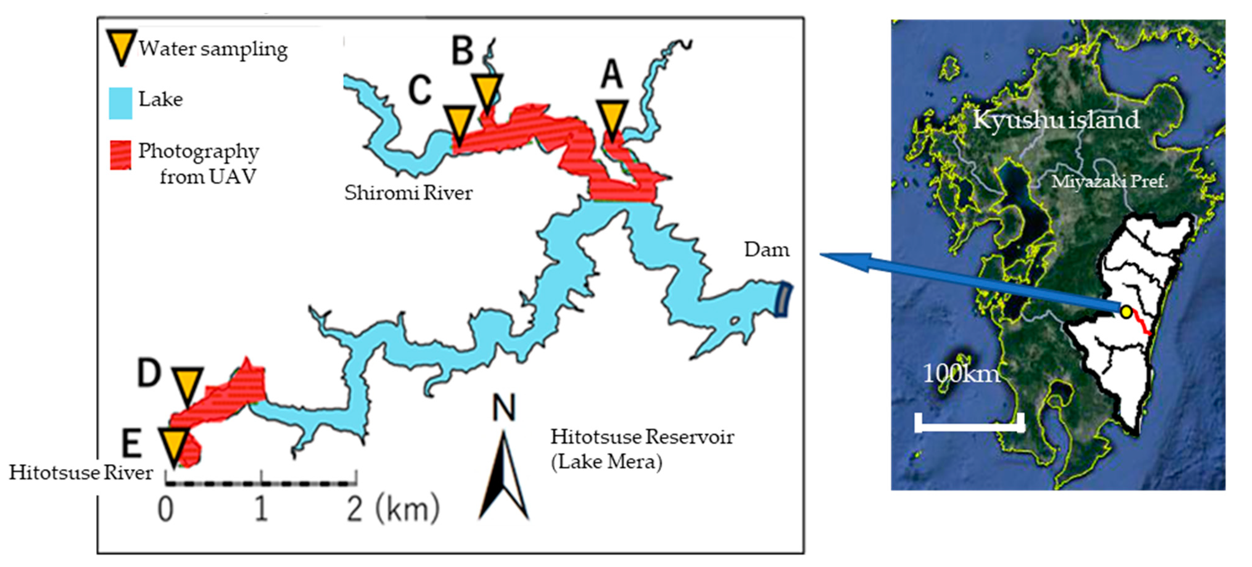
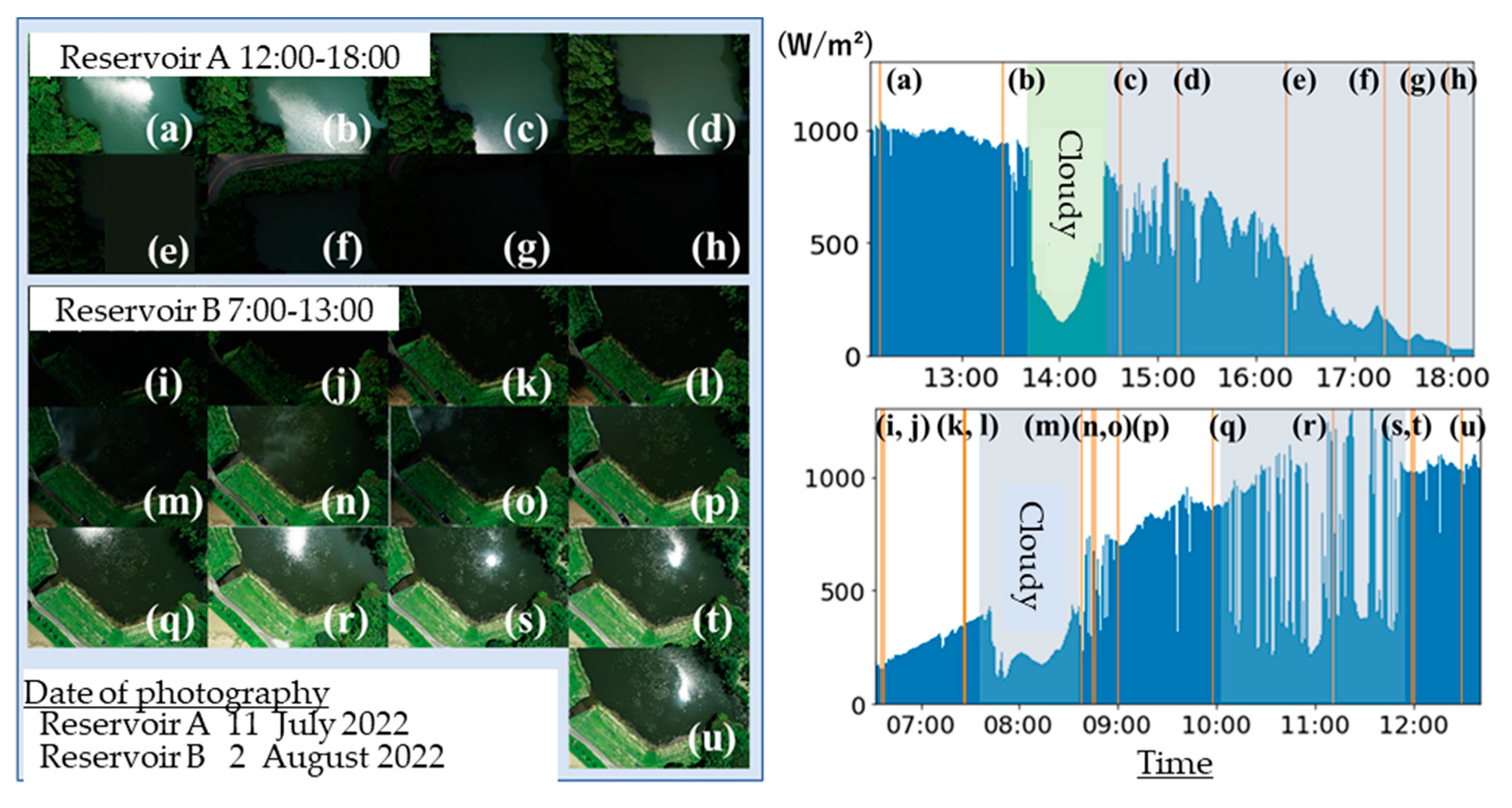
2.1. Study Site and Photography from the UAV

The study site was the Hitotsuse Reservoir (total storage capacity: 264,315,000 m³; catchment area: 445 km²), upstream of the Hitotsuse River in Miyazaki Prefecture, Japan (Figure 1). UAV aerial photography surveys were conducted 10 times from 25 September 2020 to 23 October 2022. The UAV aerial photography area is indicated by the red hatched area in Figure 1, and the locations where the water quality surveys were conducted are indicated by the yellow reverse triangles (A to E). The water sampling and the vertical profiling of water quality were conducted from the bridges spanning these points.

Microcystis bloom has been frequently confirmed in the reservoir in the past. Among the above observations, the bloom was visually confirmed during the survey on 16 July 2022, but it was not found during the other observations.

Phantom 4 pro-V2.0 manufactured by DJI was used to take aerial photographs near the inlet of the Shiromi River and Hitotsuse River, shown as the red-colored area in Figure 1. Figure 2 shows the shooting settings using the UAV-equipped digital camera. The images were taken at a flight altitude of 140 m, with overlap rates of 90% on the route and 50–60% between the routes. The number of pixels (pix) of the digital camera was 5472 × 3648 pixels. The size of the image sensor that converts red, blue, and green visible lights into electrical signals was 13.2 × 8.8 mm. The lens focal length was 9.0 mm.

During a flight lasting from 15 to 30 min, the brightness of the images fluctuated depending on the change in cloud cover and the solar angle, varying with the shooting date and time. To calibrate the reflectance in the images, the insolation was measured with a pyranometer (ML-01, Eiko Seiki Co., Ltd., Tokyo, Japan) near each water quality survey point at 5 s intervals in parallel with the flight.

2.2. Water Sampling and Vertical Profiling

Fluorescence measurements of chlorophyll and turbidity were carried out by lowering a water quality profiler (AAQ-RINKO, JFE Advantech, Kobe, Japan) from the bridges over the five points shown in Figure 1. At the same time, the water was sampled from a depth of 2 m and the concentration of Chl-a was measured by the SCOR-UNESCO method. Five liters of the water sample were filtered through a glass fiber filter (Whatman, GF/F, Diameter 47 mm). The residue was extracted with 30 mL of 99.5% ethanol, placed in a 50 mL centrifuge tube protected from light by aluminum foil, and refrigerated for 24 h. Afterward, it was centrifuged at 3000 rpm for 5 min. The supernatant liquid was put into a glass cell (5 cm), and the absorbance was measured at the wavelengths of 750, 663, 645, and 630 nm. The concentration of Chl-a was calculated as the equation below.

$$\mathrm{C}\mathrm{h}\mathrm{l}-\mathrm{a}=11.64\times \mathrm{e}663-2.16\times \mathrm{e}645+0.10\times \mathrm{e}630$$

(1)

where e663, e645, and e630 are the absorbances for each wavelength. Since the Chl-a concentration obtained by the fluorescence measurement with the profiler was the Uranine reference value, the calibration formula between the Chl-a concentration of the water sample measured by the SCOR-UNESCO method and the Uranine reference value measured at the same depth by the profiler was identified. The value measured with the profiler was converted to the Chl-a concentration with this calibration formula. Figure 3 shows the calibration formula between the Chl-a concentration by the SCOR-UNESCO method and the fluorescence intensity of the Uranine concentration reference by the profiler. There was a good correlation between the two values, except for the day when the Microcystis bloom occurred (16 July 2022).

2.3. Distribution of Turbidity

In the subsequent sections, the observed concentration of Chl-a at a depth of 1 m will be estimated by machine learning regression with the calibrated RGB reflectance values and other additional explanatory parameters. Hereafter, the turbidity is incorporated as the explanatory parameter because it is considered to be a factor, in addition to the Chl-a concentration, that influences the hue of the lake water surface. Figure 4 shows the turbidity (marks) and water temperature (bars) measured at a depth of 1 m on each observation day. There are cases in which the turbidity differs significantly between the Shiromi River (points A, B, and C) and the Hitotsuse River (points D and E) even on the same day. The spatial distribution of the turbidity occurs due to the differences in the turbidity loaded from each inflowing river and the behavior of the turbid water after the inflow.

It is necessary to measure the turbidity of the entire lake water surface directly to take into account the factor of the hue, which is putting the cart before the horse. In this study, the spatial distribution of the turbidity was estimated using the water turbidity index (WTI) [54]. The WTI was calculated using the red and near-infrared bands of the Sentinel-2 satellite (spatial resolution: 10 m) and Landsat satellite data (30 m). The dates of these satellite images do not match those of the UAV aerial photography. However, it has been reported that the Hitotsuse River basin has a geological structure that is prone to prolonged turbidity [55,56], and its spatial distribution changes are gentler than those in Chl-a. If the temporal gap between the two images is less than one week, and there is no flooding during that time, it is considered that the satellite images are almost synchronized with the UAV aerial images. The WTI was calculated using Equations (2)–(7) shown below.

First, the minimum value (Ref_min) is subtracted from the maximum value (Ref_max) of the red band (RED) and near-infrared (NIR) reflectance.

$$b_{RED}={\left({Ref}_{max}-{Ref}_{min}\right)}_{\mathrm{R}\mathrm{E}\mathrm{D}}$$

(2)

$$b_{NIR}={\left({Ref}_{max}-{Ref}_{min}\right)}_{\mathrm{N}\mathrm{I}\mathrm{R}}$$

(3)

In each band, b_RED and b_NIR are normalized. The normalized coefficients A_RED and A_NIR are obtained, divided by the normalized coefficient B. Finally, WTI is calculated by multiplying the reflectance of the red band and near-infrared image by the normalized coefficients.

$$B=\sqrt{b_{RED}^2+b_{NIR}^2}$$

(4)

$$A_{RED}=\frac{b_{RED}}{B}$$

(5)

$$A_{NiR}=\frac{b_{NIR}}{B}$$

(6)

$${WTI}_i=A_{RED}{Ref}_{RED}+A_{NIR}{Ref}_{NIR}$$

(7)

CDOM, which is another factor that affects the color of the water surface, is not considered in this case as a direct explanatory variable. This is because both the inflowing waters from the rivers and lake water are so clear that it can be visually determined as less CDOM. There are no large resources of humic substances, such as peatlands in the basin; so, the inflowing river water is clear. The retention time of the lake water is approximately 2–3 months. During such a short period of time, it is rare to elute high concentrations of humic substances. However, since the possibility of some seasonal fluctuations cannot be denied, the water temperature was added in this case as an index of seasonal fluctuations not only in CDOM but also in all other unknown factors.

2.4. The Flow Chart of the Overall Processes for Machine Learning

Gradient boosting was applied for the classification of the presence of bloom and the regression of the Chl-a concentration at a 1 m depth, with the calibrated RGB reflectance, temperature, and WTI. In addition, the weak classifier used in this case was a decision tree. Decision trees are well known for their use in classification, but they can also be used in regression. The gradient boosting that utilizes this decision tree is called gradient boosting decision tree (GBDT), and a faster version of this algorithm is called extreme gradient boosting (XGBoost) [57]. In this research, we applied XGBoost to improve the accuracy of classifying the presence or absence of Microcystis and predicting the concentration of Chl-a in the stage before blooming by the regression.

Figure 5 shows the flow of the machine learning algorithm. The RGB reflectance calibrated by insolation, WTI values obtained from satellite images, and the water temperature were used as input parameters. Since the water temperature was uniform over the entire lake surface on each survey day, the observed value at point E was used as the representative value. First, we used XGBoost and these parameters to try to determine the presence or absence of the bloom. This is because when the bloom occurred, the fluorescence characteristics of chlorophyll were different from those under normal conditions, as shown in Figure 3; so, it was thought that the reflectance of the visible lights on the water surface would show a unique state. The purpose of this research is not only to determine the presence or absence of blooms but also to investigate the causes of their occurrence through normal-time observations that show the distribution of Chl-a concentrations at lower concentrations. Therefore, we attempted to reproduce the Chl-a concentration using the XGBoost regression model for the images that were determined to be free of bloom.

In this study, the number of field surveys was limited. To obtain a sufficient number of datasets for the training and assessment of the machine learning, we extracted 25 pixels from an area of 3.3 × 3.3 m around the water quality meter point of the image at each point and used their RGB values as the parameters. The mesh size of the WTI was 10 × 10 m. On the other hand, as shown in Figure 6, it is confirmed that there is some variation in the RGB dataset. Based on this, we increased the data used for machine learning by preparing 25 types of RGB datasets for one WTI value, water temperature, and Chl-a concentration. Therefore, 1000 sets (25 × 5 points × 8 observation days) were used for classification, and 875 sets (25 × 5 locations × 7 days) were used for regression.

The values of the calibrated RGB reflectance, WTI, and water temperature were normalized by the Min-Max method, scaling the data from 0 to 1 as shown in Equation (8). Normalization was expected to improve the classification and prediction because it reduces the values of data features and equalizes the numerical range.

$$x_n^{\prime }=\frac{x_n-\mathrm{m}\mathrm{i}\mathrm{n}\left(x_i\right)}{\max \left(x_i\right)-\mathrm{m}\mathrm{i}\mathrm{n}\left(x_i\right)} (i=1\cdots N)$$

(8)

where $x_n$ is the original value of the input parameters, $x_n^{\prime }$ is the normalized value, and N is the number of the dataset.

2.5. Rectification of the Coordinates (Georeferencing)

The images obtained by UAV aerial photography covered an area of 205 × 137 m in one image, and the resolution was 3.75 cm/pix. When creating the distribution map of Chl-a, the RGB reflectance values given for each pixel were used as an explanatory variable in the machine learning model, and the surface Chl-a concentration was regressed. The distribution of the estimated values could be expressed by projecting them onto the lat/long global coordinates.

Cheng et al. [46] aligned the raw images by matching feature points between the images and projected them onto the global coordinates, by the same method as the intermediate process of structure from motion (SfM). With this reprojection method, the positional information is usually corrected by installing ground control points (GCPs), making it possible to create highly accurate composite images of several centimeters. However, it was difficult to find some feature points on the image that captured only the almost uniform water surface in the center of the narrow lake in this study. The trial of Cheng et al. showed a good alignment for a water surface that had floating houses, while the bare water surface required the image composite editor rectification software [58], which distorts the images.

Therefore, first, each image was analyzed one by one without performing the image aligning method in SfM analysis. The images were divided into small meshes of 5 m × 5 m. In the areas where the water surface was rippled, diffuse reflections caused the pixels to exceed the maximum detection limit of the CCD (showing a white spot in an image). These white spots served as blanks, and the average value of the pixels within each mesh without the brank was used as the reflectance values of each mesh. The Chl-a concentration of each mesh was estimated with the method mentioned above from the averaged values of the reflectance. The global coordinates were ascribed to each mesh based on the shooting coordination and the Yaw angle, recorded in each image, as shown in Equation (9) [59].

$$\left(\begin{array}{c}X\\ Y\end{array}\right)=\left(\begin{array}{cc}\cos \theta & \sin \theta \\ -\sin \theta & \cos \theta \end{array}\right)\left(\begin{array}{c}x\\ y\end{array}\right)+\left(\begin{array}{c}{X}_1\\ Y_1\end{array}\right)$$

(9)

where $x$ and $y$ are the local coordinates of each mesh on the image, $X_1$ and $Y_1$ are the shooting global coordinates of the image, and $\theta$ is the Yaw angle.

3. Results and Discussion

3.1. Calibration of the Reflectance

The RGB values of each pixel on the photograph change depending on the insolation. The water surfaces at the two small reservoirs near our university campus were photographed at different times during the same observation day, when the water surface conditions were considered constant. While the water quality of the reservoir did not change significantly through the day, the insolation conditions differed depending on the time of day when the image was taken, so that the changes in the reflectance due to the insolation could be evaluated. The photographing settings were the same as those shown in Figure 2. The aerial photographs of the water surfaces were taken at each reservoir every 1 to 2 h.

The observations of the insolation intensity were recorded using the same apparatus as that in the field survey at the Hitotsuse Reservoir. To obtain data on a wide range of insolation intensity, we conducted the survey in summer, when the solar altitude changes significantly depending on the time of day. Figure 6 shows images of the reservoirs taken on 11 July and 2 August 2020, and the insolation intensity observed at each reservoir. The reflectance of the image changed as the insolation changed. When direct insolation was blocked by physical factors, such as clouds, the insolation intensity was greatly attenuated. The relationship between the lake surface reflectance and insolation intensity was formulated, and the reflectance was calibrated by the insolation.

A high correlation was found between the insolation and the lake surface reflectance. From these correlations, the correction factor (α) was determined, as shown in Equation (10), to convert the observed value to the reflectance when the insolation was 600 (W/m²).

$$\mathsf{\alpha }=\frac{{DN}_{\left(R, G,B\right)600}}{{DN}_{\left(R, G,B\right)i}}$$

(10)

Figure 7 shows the relationship between the insolation and calibration coefficient (α). The results for the two reservoirs with different water quality and color are shown in the one plot, but it was uniformly corrected using the above coefficients.

In addition, to verify the applicability of the above-mentioned calibration coefficient method, the photography was conducted in the same location of the Hitotsuse Reservoir under different cloud conditions during the day. For the images used for verification, we selected two images taken at different times and with significantly different insolation intensities at the same location on each shooting day. Using the calibration coefficient, the time of the same day at the Hitotsuse Reservoir was calculated.

Table 1. Comparison of the reflectance values before and after calibration for two images with rapid changes in insolation.

		Insolation	Original DN			Equivalent Reflectance under Insolation of 600 W/m2
Date	Time	(W/m2)	b	g	r	b	g	r
11 October 2020	11:31	352	37	39	11	53	58	16
	11:37	760	79	95	31	66	78	25
3 September 2021	13:39	889	95	121	58	71	88	42
	14:57	166	31	35	17	74	94	43
29 September 2021	13:35	905	61	65	19	45	46	14
	14:40	184	19	16	6	40	40	14
16 July 2022	11:02	846	96	139	72	74	105	55
	11:54	449	77	102	53	92	126	64

shows the results of the correction. In all cases, the difference in the values after the correction decreased.

Figure 8 shows an image combining some photographs for a certain range for the comparison between before and after the calibration. Due to the fluctuations in insolation during the automatic navigation flight with considerable photographs, the northern part was photographed for the cloudy period, which is shown surrounded by the dotted red line in the figure, and the image before the calibration had a low brightness. The results of the proposed calibration method look continuous without any problems.

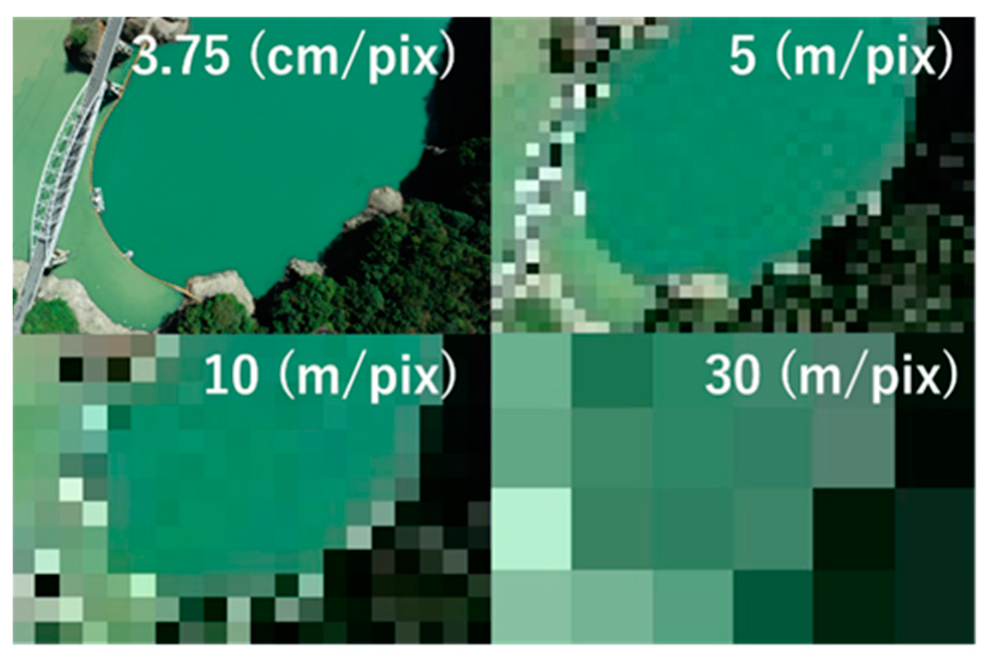
3.2. Turbidity Estimation from the Satellite Images

UAV aerial images have a higher spatial resolution than satellite images. In addition, as the shooting date is flexible, it does not necessarily coincide with the UAV aerial shooting date. However, since the flow in the lake is slow during fine days, turbidity changes are gentler than those in Chl-a. Considering this difference in the time progression speed, the WTI distribution obtained from the satellite images with a temporal gap of less than one week from the date of the aerial photography and no precipitation during that time can be used as a substitute for the turbidity distribution on the date of the aerial photography.

Figure 9 shows a correlation between the WTI and the measured turbidity at a depth of 1 m. Some points do not show a good correspondence. These are the results for the day when the bloom happened, and the point near the river inlet one month after the large-scale flood. As mentioned previously, when the bloom occurred, the dominant species near the surface layer were different from those in normal times, and it was assumed that the reflection characteristics were different from the normal condition, which also affected the turbidity evaluation results. In addition, near the river inlet after the flooding, dense turbid water was distributed in the deep layer, while the low-density clear water from the inflow river flowed into the surface layer. As a result, it was supposed that the color of the deep turbid water was transmitted through the shallow layer and appeared on the lake surface. Regarding these points, the relationship between the turbidity at a depth of 14 m and the WTI obtained from the profiler observation results is plotted again in the figure. The shifted marks show the same trend as the other results.

3.3. Classification of the Presence or Absence of Bloom and Regression of the Chl-a Concentration

The datasets without bloom (7 days) and with bloom (1 day: 16 July 2022) were used for the training and validation tests of the classification of the presence/absence of bloom. The bloom was visually confirmed on the aerial images, as shown in Figure 10. The test data were prepared from the datasets of two sampling points (50 sets) out of the five sampling points on the day of the bloom, and the other 50 sets were randomly selected from the data when the bloom did not occur. The other data (900 sets) were used as the training data.

Table 2. Confusion matrix of the classification of the presence/absence of bloom by XGBoost using the calibrated RGB, WTI, and water temperature as inputs.

	Predicted
	Presence	Absence
Presence	32	18
Absence	0	50

is the confusion matrix of the classification results. The total accuracy was 82%, the recall rate was 64%, and the precision rate was 100%. The false negative rate was high, but this is likely due to the use of the WTI as a parameter. The WTI can increase not only by the turbidity but also by the bloom, as mentioned above. For this reason, considerable “false negatives” might be found because it was not possible to classify cases when the bloom occurred and cases when the bloom did not occur but the turbidity was high.

Therefore, the WTI was omitted from the explanatory parameters for the classification of the presence or absence of bloom. The result using only the calibrated RGB reflectance and water temperature as the explanatory parameters is shown in

Table 3. Confusion matrix of the classification of the presence/absence of bloom by XGBoost using the calibrated RGB and water temperature as inputs.

	Predicted
	Presence	Absence
Presence	50	0
Absence	0	50

. By omitting the WTI, the presence/absence of bloom could be classified with a higher accuracy.

For the detection of the source of the nutrients contributing to blooms but before the occurrence of blooms, the distribution of a lower concentration of Chl-a is important information. The datasets of the days when the bloom did not occur were used for the regression of the Chl-a concentration. The explanatory parameters were the calibrated RGB, WTI, and temperature. All these parameters were normalized before the training and the validation. As discussed in the Introduction, in addition to Chl-a and the turbidity, CDOM is considered to be a factor that affects the water surface color. However, measuring CDOM is a heavy burden for practitioners in reservoir management, which undermines the main purpose of this study, that is, to develop a simple and flexible Chl-a monitoring method. However, the differentiation of absorption from phytoplankton and non-algal organic particles versus CDOM in surface waters is complex and challenging [60,61]. The reservoir of the study site has a comparatively high rotation of water and no specific resource of humic substances in the catchment area. Under such low-to-moderate levels of the humic color of water, there is only a small influence on the relationship between the Secchi disk transparency (SDT) and the Chl-a concentration, when the Chl-a levels are moderate or high [62]. Coelho et al. [63] showed that the range of variation in CDOM due to the reservoir operation is larger than its seasonal variation. Therefore, in the case of this study site, a reservoir under the influence with little inflow and outflow of humic substances, it is not necessary to consider the influence of CDOM when estimating the distribution of the Chl-a concentration. To simplify the focus of this study, we only included the WTI as the explanatory parameter of the water quality influencing the accuracy of the Chl-a evaluation.

In machine learning, success or failure depends on how the data are divided into test data and training data. Especially when the total amount of data is limited, as in this case, it affects the accuracy of evaluation results. We randomly selected two points (50 sets) from points A to E on each day as the test data, and three points (75 sets) as the training data. The coefficient of determination was 0.84, and reliable estimation accuracy was obtained in both cases. Figure 11 shows the correlation between the actual Chl-a concentrations and the estimated concentrations. Estimations can be made over a wide range from low to high concentrations, suggesting that it is possible to evaluate the Chl-a concentrations in the early stages of algae with lower concentrations from aerial images.

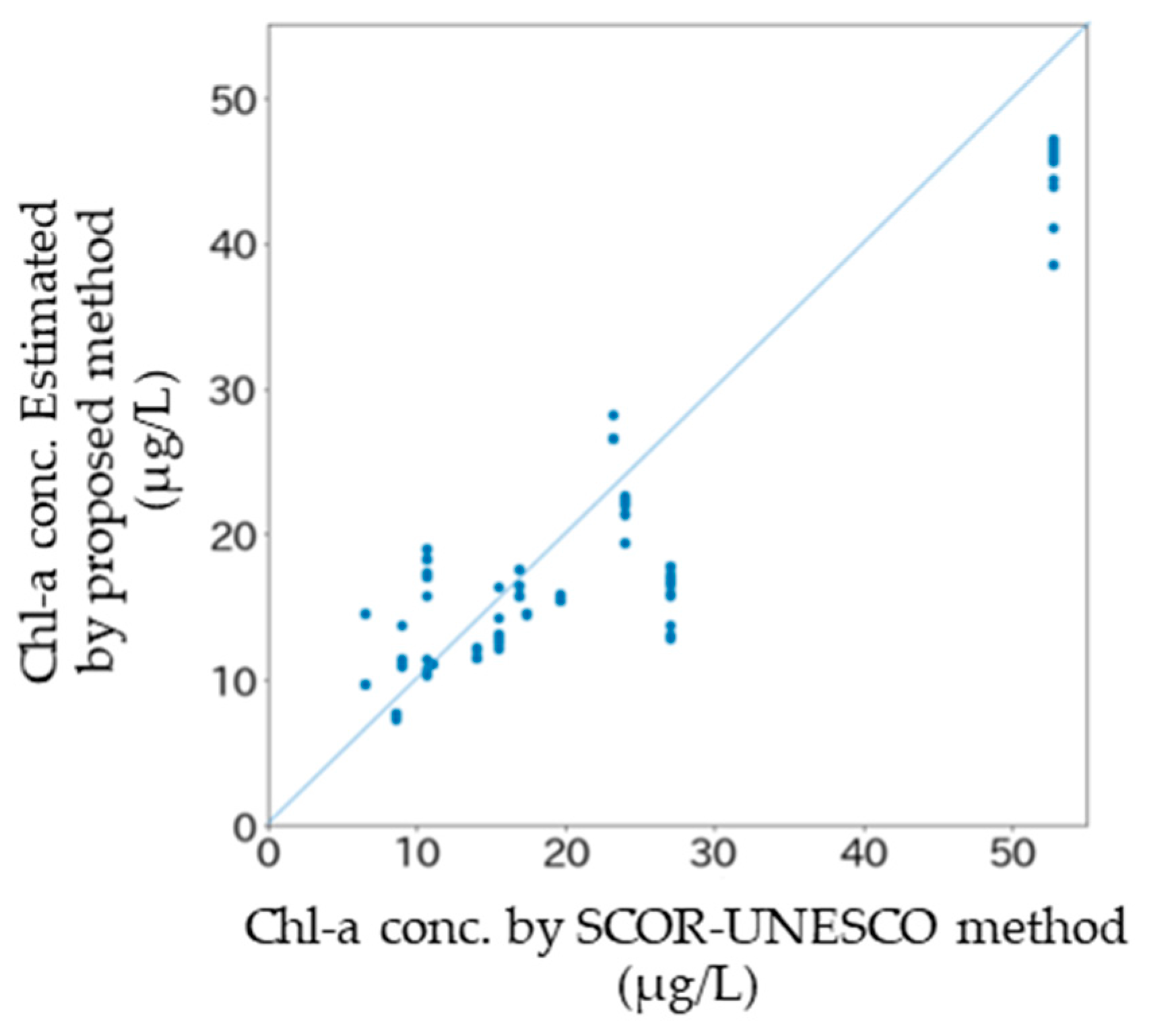
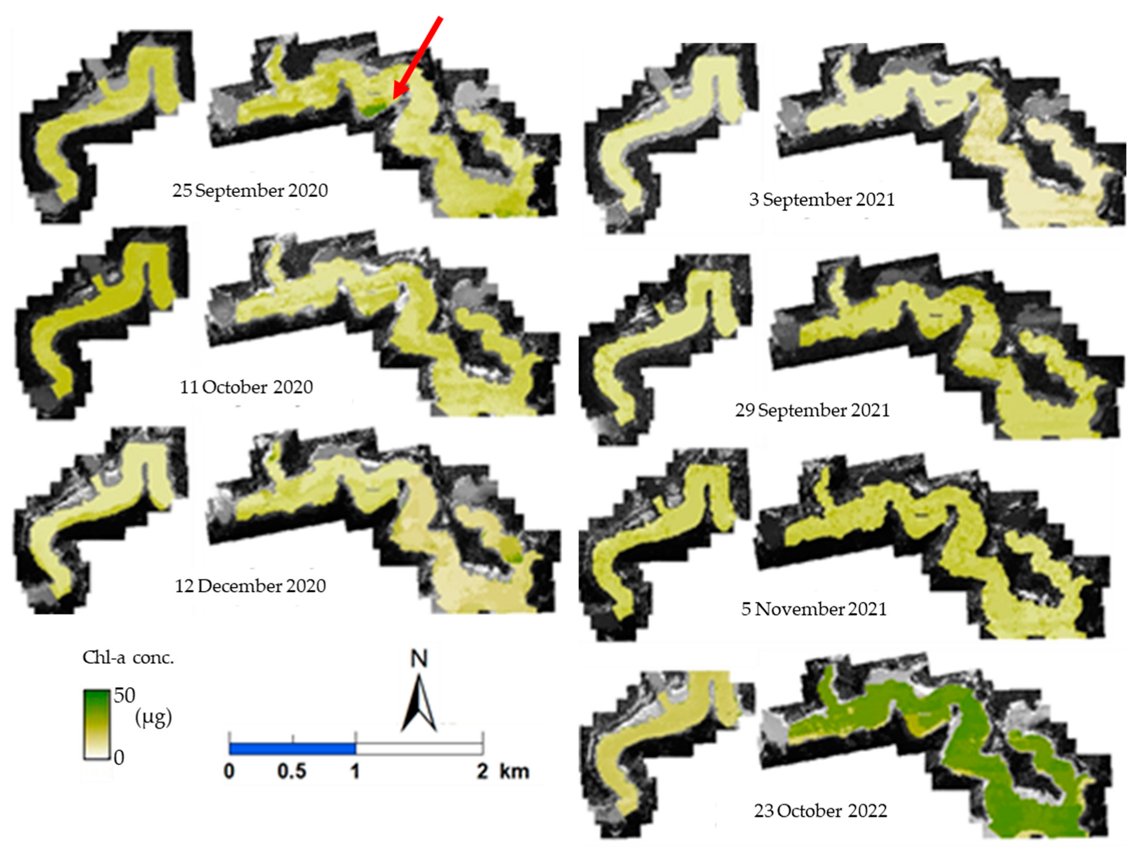
3.4. Distribution of the Concentration of Chl-a Estimated by the Proposed Method

Figure 12 shows the images before and after resizing. In the figure, GSD 10 m and 30 m images, which correspond to the resolution of the Sentinel and Landsat satellites, are also shown for comparison. Looking at Figure 12, it was thought that the Chl-a distribution could be sufficiently expressed with a GSD 5 m image. In addition, the hovering accuracy range of the UAV was ±0.5 m in the horizontal direction and ±1.5 m in the vertical direction, and it was thought that the error would become even larger due to the influence of the wind in the upper atmosphere. Therefore, even if we estimate the Chl-a concentration of each pixel by obtaining the luminance values at a resolution of 3.75 cm/pix, it is difficult to accurately project them onto a map. Therefore, in this study, we decided that a resolution of 5 m GSD was appropriate, considering the computational load also, and resized all images to be analyzed to a 5 m mesh using bilinear interpolation.

Figure 13 shows the distribution of the estimated Chl-a concentration on each observation date. No large spatial deviations were observed in the series of images from the same day, except in the case of 23 October 2022, when the largest flood happened one month before. It is known that, when such a large-scale outflow occurs in this reservoir, the turbid state differs depending on the inflowing river due to differences in the geological characteristics of the catchment area [55]. In this study, the WTI was included as an explanatory variable for machine learning. Therefore, from a negative perspective, it is possible that the high Chl-a concentration near the Shiromi River inflow area was due to a high WTI, and that the actual Chl-a concentration was not reproduced. However, in this study, as shown in Figure 11, the observation results with high WTI were included in the training of machine learning, and the test data in that area were well reproduced; so, the estimation accuracy was guaranteed.

On the other hand, it was confirmed that the concentration of Chl-a differed depending on the survey date. During normal times when there was little rainfall, such as in September and October 2020, the Chl-a concentration was slightly higher at the Hitotsuse River inlet. It is known that the Hitotsuse River basin has a relatively larger population and a slightly higher nutrient load than the Shiromi River basin. The results might reflect this difference in nutrient supply.

In the image of 25 September 2020, a small area with a high concentration indicated with the red arrow was found. This irregular distribution is due to the shade that is created by the neighboring mountain on the south side of the lake. Currently, there is no solution for such error induced by local shades, while the influence of the cloud cover change generally covers the survey area on the prediction of the Chl-a concentration.

4. Conclusions

Reservoirs located in mountainous areas are long and narrow in shape and have considerable inflow rivers, causing turbid water; so, there are many obstacles in understanding the spatial distribution of the chlorophyll-a concentration. In this study, we tried to estimate the distribution of chlorophyll-a by analyzing aerial images taken from UAVs, which have a high spatial resolution and a high flexibility of shooting schedule. The bloom of harmful algae is the most important event to control in reservoir management. However, in closed water bodies such as reservoirs with a limited surface area, the lake water is often completely eutrophic during the bloom stage. Furthermore, since floating harmful algae are blown by the wind, it is considered difficult to identify the source of nutrients from their spatial distribution. The proposed method provides the information of comparatively lower concentration of Chl-a than the bloom of the final stage of eutrophication so that it might contribute to finding a fundamental solution, such as the control of nutrient supply.

It was expected that the hue of the lake surface was determined by the turbidity discharged after flooding, in addition to the chlorophyll-a concentration. We calculated the WTI from satellite images and used it as one of the explanatory variables, together with the RGB values of aerial photographs to regression the chlorophyll-a concentration. The proposed method obtained good reproducibility. Turbid water behaves more slowly than chlorophyll, so even if there is a slight temporal gap between the date of aerial photography by the UAV and the day of shooting from satellites, the turbidity distribution does not change significantly. It will be possible to synchronize the evaluation of turbidity and spatial distribution of chlorophyll by equipping an UAV with a near-infrared camera [44], instead of using satellite images to evaluate the WTI. Since, likely, appropriate satellite images cannot be obtained due to weather conditions, it is desirable to obtain near-infrared reflectance using an UAV in the future to determine the WTI. In this study, turbidity was recognized as a factor that could affect the hue of the lake surface after a considerable number of observations had been completed; so, the monitoring with the UAV mounting a near-infrared sensor has not been conducted.

The chlorophyll-a concentrations evaluated by the proposed method were plotted on maps, which visually represented the temporal fluctuations in chlorophyll-a, and it was also possible to see that the chlorophyll-a concentrations differed depending on the inflowing rivers, even on the same day. However, the reflectance characteristics of chlorophyll and turbid water depend on the type of plankton that dominates and the geological characteristics of the basin. In particular, this study used a reservoir with a low inflow/outflow of CDOM as a research site and focused only on the effect of turbidity on the prediction accuracy of the chlorophyll-a concentration. So, to regress the chlorophyll-a concentration generally for any reservoir using a machine learning model, it is necessary to prepare learning data for each reservoir and build a model or to build a single model using images obtained from multiple reservoirs as training data. The results presented in this study are only based on the observations of the reservoir of our study site. This method might show limitations, for example, in that it is less suitable for reservoirs with a high flux of CDOM. For further study, it is necessary to improve the accuracy of the model by photographing and observing water quality in a lot of reservoirs, parallelly to challenge the differentiation of absorption from Chl-a and turbidity versus CDOM.

References

1. Ellison, M.E.; Brett, M.T. Particulate phosphorus bioavailability as a function of stream flow and land cover. Water Res. 2006, 40, 1258. [Google Scholar] [CrossRef] [PubMed]
2. Azhikodan, G.; Yokoyama, K. Spatio-temporal variability of phytoplankton (Chlorophyll-a) in relation to salinity, suspended sediment concentration, and light intensity in a macrotidal estuary. Cont. Shelf Res. 2016, 126, 15–26. [Google Scholar] [CrossRef]
3. Allison, A.O.; Randy, A.D.; Michae, L.D. The upside-down river: Reservoirs, algal blooms, and tributaries affect temporal and spatial patterns in nitrogen and phosphorus in the Klamath River, USA. J. Hydrol. 2014, 519, 164–176. [Google Scholar]
4. Dabrowski, T.; Lyons, K.; Nolan, G.; Berry, A.; Cusack, C.; Silke, J. Harmful algal bloom forecast system for SW Ireland. Part I: Description and validation of an operational forecasting model. Harmful Algae. 2016, 53, 64–76. [Google Scholar] [CrossRef] [PubMed]
5. Welch, E.B. Ecological Effects of Wastewater: Applied Limnology and Pollutant Effects, 2nd ed.; CRC Press: London, UK, 1992. [Google Scholar] [CrossRef]
6. Carmichael, W.W. The toxins of cyanobacteria. Sci. Am. 1994, 270, 78–84. [Google Scholar] [CrossRef] [PubMed]
7. Downing, J.A.; Watson, S.B.; McCauley, E. Predicting cyanobacteria dominance in lakes. Can. J. Fish. Aquat. Sci. 2001, 58, 1905–1908. [Google Scholar] [CrossRef]
8. Jilbert, T.; Couture, R.M.; Huser, B.J. Preface: Restoration of eutrophic lakes: Current practices and future challenges. Hydrobiologia 2020, 847, 4343–4357. [Google Scholar] [CrossRef]
9. Anderson, D.M.; Fensin, E.; Gobler, C.J.; Hoeglund, A.E.; Hubbard, K.A.; Kulis, D.M.; Landsberg, J.H.; Lefebvre, K.A.; Provoost, P.; Richlen, M.; et al. Marine harmful algal blooms (HABs) in the United States: History, current status and future trends. Harmful Algae 2021, 102, 101975. [Google Scholar] [CrossRef] [PubMed]
10. Anderson, D.M.; Cembella, A.D.; Hallegraeff, G.M. Progress in understanding harmful algal blooms: Paradigm shifts and new technologies for research, monitoring, and management. Annu. Rev. Mar. Sci. 2012, 4, 143–176. [Google Scholar] [CrossRef]
11. Díaz, P.A.; Ruiz-Villarreal, M.; Pazos, Y.; Moita, T.; Reguera, B. Climate variability and Dinophysis acuta blooms in an upwelling system. Harmful Algae 2016, 53, 145–159. [Google Scholar] [CrossRef]
12. Yu, Z.; Tang, Y.; Gobler, J.C. Harmful algal blooms in China: History, recent expansion, current status, and future prospects. Harmful Algae 2023, 129, 102499. [Google Scholar] [CrossRef] [PubMed]
13. Houliez, E.; Lizon, F.; Lefebvre, S.; Artigas, L.F.; Schmitt, F.G. Phytoplankton photosynthetic activity dynamics in a temperate macrotidal ecosystem (the Strait of Dover, eastern English Channel): Time scales of variability and environmental control. J. Mar. Syst. 2015, 147, 61–75. [Google Scholar] [CrossRef]
14. Azevedo, I.C.; Duarte, P.M.; Bordalo, A.A. Understanding spatial and temporal dynamics of key environmental characteristics in a mesotidal Atlantic estuary (Douro, NW Portugal). Estuar. Coast. Shelf Sci. 2008, 76, 620–633. [Google Scholar] [CrossRef]
15. Perry, R.I.; Nemcek, N.; Hennekes, M.; Sastri, A.; Ross, R.S.A.; Shannon, H.; Shartau, B.R. Domoic acid in Canadian Pacific waters, from 2016 to 2021, and relationships with physical and chemical conditions. Harmful Algae 2023, 129, 102530. [Google Scholar] [CrossRef] [PubMed]
16. Mori, M.; Gonzalez Flores, R.; Suzuki, Y.; Nukazawa, K.; Hiraoka, T.; Nonaka, H. Prediction of Microcystis Occurrences and Analysis Using Machine Learning in High-Dimension, Low-Sample-Size and Imbalanced Water Quality Data. Harmful Algae 2022, 117, 102273. [Google Scholar] [CrossRef] [PubMed]
17. Shan, K.; Wang, X.; Yang, H.; Zhou, B.; Song, L.; Shang, M. Use statistical machine learning to detect nutrient thresholds in Microcystis blooms and microcystin management. Harmful Algae 2020, 94, 101807. [Google Scholar] [CrossRef]
18. Wang, L.; Zhang, T.; Wang, X.; Jin, X.; Xu, J.; Yu, J.; Zhang, H.; Zhao, Z. An approach of improved Multivariate Timing-Random Deep Belief Net modeling for algal bloom prediction. Biosyst. Eng. 2019, 177, 130–138. [Google Scholar] [CrossRef]
19. Wang, F.; Guo, S.; Liang, J.; Sun, X. Water column stratification governs picophytoplankton community structure in the oligotrophic eastern Indian Ocean. Mar. Environ. Res. 2023, 189, 106074. [Google Scholar] [CrossRef] [PubMed]
20. Jiang, Y.J.; He, W.; Liu, W.X.; Qin, N. The seasonal and spatial variations of phytoplankton community and their correlation with environmental factors in a large eutrophic Chinese lake (Lake Chaohu). Ecol. Indic. 2014, 40, 58–67. [Google Scholar] [CrossRef]
21. Dale, B.; Murphy, M. A retrospective appraisal of the importance of high-resolution sampling for harmful algal blooms: Lessons from long-term phytoplankton monitoring at Sherkin Island, S.W. Ireland. Harmful Algae 2014, 40, 23–33. [Google Scholar] [CrossRef]
22. Nwe, L.W.; Yokoyama, K.; Azhikodan, G. Phytoplankton habitats and size distribution during a neap-spring transition in the highly turbid macrotidal Chikugo River estuary. Sci. Total Environ. 2022, 850, 157810. [Google Scholar] [CrossRef] [PubMed]
23. Chaffin, J.D.; Kane, D.D.; Stanislawczyk, K.; Parker, E.M. Accuracy of data buoys for measurement of cyanobacteria, chlorophyll, and turbidity in a large lake (Lake Erie, North America): Implications for estimation of cyanobacterial bloom parameters from water quality sonde measurements. Environ. Sci. Pollut. Res. Int. 2018, 25, 25175–25189. [Google Scholar] [CrossRef] [PubMed]
24. Veerapaga, N.; Shintani, T.; Azhikodan, G.; Yokoyama, K. Study on Salinity Intrusion and Mixing Types in a Conceptual Estuary Using 3-D Hydrodynamic Simulation: Effects of Length, Width, Depth, and Bathymetry. In Estuaries and Coastal Zones in Times of Global Change; Nguyen, K., Guillou, S., Gourbesville, P., Thiébot, J., Eds.; Springer: Singapore, 2020. [Google Scholar] [CrossRef]
25. Nakayama, K.; Komai, K.; Amano, M.; Horii, S.; Somiya, Y.; Kumamoto, E.; Oyama, Y. Ideal water temperature environment for giant Marimo (Aegagropila linnaei) in Lake Akan, Japan. Sci. Rep. 2023, 13, 16834. [Google Scholar] [CrossRef] [PubMed]
26. Le, H.N.; Shintani, T.; Nakayama, K. A Detailed Analysis on Hydrodynamic Response of a Highly Stratified Lake to Spatio-Temporally Varying Wind Field. Water 2023, 15, 565. [Google Scholar] [CrossRef]
27. Xu, X.; Ishikawa, T.; Nakamura, T. Three-dimensional modeling of hydrodynamics and dissolved oxygen transport in tone river estuary. J. JSCE 2013, 1, 194–213. [Google Scholar] [CrossRef] [PubMed]
28. Huang, J.; Zhang, Y.; Huang, Q.; Gao, J. When and where to reduce nutrients for controlling harmful algal blooms in large eutrophic lake Chaohu, China? Ecol. Indic. 2018, 89, 808–817. [Google Scholar] [CrossRef]
29. Maguire, J.; Cusack, C.; Ruiz-Villarreal, M.; Silke, J.; McElligott, D.; Davidson, K. Applied simulations and integrated modeling for the understanding of toxic and harmful algal blooms (ASIMUTH): Integrated HAB forecast systems for Europe’s Atlantic Arc. Harmful Algae 2016, 53, 160–166. [Google Scholar] [CrossRef] [PubMed]
30. Lin, Z.; Zhan, P.; Li, J.; Sasaki, J.; Qiu, Z.; Chen, C.; Zou, S.; Yang, X.; Gu, H. Physical drivers of Noctiluca scintillans (Dinophyceae) blooms outbreak in the northern Taiwan Strait: A numerical study. Harmful Algae 2024, 133, 102586. [Google Scholar] [CrossRef] [PubMed]
31. Jin, D.; Lee, E.; Kwon, K.; Kim, T. A deep learning model using satellite ocean color and hydrodynamic model to estimate chlorophyll-a concentration. Remote Sens. 2021, 13, 2003. [Google Scholar] [CrossRef]
32. Mamun, M.; Ferdous, J.; An, K.-G. Empirical estimation of nutrient, organic matter and algal chlorophyll in a drinking water reservoir using Landsat 5 TM data. Remote Sens. 2021, 13, 2256. [Google Scholar] [CrossRef]
33. Li, D.; Gao, Z.; Song, D.; Shang, W.; Jiang, X. Characteristics and influence of green tide drift and dissipation in Shandong Rongcheng coastal water based on remote sensing. Estuar. Coast. Shelf Sci. 2019, 227, 106335. [Google Scholar] [CrossRef]
34. Hu, L.; Zeng, K.; Hu, C.; He, M.X. On the remote estimation of Ulva prolifera areal coverage and biomass. Remote Sens. Environ. 2019, 223, 194–207. [Google Scholar] [CrossRef]
35. Mugani, R.; El Khalloufi, F.; Kasada, M.; Redouane, M.; Haida, M.; Aba, R.P.; Essadki, Y.; Zerrifi, S.A.; Herter, S.O.; Hejjaj, A.; et al. Monitoring of toxic cyanobacterial blooms in Lalla Takerkoust reservoir by satellite imagery and microcystin transfer to surrounding farms. Harmful Algae 2024, 135, 102631. [Google Scholar] [CrossRef]
36. Chen, X.; Shang, S.; Lee, Z.; Qi, L.; Yan, J.; Li, Y. High-frequency observation of floating algae from AHI on Himawari-8. Remote Sens. Environ. 2019, 227, 151–161. [Google Scholar] [CrossRef]
37. Liu, M.; Ling, H.; Wu, D.; Su, X.; Cao, Z. Sentinel-2 and Landsat-8 Observations for Harmful Algae Blooms in a Small Eutrophic Lake. Remote Sens. 2021, 13, 4479. [Google Scholar] [CrossRef]
38. Ma, J.; Jin, S.; Li, J.; He, Y.; Shang, W. Spatio-Temporal Variations and Driving Forces of Harmful Algal Blooms in Chaohu Lake: A Multi-Source Remote Sensing Approach. Remote Sens. 2021, 13, 427. [Google Scholar] [CrossRef]
39. Zhang, T.; Hu, H.; Ma, X.; Zhang, Y. Long-Term Spatiotemporal Variation and Environmental Driving Forces Analyses of Algal Blooms in Taihu Lake Based on Multi-Source Satellite and Land Observations. Water 2020, 12, 1035. [Google Scholar] [CrossRef]
40. Soomets, T.; Uudeberg, K.; Jakovels, D.; Brauns, A.; Zagars, M.; Kutser, T. Validation and Comparison of Water Quality Products in Baltic Lakes Using Sentinel-2 MSI and Sentinel-3 OLCI Data. Sensors 2020, 20, 742. [Google Scholar] [CrossRef] [PubMed]
41. Toth, C.; Jóźków, G. Remote sensing platforms and sensors: A survey. ISPRS J. Photogramm. Remote Sens. 2016, 115, 22–36. [Google Scholar] [CrossRef]
42. Vélez-Nicolás, M.; García-López, S.; Barbero, L.; Ruiz-Ortiz, V.; Sánchez-Bellón, Á. Applications of unmanned aerial systems (UASs) in hydrology: A review. Remote Sens. 2021, 13, 1359. [Google Scholar] [CrossRef]
43. Qu, M.; Anderson, S.; Lyu, P.; Malang, Y.; Lai, J.; Liu, J.; Jiang, B.; Xie, F.; Liu, H.H.; Lefebvre, D.D.; et al. Effective aerial monitoring of cyanobacterial harmful algal blooms is dependent on understanding cellular migration. Harmful Algae 2019, 87, 101620. [Google Scholar] [CrossRef] [PubMed]
44. Guimarães, T.T.; Veronez, M.R.; Koste, E.C.; Gonzaga, L.; Bordin, F.; Inocencio, L.C.; Larocca, A.P.C.; De Oliveira, M.Z.; Vitti, D.C.; Mauad, F.F. An Alternative Method of Spatial Autocorrelation for Chlorophyll Detection in Water Bodies Using Remote Sensing. Sustainability 2017, 9, 416. [Google Scholar] [CrossRef]
45. Su, T.-C.; Chou, H.-T. Application of Multispectral Sensors Carried on Unmanned Aerial Vehicle (UAV) to Trophic State Mapping of Small Reservoirs: A Case Study of Tain-Pu Reservoir in Kinmen, Taiwan. Remote Sens. 2015, 7, 10078–10097. [Google Scholar] [CrossRef]
46. Cheng, K.H.; Chan, S.N.; Lee, J.H.W. Remote sensing of coastal algal blooms using unmanned aerial vehicles (UAVs). Mar. Pollut. Bull. 2020, 152, 110889. [Google Scholar] [CrossRef]
47. Cao, Z.; Duan, H.; Feng, L.; Ma, R.; Xue, K. Climate- and human-induced changes in suspended particulate matter over Lake Hongze on short and long timescales. Remote Sens. Environ. 2017, 192, 98–113. [Google Scholar] [CrossRef]
48. Hu, C.; Chen, Z.; Clayton, T.D.; Swarzenski, P.; Brock, J.C.; Muller–Karger, F.E. Assessment of estuarine water-quality indicators using MODIS medium-resolution bands: Initial results from Tampa Bay, FL. Remote Sens. Environ. 2004, 93, 423–441. [Google Scholar] [CrossRef]
49. Kishino, M.; Tanaka, A.; Ishizaka, J. Retrieval of Chlorophyll a, suspended solids, and colored dissolved organic matter in Tokyo Bay using ASTER data. Remote Sens. Environ. 2005, 99, 66–74. [Google Scholar] [CrossRef]
50. Sakuno, Y.; Yajima, H.; Yoshioka, Y.; Sugahara, S.; Abd Elbasit, M.A.M.; Adam, E.; Chirima, J.G. Evaluation of Unified Algorithms for Remote Sensing of Chlorophyll-a and Turbidity in Lake Shinji and Lake Nakaumi of Japan and the Vaal Dam Reservoir of South Africa under Eutrophic and Ultra-Turbid Conditions. Water 2018, 10, 618. [Google Scholar] [CrossRef]
51. Palmer, S.C.J.; Hunter, P.D.; Lankester, T.; Hubbard, S.; Spyrakos, E.N.; Tyler, A.; Présing, M.; Horváth, H.; Lamb, A.; Balzter, H.; et al. Validation of Envisat MERIS algorithms for chlorophyll retrieval in a large, turbid and optically-complex shallow lake. Remote Sens. Environ. 2015, 157, 158–169. [Google Scholar] [CrossRef]
52. Alcântara, E.; Bernardo, N.; Watanabe, F.; Rodrigues, T.; Rotta, L.; Carmo, A.; Shimabukuro, M.; Gonçalves, S.; Imai, N. Estimating the CDOM absorption coefficient in tropical inland waters using OLI/Landsat-8 images. Remote Sens. Lett. 2016, 7, 661–670. [Google Scholar] [CrossRef]
53. Glukhovets, D.; Kopelevich, O.; Yushmanova, A.; Vazyulya, S.; Sheberstov, S.; Karalli, P.; Sahling, I. Evaluation of the CDOM absorption coefficient in the Arctic seas based on Sentinel-3 OLCI data. Remote Sens. 2020, 12, 3210. [Google Scholar] [CrossRef]
54. Yamagata, Y.; Wiegand, C.; Akiyama, T.; Shibayama, M. Water turbidity and perpendicular vegetation indices for paddy rice flood damage analyses. Remote Sens. Environ. 1988, 26, 241–251. [Google Scholar] [CrossRef]
55. Murakami, T.; Suzuki, Y.; Oishi, H.; Ito, K.; Nakao, T. Tracing the source of difficult to settle fine particles which cause turbidity in the Hitotsuse reservoir. J. Environ. Manag. 2013, 120, 37–47. (In Japanese) [Google Scholar] [CrossRef]
56. Murakami, T.; Nakayama, H.; Mizuguchi, S.; Sugio, S.; Ootawara, N. Effective Countermeasures to long-term Turbid Water Effluence from the Hitotsuse Dam Reservoir. In Environmental Hydraulics, Two Volume Set; CRC Press: Athens, Greece, 2010; pp. 23–25. [Google Scholar] [CrossRef]
57. Chen, T.; Guestrin, C. XGBoost: A Scalable Tree Boosting System. In Proceedings of the KDD’16: 22nd ACM SIGKDD International Conference on Knowledge Discovery and Data Mining, San Francisco, CA, USA, 13–17 August 2016. [Google Scholar]
58. Available online: https://microsoft-image-composite-editor-64bits.en.softonic.com/?ex=RAMP-1768.3 (accessed on 4 April 2024).
59. Irie, M.; Arakaki, S.; Suto, T.; Umino, T. Classification of River Sediment Fractions in a River Segment including Shallow Water Areas Based on Aerial Images from Unmanned Aerial Vehicles with Convolution Neural Networks. Remote Sens. 2024, 16, 173. [Google Scholar] [CrossRef]
60. Brezonik, P.L.; Olmanson, L.G.; Finlay, J.C.; Bauer, M.E. Factors affecting the measurement of CDOM by remote sensing of optically complex inland waters. Remote Sens. Environ. 2015, 157, 199–215. [Google Scholar] [CrossRef]
61. Shao, T.; Song, K.; Du, J.; Zhao, Y.; Lui, Z.; Zhang, B. Retrieval of CDOM and DOC using in situ hyperspectral data: A case study for potable water in Northeast China. J. Indian Soc. Remote Sens. 2015, 44, 77–89. [Google Scholar] [CrossRef]
62. Brezonik, P.; Menken, K.D.; Bauer, M. Landsat-based remote sensing of lake water quality characteristics, including chlorophyll and colored dissolved organic matter (CDOM). Lake Reserv. Manag. 2005, 21, 373–382. [Google Scholar] [CrossRef]
63. Coelho, C.; Heim, B.; Foerster, S.; Brosinsky, A.; De Araújo, J.C. In Situ and Satellite Observation of CDOM and Chlorophyll-a Dynamics in Small Water Surface Reservoirs in the Brazilian Semiarid Region. Water 2017, 9, 913. [Google Scholar] [CrossRef]
Figure 1. Location of the Hlitotsuse Reservoir (Lake Mera) and the Photographed area. Blue area: lake surface, red area: photographed from UAV, reverse triangle: water sampling points.
Drones 08 00224 g001
Figure 2. Shooting settings.
Drones 08 00224 g002
Figure 3. Correlation between the fluorescence intensity of the Uranine concentration reference and the concentration of Chl-a by the COR-UNESCO method.
Drones 08 00224 g003
Figure 4. Water temperature (bars) and turbidity (marks) of the water at a 1 m depth at the profiling points.
Drones 08 00224 g004
Figure 5. Flow chart of the classification of the presence/absence of bloom and the regression of the concentration of Chl-a. WTI was used as input parameter in the first attempt of the classification. Due to the low accuracy of that result, it was omitted from the input parameter in the second attempt. Then, WTI was included in the stage of the repression of Chl-a concentration.
Drones 08 00224 g005
Figure 6. Photographs of the same area at different times within the same day and fluctuations in insolation. (au) indicate the time in the right figures showing the fluctuation of the insolation.
Drones 08 00224 g006
Figure 7. Relationship between the insolation intensity and calibration coefficients.
Drones 08 00224 g007
Figure 8. Reflectance calibration for the images taken in during a fight based on insolation. (Left): Before the calibration.; (Right): After the calibration. The area surrounded by the red break line was photographed when the insolation was extremely low by cloud.
Drones 08 00224 g008
Figure 9. Correlation between the turbidity measured from A to E on each observation date. And the WTI calculated from the satellite image. Colors indicate the dates and the shapes indicate the locations.
Drones 08 00224 g009
Figure 10. Aerial photograph when the bloom was present.
Drones 08 00224 g010
Figure 11. Comparison between the true and estimated Chl-a concentrations.
Drones 08 00224 g011
Figure 12. Images resized with different resolutions.
Drones 08 00224 g012
Figure 13. Distribution of the estimated Chl-a concentration on each observation date. Red arrow on the top left image is pointing the area indicating the high concentration due to the shade that is created by the neighboring mountain.
Drones 08 00224 g013