Safety and Security-Specific Application of Multiple Drone Sensors at Movement Areas of an Aerodrome

Abstract

Nowadays, the public service practice applicability of drones and remote sensing sensors is being explored in almost all industrial and military areas. In the present research, in collaboration with different universities, we investigate the applicability of drones in airport procedures, assessing the various potential applications. By exploiting the data from remote sensing sensors, we aim to develop methodologies that can assist airport operations, including managing the risk of wildlife threats to runway safety, infrastructure maintenance, and foreign object debris (FOD) detection. Drones equipped with remote sensing sensors provide valuable insight into surface diagnostics, helping to assess aprons, taxiways, and runways. In addition, drones can enhance airport security with effective surveillance and threat detection capabilities, as well as provide data to support existing air traffic control models and systems. In this paper, we aim to present our experience with the potential airport applications of UAV high-resolution RGB, thermal, and LiDAR sensors. Through interdisciplinary collaboration and innovative methodologies, our research aims to revolutionize airport operations, safety, and security protocols, outlining a path toward a safer, more efficient airport ecosystem.

1. Introduction

The drone industry has experienced explosive development, which is addressing technical, regulatory, control, and safety issues. The market for drones and their applications is constantly growing; their use raises new questions and requires new approaches [1,2,3,4,5,6]. Their application creates new opportunities for industrial [7,8], agricultural [9,10,11,12,13], wildlife detection [14,15,16,17], research [18,19,20,21], public service [22,23,24,25], and defense applications [26,27].

Today, the airport, which is one of the most complex infrastructures in aviation, is still strictly protected from drone flights. But it is clear that the potential of the technology will allow unmanned aerial vehicles (UAV) to use airports within a few years (SORA analysis in Luxemburg airport [28,29]: at Luxemburg Airport, a drone operation was carried out, and according to European Union regulation, it was a “specific” category operation. For a “specific” category operation, it is mandatory to carry out a safety assessment. Operators chose “Specific Operations Risk Assessment”, which is a risk analysis procedure). Furthermore, the appearance of various small-scale drones at airports use camera and remote sensing sensor data, mainly for safety and security purposes.

The ‘Integrated Model Airport’ (hereinafter IMA) research, which has been running since 2022 in the aviation departments of the University of Public Service ‘Ludovika’, focuses on exploring the possibilities of piloted and unmanned aircraft operating together at the airport. One of our objectives is to survey what procedures are taken in force, within what time slots, and for what tasks drones can be integrated into the daily traffic flow of the airport. The purpose of the cooperation between researchers of the Eötvös Loránd University and University of Public Service Ludovika is to gain experience in different use cases of drones carrying out airport tasks, to demonstrate their effect on daily operations, as well as to collect data through remote sensing and other in situ spatial information measurements.

The data and traffic of the IMA are based on existing conditions in LHSN (Szolnok, Hungary), which is primarily open to military traffic.

The airport traffic generally follows the rules known from international standards; however, a range of special regulations are in force, supervised by the military aviation authority (hereafter MAA). The airspace structure of the airport and the surrounding and neighboring airspaces are complex [30,31] and do not favor drone flights due to the closure of critical infrastructure, nature reserves, non-towered airfields, and a medical heliport. The airport almost grew together with the city and several residential areas are located nearby. A concept of operation (ConOps) was established by our team before the flight operation. In this so-called ConOps, several factors were taken into account such as Ground Risk and Air Risk. According to European [32,33] and national regulations [34], the majority of the airport maneuvering area is protected by a no-drone zone [31], which serves to keep civil drones away and save manned flights from interactions with UAVs and mid-air collisions. The planned operation looked impossible because most of the commercial drones are pre-programmed to avoid the aforementioned areas. Nevertheless, this dual regulatory environment (military/civil) may provide an extensive basis for drone operations at airports. According to our hypothesis, the gained experience in the organization and operation of drone flights will provide us with a comprehensive view and take into account administrative challenges and potential benefits.

The airport is also interesting in terms of its environmental location and has plenty of wildlife risk. To maintain bird control and reduce wildlife risk, it is essential to control rodent numbers, the first stage of which is a thorough survey and mapping. One of today’s emerging technologies is the evaluation of data from drone-based imagery for agricultural purposes, which in this case can be a useful tool for mapping rodent populations. This information can take wildlife control to a more professional level.

The various remote sensing sensors (e.g., spectral, thermal, photogrammetric, or LiDAR sensors) installed on today’s modern drones also provide the possibility to assess the condition of aprons, taxiways, and runways, to monitor cracks in solid surfaces. More international studies deal with the applicability of these sensors for surface diagnostics. Spectral, visible, and thermal imaging is suitable for examining surface deformation, disintegration, and cracking damage, as well as moisture-related analyses. The LiDAR sensor, in addition to the former, can also carry out subsidence and sinkhole damage tests [35,36,37,38]. One of the aims of our experiment is to set up a reference database to make preplanned maintenance work more effectively. According to our assumptions, there has been no such research carried out or any reference database created in Hungary before, especially at military airports.

The survey described above can also assist in the detection of Foreign Object Debris (FOD). FOD could be any item that is found at the airside of the airport and could cause damage to the aircraft and injury to personnel. Airside covers that area of the airport where aircraft can safely move and park. A range of different objects can be FOD regardless of material, such as debris, any contaminations, cans, abandoned tools, pieces of luggage, rocks, and even mortal remains of wildlife [39].

The above-listed use cases serve safety purposes, but drones can be effective in the security chain of the airport. Drones’ ability to quickly change position enables them to inspect large areas in a relatively short time or to conduct rapid ad hoc searches over a defined area. Thanks to the various camera sensors mounted on drones, high-resolution live images are provided through data links day and night, and, with the usage of artificial intelligence, these images can greatly facilitate threat detection and ultimately reduce the need for human resources.

The most important questions of this research are whether it is worth using work drones at the airport, for what purpose, and with what sensors. Airports are “no-drone zones” for a reason, but it is worth examining where the boundaries can be drawn in the issue of aviation safety versus innovation. The use of drones for this purpose can even support flight safety because, depending on the season or time of the day, the properly selected sensors are more likely to find, e.g., foreign objects than the current process of using human resources and vehicles.

Our long-term goal is to develop a complex flight strategy (with the ideal flight altitude and fastest, most energy-saving flight path), which can be used for airport security on a daily basis. The first step—which this manuscript is also about—was to select the most useful sensor(s) for certain assigned tasks. In this case, FOD and small mammal detection in any season with the expected accuracy.

2. Materials and Methods

2.1. Study Area

The location was the LHSN airport in Szolnok, Hungary (Figure 1). The total surveyed area (Aerodrome Reference Point (ARP) coordinates: Lat = N 47°07′22″, Lon = E 20°14′08″) was 17.835 ha. The field study was carried out on 8–10 December 2023. As mentioned previously, the airport is mainly used by numerous helicopters and small aircraft on a daily basis. Although aircraft accommodated at the airport are mainly small sized, e.g., two-seater trainer aircraft (ZLIN142) and helicopters (H145, H225), the traffic peaks close to medium-sized airports on weekdays [40,41,42]. This is because the airport serves a number of flight missions and training tasks. Moreover, it is the home base of the search and rescue service, which is why an experimental real drone flight can only be carried out during a non-flying weekend.

The location of the airport and its environment accompanies a range of wildlife risks. At the northern part of the airport, there is a pond, named Holt-Tisza, which has a large-scale water surface with a significant waterfowl population, affecting the approach path and climbing areas of the runway. At the eastern part of the airport, a neighboring farmland is located and serves as a feeding chamber for rodents. Because of significant rodent presence, many uphill warehouses had increased rodent populations, and hollows were dug under the surface of the movement area. The spread of the rodent population attracts birds of prey. In order to control the numbers of birds and reduce wildlife risk, it is necessary to determine rodent-polluted areas through mapping and a drone-observed survey. Ranges of emerging technologies support the evaluation of data, drone-based imagery for agricultural purposes, in this case for mapping the rodent population. This information can take bird control to a more professional level.

2.2. Used Equipment

The field study was carried out with a DJI Matrice 350 RTK drone (due to its comparatively greater mass it can be used to lift a wide variety of sensors, which was cardinal from the point of view of the research) equipped with a Zenmuse P1 RGB camera, a Zenmuse L1 LiDAR sensor, and a Zenmuse H20T thermal camera. The almost same examined area was recorded separately with all three sensors (Figure 2).

The DJI Matrice 350 RTK drone has a quadcopter design, which can reach a flight duration of up to 55 min, and it can also carry a maximum of 2.7 kg of extra weight. Thanks to the intelligent battery charging system of the new generation BS65, it speeds up the recharging of the batteries [43]. The RTK GPS (Real-Time Kinematic) provides real-time three-dimensional positioning results of the station in the specified coordinate system and can achieve centimeter-level accuracy. During the survey, 3 pairs of batteries (6 pieces in total) were prepared, which were continuously recharged during the day.

The Zenmuse L1 LiDAR sensor is a dual camera, with a maximum of three signal return-supported LiDAR sensors and a high-resolution RGB camera [44]. The LiDAR sensor’s ranging accuracy arrives at 3 cm from 100 m height/altitude. Its point rate arrives at the max. 240,000 pts/s (single mode) or the max. 480,000 pts/s (multiple return mode). Its detection range should arrive at 450 m. In scanning mode, it supports the repetitive and the non-repetitive mode too. For point cloud coloring, the reflectivity, height, distance, or RGB values can be selected as basic parameters. The highest accuracy is achieved in suitable light conditions and near-optimal flight speed. The standard file formats for LiDAR point clouds are .las or .laz. However, the DJI Zenmuse L1 uses a closed data format, so for data processing the DJI Terra software (V4.0.10) was needed to prepare or convert the results into a .las point cloud. The software also enables some measurements and the creation of specific models (e.g., DSM), but it cannot perform the classification of the point cloud.

Zenmuse H20T dual thermal camera has a built-in high-resolution 20 MP RGB camera [45]. The thermal camera arrives at 640 × 512 px resolution, its digital zoom can max 8x. Thanks to the dual camera, the resolution of the thermal data can be improved with the help of the high-resolution RGB image, with the so-called pansharpening interpolation procedure. The spectral sensibility of the thermal camera based on the microbolometer principle is in the 8–14 μm spectral range. An 85% image overlap is recommended during recording/capturing. Its image format is 16-bit .R-JPG (radiometric JPG) or .T-JPG (thermal JPG).

DJI Zenmuse P1 is a 45 MP high-resolution, full-frame RGB camera, designed for photogrammetry flight missions [46]. Without any GCP points its accuracy can reach 3 cm horizontally and 5 cm vertically, if we take care when capturing to fix the 75% front and 55% side overlap rate. Its pixel size is 4.4 µm and it can take a photo every 0.7 s. Its photo size is 8192 × 5460 px resolution. The flight speed should be chosen according to the application scenario, as it may affect the quality. Regarding mission mode, a 2D orthomosaic mission, 3D oblique mission, detailed modeling mission, or real-time mapping mission can be chosen.

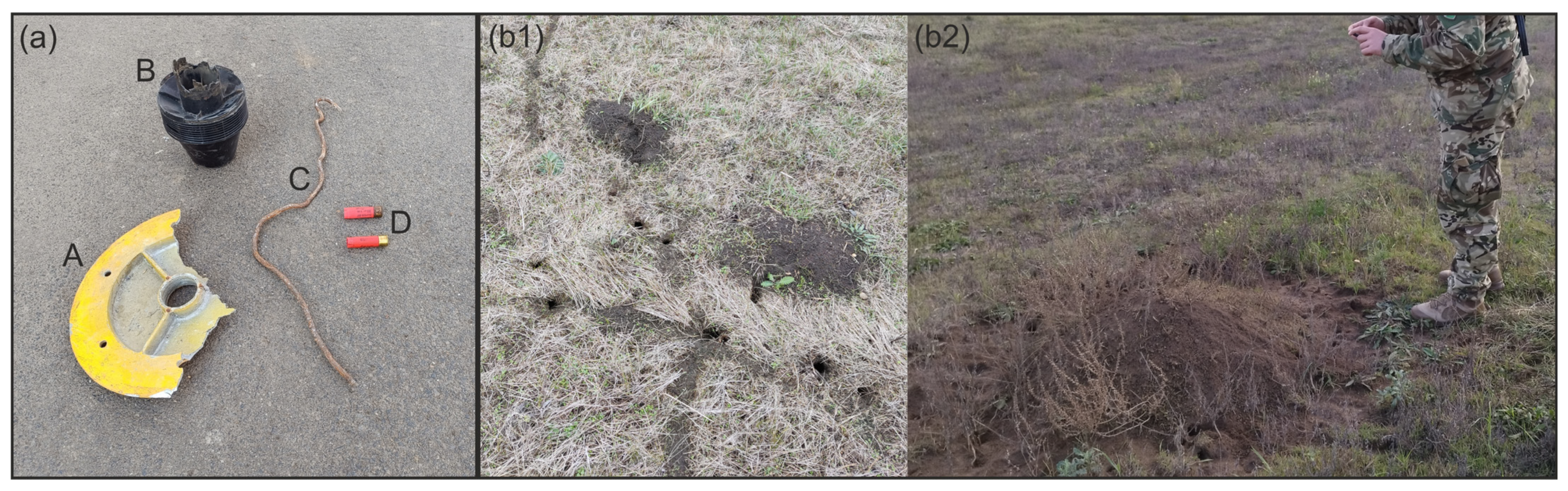
For FOD detection, four objects were put on the runway (Figure 3a), and next to the runway, there are plenty of field-vole holes (bigger hill in b2, smaller with holes and routes in b1). When choosing the flight area, the following aspects were taken into account: the bases were the selected FOD and the sensitive areas of the runway, such as the “touch-down zones”, the vicinity of the most frequently used taxiways, and the areas where the decision speed is reached.

During the FOD selection process, the following criteria were considered: they were made from various materials (A (side light lamp subframe), C (wire) metal or metallic alloy, B (tractor engine air filter) plastic, D (shotgun cartridge case) mixed), their shapes varied (whereas A, B, D can be considered regular, enclosed bodies, C is irregular, with a thin linear form), and in terms of color, two differed from the surface (A—yellowish, D—red) while two were of similar shade to the surface (C—light gray, B—dark gray). The sizes of the FOD can be seen in

Table 1. The extent of the FOD.

FOD Size (mm)	Length (x)	Width (y)	Height (z)
A	335	240	35
B	160	160	210
C	675	10	10
D	65	20	23

:

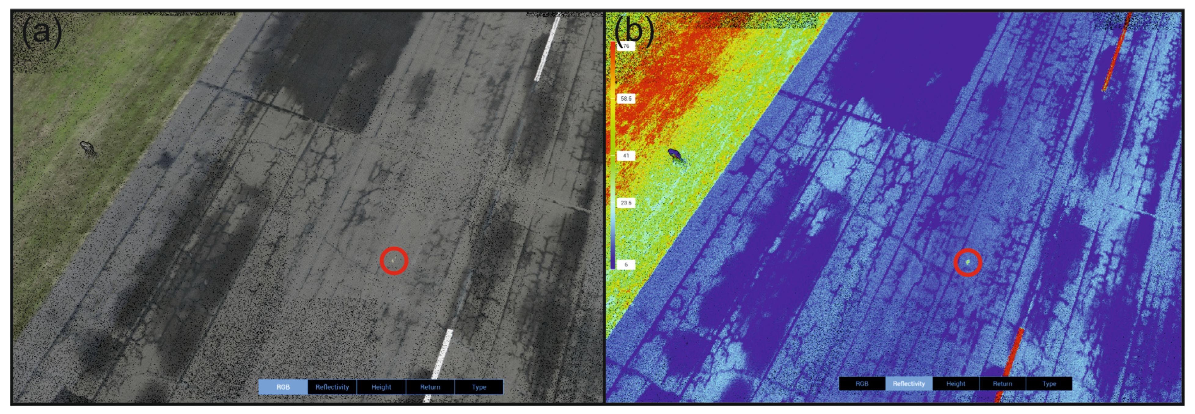
Due to the weather conditions, the first measurement was carried out with the LiDAR sensor in an effort to improve lighting conditions. The study area was recorded with two battery replacements (DJI TB65 Lithium-ion battery: 5880 mAh/piece; they must be used in pairs for one flight and they can be replaced one at a time so the running program is not interrupted, nor does the sensor require recalibration). The flight was performed with the Ground Sampling Distance (GSD) value set, so the flight altitude and speed were calculated by the system at an altitude of 30 m. The resulting image reached a resolution of under 1 cm, which was necessary to meet research purposes.

The second flight was carried out equipped with the H20T thermal sensor. Targeting the same GSD value, the system calculated a flight height of 50 m. In addition, due to the 85% image overlap, the duration would have been more than 10 h. Because of this, we overrode the flight parameter and flew at a height of 50 m with two battery replacements, thus reaching GSD ~5 cm.

The third flight was carried out equipped with the P1 sensor. Targeting the same GSD value, the system calculated a flight height of 50 m, with a 5.1 ms⁻¹ flight speed.

The main characteristics of the data captured by the three sensor systems can be seen in

Table 2. The main characteristics of the data captured by the three sensor systems.

Sensor	GSD (cm/pixel)	Altitude (m)	Speed (m/s)	Number of Pictures
L1	0.83	30	3.5	736
H20T	4.44	50	3	2227
P1	0.63	50	5.1	968

.

2.3. Legal Background

As the examined area is in Hungary, it is necessary to give some overview of the actual legal background of drone operations.

For a legal flight of drones before takeoff, it is necessary to register (1) the drone, and (2) the pilot (operator). After the registration, the authority gives an ID that must be placed on the drone in a visible part. The operator must have insurance and a valid EASA pilot license (see details in [47,48]). After having the above-mentioned documents, the “pre-flight” preparations can be started: in every case, to use controlled airspace, permission is needed. It is namely an ad hoc segregated area. It can be booked for 7 days, a minimum of 30 days before the planned flight. If the airspace is somehow special (e.g., nature reserve, around heliports/airports), this administration period can take more time. Before starting the specific flight, the use of a mobile application MyDroneSpace is mandatory as the experimental flight remained in a visual line-of-sight area that does not exceed ‘open’ category criteria according to Hungarian and European Union regulations.

Beyond these general necessities, in our case, other special permissions were needed from the military (MAA). Due to the planned drone flight taking place over the maneuvering area of LHSN, an ad hoc segregated area had to be designed. First, the coordinates of the designed ad hoc segregated area in Google Earth were marked and the area size was optimized in order to reduce the number of contributed agencies to the mandatory minimum. The shape of the planned ad hoc segregated area was a trapezoid, covering the runway length and related areas. Its height ranged from the ground level up to 800 feet. A total of 30 days before the planned drone flight, it is necessary to apply for airspace designation to the MAA through the national electronic client gateway [34]. A form-filling application supports the applicant step-by-step in completing and entering the necessary information and offers to attach additional files. At the time of our application, the relevant legislation required to submitted the airport operator’s contribution, a risk assessment that contained the hazards, the risk determination by a barrier model, the safety objectives, and the risk mitigation methods. Finally, the proof of the payment of the procedural fee was also attached. The decision of the MAA about the designated ad hoc segregated area was received in a week. It contained contacts and procedures for airspace activation and cancelation. However, the decision of the MAA was not enough to engage in flight operation, because the “no-fly zone” geo awareness criteria denied the drone’s engine start. The only solution was to send a request to the manufacturer to lift the ban for the period of flight with a copy of the formal decision of the MAA. After receiving a positive reply from the manufacturer, it is possible to mark the planned area in the mission planner of the drone [32].

The DJI system has built-in limitations where the software itself prohibits the flights in restricted areas, e.g., “no-flight zones” like airports. To unlock this, the above-mentioned flight permission has to be sent to the DJI office—they remotely unlock the requested territory through the drone controller software.

2.4. Data Processing Workflow

The acquired UAV P1 RGB images and the H20T thermal images were orthorectified using DJI Terra software, Prilly, Switzerland [49]. The DSM models were generated from the RGB images.

The LiDAR point cloud was converted to .las data format with the DJI Terra software. After that, the point cloud was analyzed with LASTools (Rapidlasso Gmbh, Germany [50]) integrated into QGIS. The metadata collection was performed with the ‘lasinfo’ algorithm, and the resulting point cloud contained nearly 436 million points. The point cloud was analyzed using the ‘lasground’, ‘lasheight’, and ‘lasclassify’ algorithms, and DEM models were also generated. On the DSM models, for terrain analysis, GDAL algorithms [51] were used in QGIS, and slope, TRI, and roughness layers were generated.

For the purpose of FOD investigation and for more accurate analysis, data from the images using EXIFTOOL (developed by Phil Harvey [52]) were extracted and applied as vector layers for the purpose of overlapping spatial elements. After identifying the FOD elements, it was also created as vector data layers to assist in verifying the differing sensor results.

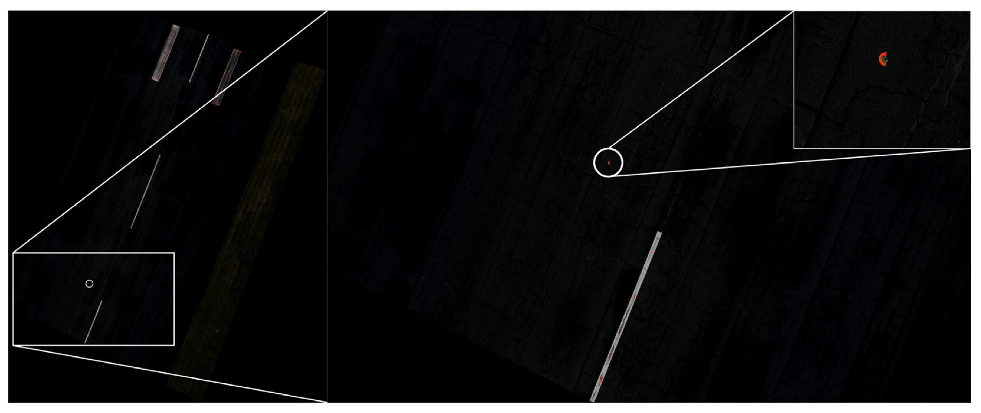
For the identification of field-vole holes and to compare methodologies, as they affected scattered areas, target areas were specified. The field-vole holes and the thermal images overlapping the target FOD were separately analyzed using FlirTools and DJI Thermal Analysis software [53].

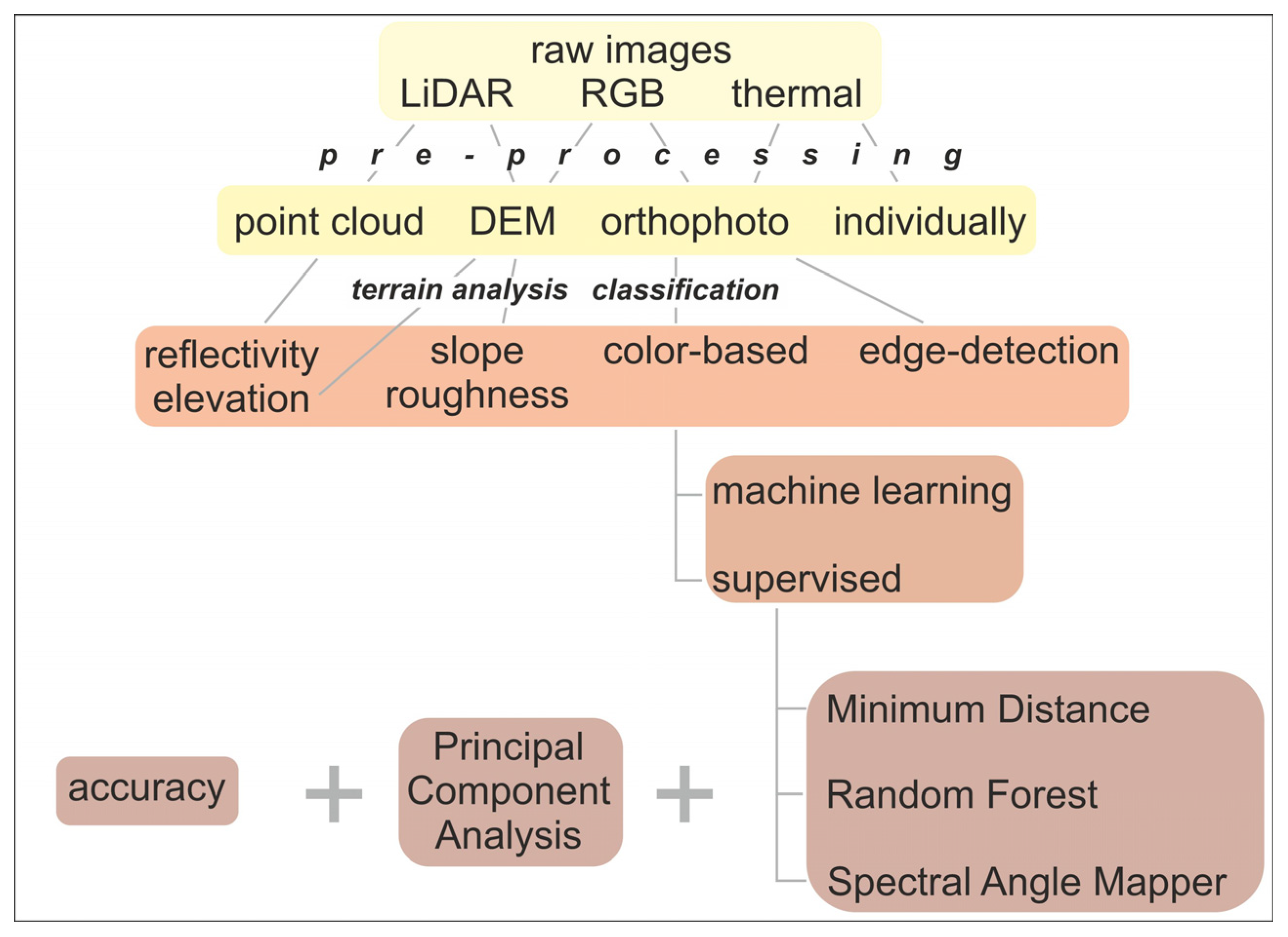
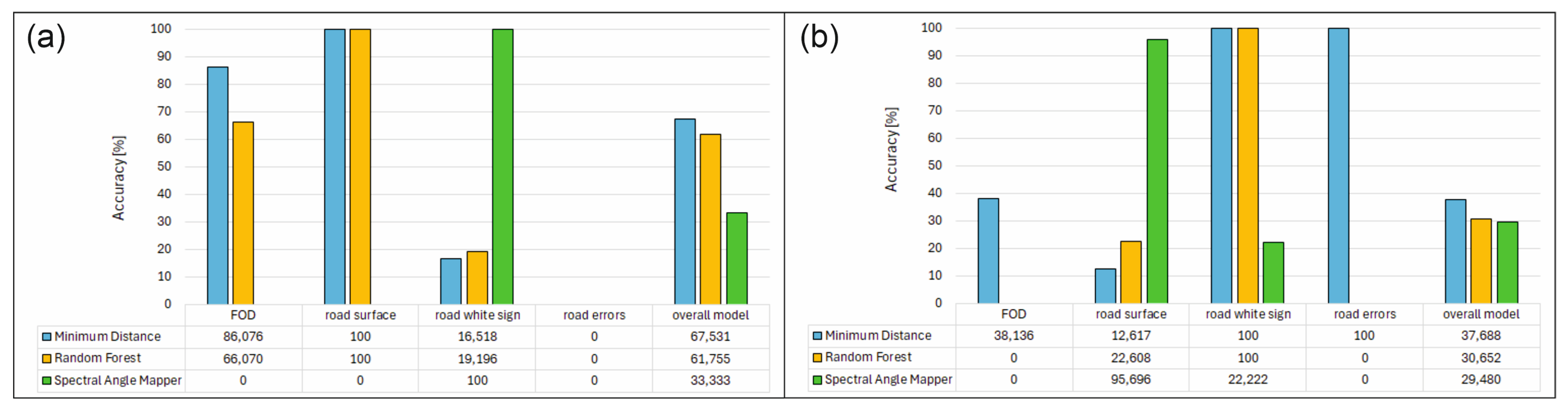
For the FOD test, different color searches were run on the orthomosaics, focusing primarily on the colors corresponding to the unique color composition of FOD A and FOD D. It was approached in two ways. In one case, a vector point layer was first created from the pixels of the bodies, then the band values of the overlapping raster pixels of both FOD were collected using the QGIS-‘Sample raster values’ algorithm. The procedure was performed based on both the RGB and LiDAR orthomosaics, and then the average, minimum, and maximum values characteristic of the bodies were determined for both cases. Based on the results of this color composition, a selection rule system was constructed and run on both orthomosaics using the Raster calculator.

In another case, the ROI polygons according to the bodies were trained using the QGIS SCP plugin [54], and the image classification was run with the Minimum Distance, Spectral Angle Mapping, and Random Forest algorithm. The Minimum Distance (MD) classification calculates the Euclidean distance d(x, y) between spectral signatures of image pixels and training spectral signatures, according to the following equation:

$$d\left(x,y\right)=\sqrt{{{\displaystyle \sum }}_{i=1}^n{\left(x_i-y_i\right)}^2}$$

(1)

where x is the first spectral signature vector, y is the second spectral signature vector, and n is the number of image bands. The SAM algorithms can be written as Equation (2):

$$\theta \left(x,y\right)=co{s}^{-1}\left(\frac{{{\displaystyle \sum }}_{i=1}^n{x}_i y_i}{{\left({{\displaystyle \sum }}_{i=1}^n{x}_i^2 \right)}^{\frac{1}{2}} \ast {\left({{\displaystyle \sum }}_{i=1}^n{y}_i^2\right)}^{\frac{1}{2}}}\right)$$

(2)

where x is the spectral signature vector of an image pixel, y is the spectral signature vector of a training area, and n shows the number of image bands. The Random Forest was based on decision trees and used the Gini index (Equation (3)) as the background of the calculations.

$$Gini index=1-{{\displaystyle \sum }}_{i=1}^n{\left(p_i\right)}^2$$

(3)

where $p_i$ is the fraction of items labeled with class i in the set. We created a confidence raster too where we can see the classification errors if pixels have low confidence values. After running the above classifications, the accuracy against the reference cover was assessed.

The created reference cover examined the results of PCA analysis, as in this case we were also working with a larger amount of data due to the spatial resolution. Principal Component Analysis (PCA) is a method for reducing the dimensions of measured variables (bands) to the principal components. The principal component transformation provides a new set of bands (principal components) having the following characteristic: principal components are uncorrelated and each component has a variance less than the previous component. The first principal components layers were first reclassified according to the classes used during training, and then used as the reference layer for accuracy assessment. The accuracy assessment is performed with the calculation of an error matrix. The error matrix can be evaluated from various perspectives. On one hand, it can gather data on how accurately a classification algorithm identifies the reference classes. On the other hand, it can examine how much the algorithm misclassifies. For FOD recognition, data were collected corresponding to the first perspective, and then graphically represented to assess which algorithm better facilitates FOD recognition.

Another way to find the FOD in the orthomosaic was edge detection. It is an image-processing technique that is used to identify the boundaries of objects. In a Python environment, OpenCV [55] was used with the following important steps: The first step is to convert the original image into grayscale. The next step is to apply thresholding to convert this grayscale image to a binary file. In this step, it is important to choose the threshold and maximum value and the thresholding type, which can be, e.g., binary, binary_inv, trunc, tozero, otsu, or triangle. The last step is to find the contours.

The processing chain is summarized in Figure 4.

3. Results

The road surface (Figure 5) exhibited a slight slope, which is conducive to water drainage considerations in planning. Each terrain analysis image revealed numerous minor road surface anomalies, which, however, did not result in discrepancies exceeding half a centimeter in the road surface. Both approaches complicate the search for FOD on the roadway.

3.1. FOD Recognition Results

The determination of the classification rules based on the terrain parameters (e.g., slope, roughness, elevation) is difficult to categorize in such a way that only the FOD are reliably included in the subsequent result from the point of view of accuracy. While the height analysis is hampered by the slope of the road surface that helps drainage, since although a specific FOD can be identified in a small area with height parameters, due to the slope, most of the road also corresponds to this height. Similarly, bump and slope analyses (combined with edge detection) make it difficult to distinguish between the many minor road defects. In the latter case, the appearance of closed shapes in the result images can help (see later).

3.1.1. LiDAR Results

The LIDAR-based terrain analysis results yielded the same experiences as the results run on the RGB DSM model. These will be presented in more detail with the RGB results. Here, we would like to highlight only the more important experiences related to LiDAR, and we would like to present the results related to the intensity values.

Classifying the LIDAR point cloud is also challenging due to the aforementioned difficulties. FOD points are often classified as road surfaces, further complicating the process. Identifying particularly thin, irregular, and non-closed objects (such as wires, cables, and FOD “C”) in a comprehensive terrain survey is nearly impractical, as it relies on precise “hits” and returns of signals from the sensor.

Sorting based on intensity and reflectivity values partially fulfilled the task (Figure 6). This approach will have to be further investigated, as the meteorological (primarily lighting) conditions were not the most optimal.

In the case of FOD “D”, it was not possible to significantly separate the body from road defects. In the case of the two larger foreign bodies, this LiDAR parameter could be used more effectively. But this may also depend on the material of the examined object. The two larger objects were metal (FOD “A”) and dark gray plastic (FOD “B”). While FOD “A” was separated nicely on the reflective image (Figure 6b), FOD “B”, despite its larger size, could hardly be separated. Even in terms of height parameters, it does not appear clearly, and in the end, its reflective properties did not make it clearly separable either. For the time being, it can be explained by the fact that, for some reason, this object may have absorbed the LiDAR signal during this measurement (due to the color itself, the composition of the plastic, and the surface moisture), and, on the other hand, the spectral properties of this dark plastic object may show minor differences from the asphalt pavement, like the other metallic body.

3.1.2. RGB Results

Using only the RGB camera, all of the FOD can be detected, no matter their size (Figure 7). Visual evaluation can be used in this case, but colorful FOD (“A” and “D”) can be found with algorithms too, even if they are very small. FOD “C” cannot be found with edge detection—if the roadway is maintained and faultless (without road faults), its irregular shape may be easier to detect, or if its color is not white or gray. The same color problem appears with FOD “B”: its color is very similar to the runway.

When creating a slope map, FOD “A” and “B” can be found and separated from other road roughness (Figure 8).

For FOD “D” and “A”, since these objects have a unique color, the result of the color-based classification can be seen in Figure 9 below.

As an inaccuracy of the method, we would like to point out here that in both cases, other road elements, mostly the more recent large-scale painting of the road, were also selected by the method (Arrow 1, Figure 9). The reason for this, however, can be attributed to poor lighting conditions rather than to the method.

From the point of view of surface diagnostics, we would highlight the road defects shown in Figure 9 as an advantage of the method. Cracks and repairs separate well. There is a difference between repaired (white cracks) and existing cracks (dark red) (Arrow 2, Figure 9). A crack pattern (dashed line) emerges, which may not be visible to the eye, yet since it runs uniformly along the entire road surface, it could indicate minor structural issues. All of these observations are also noticeable in the LiDAR intensity image (Figure 6b), where the wetter patches of the road surface are also a little bit more dominant.

In Figure 10, a detailed view of the results of supervised and machine-learning algorithms can be seen. The ones marked with 1 represent the results for FOD A, while those marked with 2 show the results for FOD D. Version (a) depicts the results of PCA, (b) shows the results of Minimum Distance (MD), (c) illustrates the confidence of MD, (d) shows the results of Random Forest (RF), and (e) characterizes the confidence of RF.

In contrast to the above, the Spectral Angle Mapper algorithm achieved weaker results, which can be attributed to the lack of reflectance values. FOD A was successfully detected by both MD and RF algorithms. However, from the results, we can also observe that road markings mostly cause errors in the automation process. Another crucial point is that besides FOD, the algorithms are also capable of reliably distinguishing road defects. In the case of Random Forest, it is worth noting that it separated repaired and existing road defects, although it classified unrepaired cracks as FOD (Figure 10(d1)).

The comparison of algorithm effectiveness is summarized in Figure 11.

For FOD detection, the Minimum Distance algorithm achieved the best results, performing the best when projected onto the entire model as well. Additionally, it exhibited fewer class swaps. This was followed by Random Forest classification. For RGB images, the application of these two algorithms is recommended. In addition to the classification algorithms, PCA also greatly supports data analysis. The development of automatic surface diagnostics will definitely benefit from the application of PCA analysis.

Edge detection was successful with FOD “A”; with the properly chosen parameters of the OpenCV algorithm, this FOD can be clearly separated and highlighted from the road, and only parts of the paintings appear (Figure 12). Since the size and shape of the other objects are the same as the road defects, their detection using this method is not possible unless the area to be examined is very small.

3.1.3. Thermal Results

The analysis of the road surface and FOD located on it was limited in this case due to constrained methodology. The primary reason for this was that the survey took place in cold conditions. Consequently, metallic and different material (plastic) objects did not “stand out” from the road surface under these circumstances. In cold weather, there was no difference in surface temperature. For these reasons, the orthorectification of the images of the road surface was impossible because too similar image data were generated, which could not be aligned in this manner. Therefore, the analysis of the road surface was conducted on individual images. However, in these images, traces of larger (rarely observed) cracks and mostly the FOD can be identified and analyzed (Figure 13). The orthorectification process could be performed in areas adjacent to the road.

In addition to examining the FOD, we would also like to point out in the thermal images in Figure 13 that cracks, road repairs (a), as well as moisture and drying out (b) can also be separated and examined.

3.2. Field-Vole Hole Recognition Results

The results of the LiDAR terrain analysis will not be detailed as they are similar to those of the RGB in this regard (Figure 14). The intensity data will be evaluated for this purpose in the near future, but can be partially seen in the top-left corner of Figure 6b.

3.2.1. RGB Results

For field-vole hole recognition, both the slope, TRI, and roughness layers produced as terrain analysis on the DSM model, as well as the height deviations, proved to be suitable. Among these, the results of the height analysis in Figure 14 can be observed. Their selection from other terrain variations is facilitated by density-based examination. Thus, the higher number of densely occurring, closed isolines indicates the presence of field-vole holes in the terrain (Figure 14).

3.2.2. Thermal Results

The thermal images in Figure 13 covered the same area as the orthophoto shown in Figure 14, and their vegetation cover was uniformly sparse. The thermal results also proved suitable for detecting field-vole holes. The mounds exhibited cooler thermal signatures under the current imaging conditions, as highlighted in Figure 15. This could primarily be attributed to the disturbed and bare ground being more moisture-laden under the prevailing meteorological conditions.

It is also noticeable that while the orthomosaics mainly show the mounds, holes, and occasionally the trails of grass trampling, the thermal images also reveal the extent of disturbed terrain. Since there were no differences in vegetation cover, the lower temperatures in certain areas could be explained by the extent of underground disturbance. This could be due to the cooler air and higher moisture content in the underground tunnels, resulting in larger-scale, significant temperature differences where a greater number of underground tunnels are present.

In Figure 15a,b, we also want to highlight that while most mounds appeared cooler, there were sporadic occurrences of “warmer mounds” (a) in the terrain. One possible explanation could be the timing, indicating fresher disturbances that heated up more compared to older mounds with higher moisture content. Another explanation could be the presence of living populations closer to the surface. Additionally, based on Figure 15, it is notable that while not every metallic terrain feature on the road surface was distinguishable in cold weather, every metallic feature on the ground surface significantly stood out (lower-right (a)/left (b) corner, channel grate).

4. Discussion

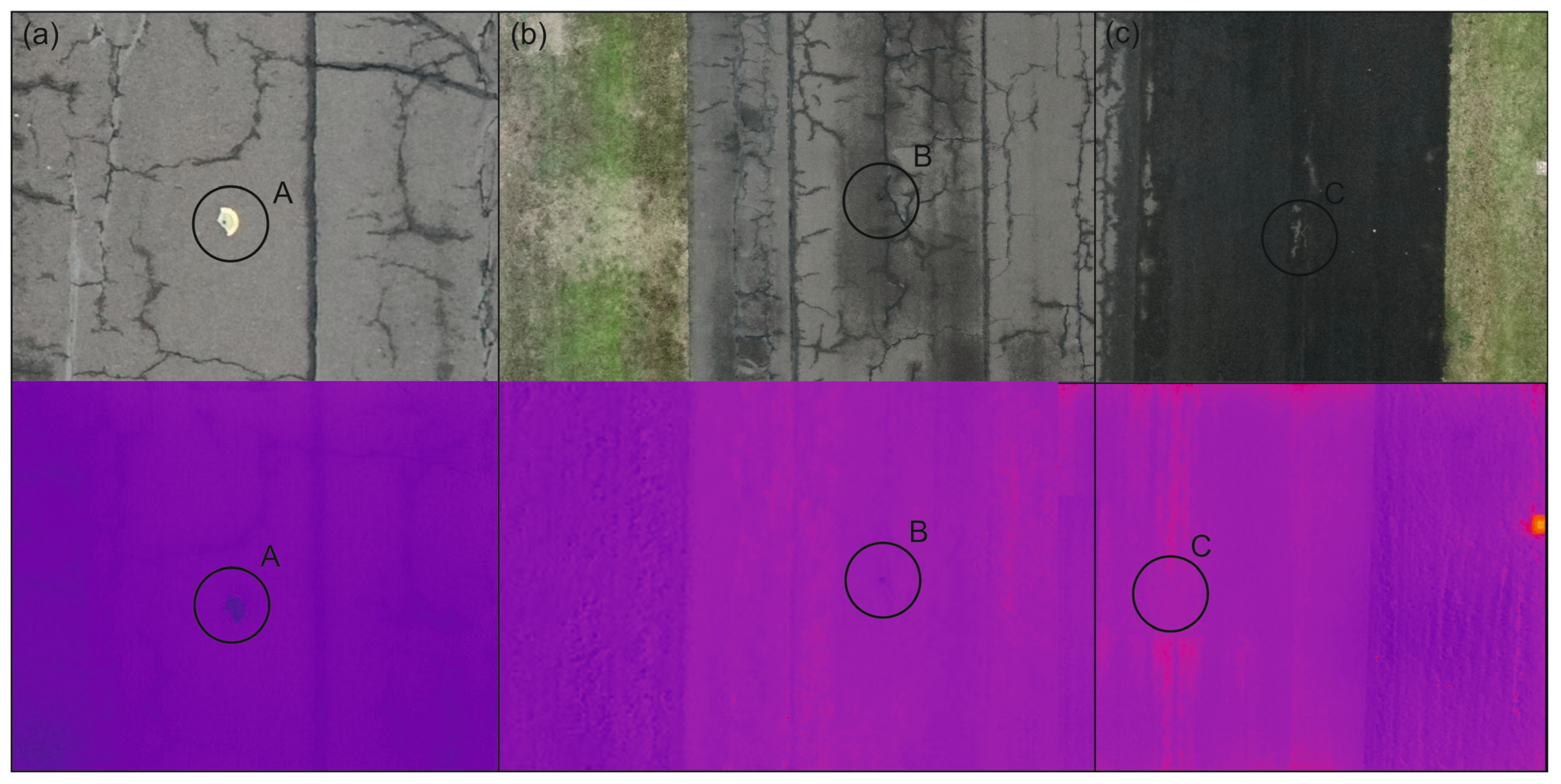
Our main research goal is to create and integrate a complex drone flight plan into an airport environment. The first step of this—which is the goal of this manuscript—is the examination of the recognition ability of different sensor systems, both in the field of FOD (Foreign Object Debris), surface diagnostics, and animal populations. In addition, data have been collected on the methodological effects of different meteorological and weather conditions.

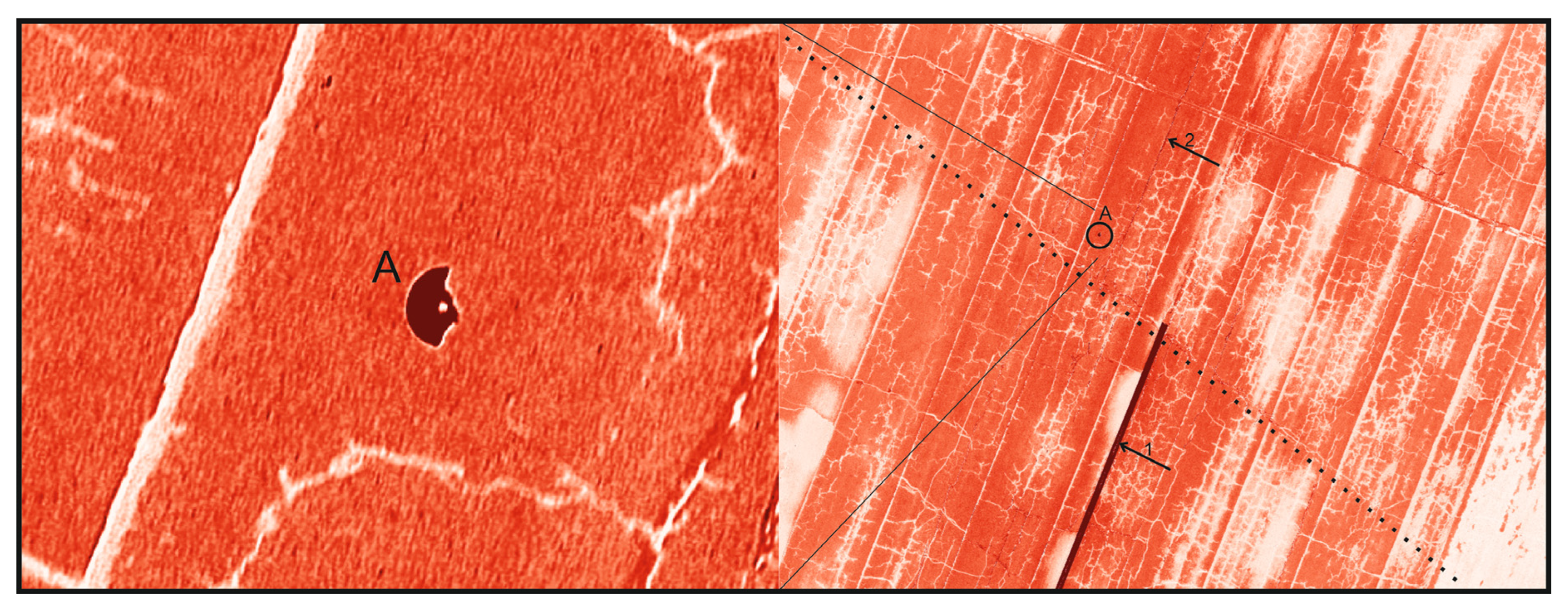
Although LiDAR analysis can achieve high accuracy and even small elevation differences can be measured, separating the different elements has proven difficult. Since most roads are designed to have some slope, methodological options to reduce the effect of slope should be further explored. For example, with mobile (car-mounted) LiDAR systems, an area of 20–30 m is scanned so that the base plane can be determined more easily, and classes that differ from it can be automatically searched with greater accuracy. Currently, although the LiDAR measurements, in addition to the nadir recording, were able to indicate the presence of stones, potholes, or microreflections, due to the difficulties in determining the base plane, the automatic methodology could not classify the surface deviations with sufficient accuracy. Overall, the analysis of LiDAR intensity values was found to be more beneficial compared to height values. The differences in the intensity values correlated with the road surface’s moisture content and repaired and unrepaired cracks. The examination of the absorption of plastic FOD objects by the LiDAR laser beam also requires further research. For this purpose, it will be advisable to check the recording using methods other than the nadir angle and to perform a LiDAR examination of different plastics.

According to the experience of the thermal sensors, the road surface in cold weather resulted in a too-uniform image, which is why the photogrammetric matching could not properly mosaic the area. This can be partially avoided at a higher flight height, but then the spatial resolution of the recordings deteriorates, which would make the examination of FOD impossible. Alternatively, the use of additional GCP points should be investigated. The result was primarily attributed to weather effects, as the unidentifiable FOD and the entire road surface became the same temperature. The thermal recording took place in the afternoon; however, there was not enough solar radiation, which could have been absorbed differently, so in winter and cold and cloudy weather, the thermal recordings may be associated with photogrammetric difficulties.

During the RGB image processing, no such difficulties have been experienced as in the case of previous sensors. The accuracy of the automatic sorting was challenged by a “color shift” (the image resolution is low for the size of the small object), so although all FOD were recognizable, during the automatic sorting, difficulties were experienced, mainly with road painting, but due to the different shape characteristics, the final conclusion could be drawn. The success of the FOD search with the presented sensors can be seen in

Table 3. The success of the FOD search with the presented sensors. Y = can be detected, N = cannot be detected, and N/A stands for no data available.

FOD/Sensor	L1 (Lidar)	P1 (RGB)	H20T (Thermal)
A (side light lamp subframe)	Y	Y	Y
B (tractor engine air filter)	N	Y	Y
C (wire)	N	Y	N
D (shotgun cartridge case)	N	Y	N/A

.

As part of the continuous data collection, it is necessary to carry out more precise reference checks, which we plan to supplement with the measurements of a multispectral camera in addition to the existing sensors. Currently, due to the difficulties of the thermal sensor—especially in cold weather conditions—it is challenging and time consuming to provide a reference for all surface deviations. Even though the LiDAR measurements indicated certain features such as rocks or microcracks, the additional image analysis could not fully help to confirm them. The success of the FOD search with the above-presented methods can be seen in

Table 4. The success of the FOD search with the presented methods. Y = can be detected, N = can not be detected.

FOD/Method	Terrain Analysis	Color-Based Classification	PCA	Supervised Classification	Edge Detection
A (side light lamp subframe)	Y	Y	Y	Y	Y
B (tractor engine air filter)	Y	N	Y	N	N
C (wire)	N	N	Y	N	N
D (shotgun cartridge case)	N	N	Y	Y	N

.

In the field of population analysis, the most versatile of the sensors and methods, besides RGB, are the results of the thermal sensor. In the future, it will be necessary to investigate how the measured data from the thermal sensor will be affected by the extent of vegetation. The thermal variations currently observed at the ground surface are currently attributed to subsurface tunnel but will need to be confirmed by field verification. The observability of these thermal differences under different vegetation cover and different weather conditions should be investigated.

5. Conclusions

As a pilot study, a basic survey was completed in the winter period, which can later serve as a reference for further measurements, and also helps to collect data on the expected effects of various weather conditions. Taking economic and usability aspects into account (preferably with fewer flights and sensors), it can be said that based on what has been carried out so far, the RGB camera is a suitable FOD regardless of size and other external factors (e.g., weather and light) and field-vole hole detection. Based on experience so far, it would be worthwhile to survey the area with a multispectral camera for better results.

From the perspective of airport applications (especially regarding military use), it is worth noting that the dominant DJI company in the drone market raises other questions as well. Therefore, it will be worthwhile to examine the compatibility of the respective sensors with other drone systems.

References

1. Rossi, G.; Tanteri, L.; Tofani, V.; Vannocci, P.; Moretti, S.; Casagli, N. Multitemporal UAV Surveys for Landslide Mapping and Characterization. Landslides 2018, 15, 1045–1052. [Google Scholar] [CrossRef]
2. Bonali, F.L.; Tibaldi, A.; Marchese, F.; Fallati, L.; Russo, E.; Corselli, C.; Savini, A. UAV-Based Surveying in Volcano-Tectonics: An Example from the Iceland Rift. J. Struct. Geol. 2019, 121, 46–64. [Google Scholar] [CrossRef]
3. Török, Á.; Bögöly, G.; Somogyi, Á.; Lovas, T. Application of UAV in Topographic Modelling and Structural Geological Mapping of Quarries and Their Surroundings—Delineation of Fault-Bordered Raw Material Reserves. Sensors 2020, 20, 489. [Google Scholar] [CrossRef] [PubMed]
4. Liu, X.; Zhu, W.; Lian, X.; Xu, X. Monitoring Mining Surface Subsidence with Multi-Temporal Three-Dimensional Unmanned Aerial Vehicle Point Cloud. Remote Sens. 2023, 15, 374. [Google Scholar] [CrossRef]
5. Yavuz, M.; Tufekcioglu, M. Assessment of Flood-Induced Geomorphic Changes in Sidere Creek of the Mountainous Basin Using Small UAV-Based Imagery. Sustainability 2023, 15, 11793. [Google Scholar] [CrossRef]
6. Hussain, Y.; Schlögel, R.; Innocenti, A.; Hamza, O.; Iannucci, R.; Martino, S.; Havenith, H.B. Review on the Geophysical and UAV-Based Methods Applied to Landslides. Remote Sens. 2022, 14, 4564. [Google Scholar] [CrossRef]
7. Tien Bui, D.; Long, N.Q.; Bui, X.-N.; Nguyen, V.-N.; Van Pham, C.; Van Le, C.; Ngo, P.-T.T.; Bui, D.T.; Kristoffersen, B. Lightweight Unmanned Aerial Vehicle and Structure-from-Motion Photogrammetry for Generating Digital Surface Model for Open-Pit Coal Mine Area and Its Accuracy Assessment. In Advances and Applications in Geospatial Technology and Earth Resources; Springer International Publishing: Cham, Switzerland, 2018; pp. 17–33. [Google Scholar]
8. Telli, K.; Kraa, O.; Himeur, Y.; Ouamane, A.; Boumehraz, M.; Atalla, S.; Mansoor, W. A Comprehensive Review of Recent Research Trends on UAVs. Systems 2023, 11, 400. [Google Scholar] [CrossRef]
9. Puri, V.; Nayyar, A.; Raja, L. Agriculture Drones: A Modern Breakthrough in Precision Agriculture. J. Stat. Manag. Syst. 2017, 20, 507–518. [Google Scholar] [CrossRef]
10. Primicerio, J.; Di Gennaro, S.F.; Fiorillo, E.; Genesio, L.; Lugato, E.; Matese, A.; Vaccari, F.P. A Flexible Unmanned Aerial Vehicle for Precision Agriculture. Precis. Agric. 2012, 13, 517–523. [Google Scholar] [CrossRef]
11. Zhang, C.; Kovacs, J.M. The Application of Small Unmanned Aerial Systems for Precision Agriculture: A Review. Precis. Agric. 2012, 13, 693–712. [Google Scholar] [CrossRef]
12. Mogili, U.R.; Deepak, B.B.V.L. Review on Application of Drone Systems in Precision Agriculture. Procedia Comput. Sci. 2018, 133, 502–509. [Google Scholar] [CrossRef]
13. Ahirwar, S.; Raghunandan Swarnkar, S.; Srinivas, B.; Namwade, G.; Swarnkar, R.; Bhukya, S. Application of Drone in Agriculture. Int. J. Curr. Microbiol. Appl. Sci. 2019, 8, 2500–2505. [Google Scholar] [CrossRef]
14. Lyons, M.B.; Brandis, K.J.; Murray, N.J.; Wilshire, J.H.; McCann, J.A.; Kingsford, R.T.; Callaghan, C.T. Monitoring Large and Complex Wildlife Aggregations with Drones. Methods Ecol. Evol. 2019, 10, 1024–1035. [Google Scholar] [CrossRef]
15. Corcoran, E.; Winsen, M.; Sudholz, A.; Hamilton, G. Automated Detection of Wildlife Using Drones: Synthesis, Opportunities and Constraints. Methods Ecol. Evol. 2021, 12, 1103–1114. [Google Scholar] [CrossRef]
16. Linchant, J.; Lisein, J.; Semeki, J.; Lejeune, P.; Vermeulen, C. Are Unmanned Aircraft Systems (UASs) the Future of Wildlife Monitoring? A Review of Accomplishments and Challenges. Mamm. Rev. 2015, 45, 239–252. [Google Scholar] [CrossRef]
17. Wang, D.; Shao, Q.; Yue, H. Surveying Wild Animals from Satellites, Manned Aircraft and Unmanned Aerial Systems (UASs): A Review. Remote Sens. 2019, 11, 1308. [Google Scholar] [CrossRef]
18. Cescutti, F.; Cefalo, R.; Coren, F. Application of Digital Photogrammetry from UAV Integrated by Terrestrial Laser Scanning to Disaster Management Brcko Flooding Case Study (Bosnia Herzegovina). In New Advanced GNSS and 3D Spatial Techniques; Lecture Notes in Geoinformation and Cartography; Springer: Cham, Switzerland, 2018; pp. 245–260. [Google Scholar]
19. Anderson, K.; Westoby, M.J.; James, M.R. Low-Budget Topographic Surveying Comes of Age: Structure from Motion Photogrammetry in Geography and the Geosciences. Prog. Phys. Geogr. 2019, 43, 163–173. [Google Scholar] [CrossRef]
20. Kyriou, A.; Nikolakopoulos, K.; Koukouvelas, I.; Lampropoulou, P. Repeated Uav Campaigns, Gnss Measurements, Gis, and Petrographic Analyses for Landslide Mapping and Monitoring. Minerals 2021, 11, 300. [Google Scholar] [CrossRef]
21. Gomez, C.; Purdie, H. UAV Based Photogrammetry and Geocomputing for Hazards and Disaster Risk Monitoring—A Review. Geoenviron. Disaster 2016, 3, 23. [Google Scholar] [CrossRef]
22. Naqvi, S.A.R.; Hassan, S.A.; Pervaiz, H.; Ni, Q. Drone-Aided Communication as a Key Enabler for 5G and Resilient Public Safety Networks. IEEE Commun. Mag. 2018, 56, 36–42. [Google Scholar] [CrossRef]
23. Greenwood, W.W.; Lynch, J.P.; Zekkos, D. Applications of UAVs in Civil Infrastructure. J. Infrastruct. Syst. 2019, 25, 04019002. [Google Scholar] [CrossRef]
24. Shakhatreh, H.; Sawalmeh, A.H.; Al-Fuqaha, A.; Dou, Z.; Almaita, E.; Khalil, I.; Othman, N.S.; Khreishah, A.; Guizani, M. Unmanned Aerial Vehicles (UAVs): A Survey on Civil Applications and Key Research Challenges. IEEE Access 2019, 7, 48572–48634. [Google Scholar] [CrossRef]
25. Manfreda, S.; McCabe, M.F.; Miller, P.E.; Lucas, R.; Pajuelo Madrigal, V.; Mallinis, G.; Ben Dor, E.; Helman, D.; Estes, L.; Ciraolo, G.; et al. On the Use of Unmanned Aerial Systems for Environmental Monitoring. Remote Sens. 2018, 10, 641. [Google Scholar] [CrossRef]
26. Yoo, L.S.; Lee, J.H.; Lee, Y.K.; Jung, S.K.; Choi, Y. Application of a Drone Magnetometer System to Military Mine Detection in the Demilitarized Zone. Sensors 2021, 21, 3175. [Google Scholar] [CrossRef] [PubMed]
27. Ko, Y.; Kim, J.; Duguma, D.G.; Astillo, P.V.; You, I.; Pau, G. Drone Secure Communication Protocol for Future Sensitive Applications in Military Zone. Sensors 2021, 21, 2057. [Google Scholar] [CrossRef] [PubMed]
28. Edelman, H.; Stenroos, J.; Queralta, J.P.; Hästbacka, D.; Oksanen, J.; Westerlund, T.; Röning, J. Analysis of Airport Design for Introducing Infrastructure for Autonomous Drones Infrastructure for Autonomous Drones. Emerald Insight 2023, 41, 263–2772. [Google Scholar] [CrossRef]
29. Martinez, C.; Sanchez-Cuevas, P.J.; Gerasimou, S.; Bera, A.; Olivares-Mendez, M.A. Sora Methodology for Multi-Uas Airframe Inspections in an Airport. Drones 2021, 5, 141. [Google Scholar] [CrossRef]
30. LHSN SZOLNOK—Minden Dokumentum. Available online: https://www.ket.hm.gov.hu/milaiphun/Megosztott%20dokumentumok/Forms/AllItems.aspx?RootFolder=%2Fmilaiphun%2FMegosztott%20dokumentumok%2FMILAIP%2FPart%203%20AERODROMES%20%28AD%29%2FAERODROMES%202%2FLHSN%20SZOLNOK&FolderCTID=0x01200005F7E2F6A0763B489FB0273C8D5D9532&View=%7B3CC9DF8E%2DBB97%2D4202%2D8765%2D273B2108092C%7D (accessed on 29 February 2024).
31. 26/2007. (III. 1.) GKM-HM-KvVM Együttes Rendelet a Magyar Légtér Légiközlekedés Céljára Történő Kijelöléséről—Hatályos Jogszabályok Gyűjteménye. Available online: https://net.jogtar.hu/jogszabaly?docid=a0700026.gkm (accessed on 29 February 2024).
32. Implementing Regulation—2019/947—EN—EUR-Lex. Available online: https://eur-lex.europa.eu/eli/reg_impl/2019/947/oj (accessed on 29 February 2024).
33. Regulation—2018/1139—EN—EUR-Lex. Available online: https://eur-lex.europa.eu/eli/reg/2018/1139/oj (accessed on 29 February 2024).
34. 4/1998. (I. 16.) Korm. Rendelet a Magyar Légtér Igénybevételéről—Hatályos Jogszabályok Gyűjteménye. Available online: https://net.jogtar.hu/jogszabaly?docid=99800004.kor (accessed on 29 February 2024).
35. Salour, F. Moisture Influence on Structural Behaviour of Pavements; Field and Laboratory Investigations, KTH, Royal Institute of Technology School of Architecture and the Built Environment: Stockholm, Sweden, 2015. [Google Scholar]
36. Naotunna, C.N.; Samarakoon, S.M.S.M.K.; Fosså, K.T. Experimental Investigation of Crack Width Variation along the Concrete Cover Depth in Reinforced Concrete Specimens with Ribbed Bars and Smooth Bars. Case Stud. Constr. Mater. 2021, 15, e00593. [Google Scholar] [CrossRef]
37. Rokitowski, P.; Bzówka, J.; Grygierek, M. Influence of High Moisture Content on Road Pavement Structure: A Polish Case Study. Case Stud. Constr. Mater. 2021, 15, e00594. [Google Scholar] [CrossRef]
38. Elseicy, A.; Alonso-Díaz, A.; Solla, M.; Rasol, M.; Santos-Assunçao, S. Combined Use of GPR and Other NDTs for Road Pavement Assessment: An Overview. Remote Sens. 2022, 14, 4336. [Google Scholar] [CrossRef]
39. Foreign Object Debris (FOD)|SKYbrary Aviation Safety. Available online: https://skybrary.aero/articles/foreign-object-debris-fod (accessed on 29 February 2024).
40. A Légierő Napját Ünnepelték Szolnokon. Available online: https://airportal.hu/a-legiero-napjat-unnepeltek-szolnokon/ (accessed on 29 February 2024).
41. Arrival of New H225M Helicopters Is a Milestone in Armed Forces Development. Available online: https://defence.hu/news/arrival-of-new-h225m-helicopters-is-a-milestone-in-armed-forces-development.html (accessed on 29 February 2024).
42. MH 86. Szolnok Helikopter Bázis—Családi Nap, 2022. Május 28—YouTube. Available online: https://www.youtube.com/watch?v=UFBNkV_pnAc (accessed on 29 February 2024).
43. Matrice 350 RTK—DJI. Available online: https://enterprise.dji.com/matrice-350-rtk (accessed on 29 February 2024).
44. Zenmuse L1—UAV Load Gimbal Camera—DJI Enterprise. Available online: https://enterprise.dji.com/zenmuse-l1 (accessed on 29 February 2024).
45. Zenmuse H20 Series—UAV Load Gimbal Camera—DJI Enterprise. Available online: https://enterprise.dji.com/zenmuse-h20-series (accessed on 29 February 2024).
46. Zenmuse P1—UAV Load Gimbal Camera—DJI Enterprise. Available online: https://enterprise.dji.com/zenmuse-p1 (accessed on 29 February 2024).
47. Drón Törvény 2021—Érthetően Szakértőktől—Légtér.Hu Kft. Available online: https://legter.hu/blog/dron-torveny-2021-erthetoen-szakertoktol/ (accessed on 18 September 2023).
48. A Drónozás Szabályai. Available online: https://www.djiars.hu/blogs/news/a-dronozas-szabalyai (accessed on 18 September 2023).
49. DJI Terra—Make the World Your Digital Asset—DJI. Available online: https://enterprise.dji.com/dji-terra (accessed on 19 May 2024).
50. LAStools: Converting, Filtering, Viewing, Processing, and Compressing LIDAR Data in LAS and LAZ Format. Available online: https://lastools.github.io/ (accessed on 19 May 2024).
51. GDAL Tools Plugin. Available online: https://docs.qgis.org/2.18/en/docs/user_manual/plugins/plugins_gdaltools.html (accessed on 19 May 2024).
52. ExifTool by Phil Harvey. Available online: https://exiftool.org/ (accessed on 19 May 2024).
53. DJI Thermal Analysis Tool 3—Download Center—DJI. Available online: https://www.dji.com/hu/downloads/softwares/dji-dtat3 (accessed on 19 May 2024).
54. Congedo, L. Semi-Automatic Classification Plugin: A Python Tool for the Download and Processing of Remote Sensing Images in QGIS. J. Open Source Softw. 2021, 6, 3172. [Google Scholar] [CrossRef]
55. OpenCV—Open Computer Vision Library. Available online: https://opencv.org/ (accessed on 19 May 2024).
Figure 1. Study area of Szolnok Hungarian Air Base.
Drones 08 00231 g001
Figure 2. Used equipment: (a) DJI Matrice 350 UAV, (b) controller, and (c) the RTK base station.
Drones 08 00231 g002
Figure 3. The two objectives of the study: (a) FOD detection and (b1,b2) field-vole (Mus spicilegus) holes.
Drones 08 00231 g003
Figure 4. The used tools of the processing chain.
Drones 08 00231 g004
Figure 5. The study area is shown in DTM and orthophoto with the examined FOD and field-vole holes. The DTM was made from the lidar point cloud, and the orthophoto was created based on the same (lower-resolution) lidar-connected RGB camera.
Drones 08 00231 g005
Figure 6. FOD “A” can be recognizable in the (a) RGB point cloud and in the (b) reflectance map.
Drones 08 00231 g006
Figure 7. FOD (A, B, C, D) in the RGB orthophoto (ad). All of them are recognizable by visual evaluation.
Drones 08 00231 g007
Figure 8. FOD (a) “A” and (b) “B” in the slope map. Other roughness (e.g., pavement) can be detected too, but the closed, elliptical shape is obvious. In (b), the lamp on the grass can be identified too.
Drones 08 00231 g008
Figure 9. FOD “A” after the color-based classification. The white road painting (1) has the same red color, but its shape and size are obviously different from the FOD. (2) Corrected road faults. Larger (contiguous) faults along the dashed line may indicate downslope movements.
Drones 08 00231 g009
Figure 10. Results of supervised and machine learning algorithms. Images with 1 represent the results for FOD A, while images with 2 show the results for FOD D. Version (a) depicts the results of PCA, (b) shows the results of Minimum Distance (MD), (c) illustrates the confidence of MD, (d) shows the results of Random Forest (RF), and (e) characterizes the confidence of RF.
Drones 08 00231 g010
Figure 11. The accuracy % of the algorithm at the class level as well as projected onto the entire model: (a) shows the results of the FOD A area, and (b) the FOD D area.
Drones 08 00231 g011
Figure 12. FOD “A” can be clearly detected with edge detection.
Drones 08 00231 g012
Figure 13. Thermal images of (a) FOD “A”, (b) FOD “B”, and (c) FOD “C”. The specific temperature value was not important, only the detection of the FOD (its separation from the ambient temperature in a positive or negative direction).
Drones 08 00231 g013
Figure 14. Field-vole holes in (a) the RGB orthophoto and (b) the DTM with 1 cm contour lines. Smaller, roughly circular lines may represent the holes (red arrows).
Drones 08 00231 g014
Figure 15. Field-vole holes in the thermal pictures. In (a,b), colder areas can be detected as holes. In (a), a warmer point can be seen too—possibly in this hole there is a living animal. See details in text.
Drones 08 00231 g015