Distributed Finite-Time ESO-Based Consensus Control for Multiple Fixed-Wing UAVs Subjected to External Disturbances

Abstract

This paper puts forward a coordinated formation control scheme for multiple fixed-wing unmanned aerial vehicle (UAV) systems with external nonlinear disturbances including not only the drag force and uncertain lateral force, but also the drag, lift, and lateral forces caused by wake vortices. A novel distributed finite-time extended state observer is designed to estimate both the unmeasurable states and uncertain external nonlinear disturbances of each fixed-wing UAV. In particular, an event-triggered mechanism is employed to reduce the burden of communication networks among multiple fixed-wing UAVs. Meanwhile, an inter-trigger output predictor, replacing the classic zero-order holder, is adopted to obtain cooperative errors between two consecutive triggering moments. Furthermore, a composite distributed controller is proposed to mitigate uncertain disturbances, enabling the coordinated formation flying of multiple fixed-wing UAVs.Finally, two illustrative simulation scenarios are discussed to verify the performance of the presented coordinated formation control scheme.

1. Introduction

Currently, fixed-wing unmanned aerial vehicles (UAVs) have many potential applications, such as resource exploration, border patrol, environmental monitoring, agricultural production, relief and rescue, and logistics transportation [1,2,3,4]. However, a single fixed-wing UAV las limited endurance and carrying capacity, which greatly limits its application in complex tasks. Consequently, extensive research efforts have been dedicated to studying both collaborative control and formation flying of multiple UAVs [5]. Due to the reliability, flexibility, and multi-task execution capabilities of UAVs’ in collaborative control and formation, flight efficiency, safety, and mission accomplishment can be significantly improved. So far, a variety of formation control schemes for multiple unmanned systems have been proposed, such as the leader–follower structure [6,7], consensus-based cooperative control [8,9,10,11], and virtual structure [12]. However, as a typical multi-variable complex underactuated system, the dynamics of fixed-wing UAVs contain strong coupling and uncertain external disturbances, resulting in a serious challenge in the design of formation control schemes. Meanwhile, the burden on communication channel bandwidth escalates rapidly with the increase in members within the UAV swarm, resulting in delays or losses in information transmission [13,14].

Estimating and rejecting disturbances or uncertainties for formation flying control of multiple UAVs has garnered considerable interest. For instance, disturbance observer-based control [15,16], sliding mode control [17,18], adaptive control [19], and intelligent control [20], as well as the references therein, have been explored. An adaptive leader–follower formation control strategy has been exploited to address unknown disturbances, including model uncertainties and external wind disturbances [17]. A disturbance observer-based formation-containment controller has been investigated to eliminate the negative effects of external disturbances in UAVs systems [13]. Further, as an anti-disturbance strategy independent of the system model, active disturbance rejection control (ADRC) using an extended state observer (ESO) has been widely studied for nonlinear systems with uncertainties/disturbances [21,22,23]. To achieve a superior performance for a fixed-wing UAVs, a robust control approach employing an ESO has been designed to deal with internal and external uncertainties [24].

The information exchange within multiple fixed-wing UAV formation systems is carried out via wireless communication networks. The inherent bandwidth limitations of communication networks result in adverse network phenomena during information transmission between adjacent UAVs, for instance packet dropouts and communication delays. As a consequence, different event-triggered mechanisms (ETMs) have been studied and put forward to reduce communication burden among members in a fixed-wing UAV swarm [13,25]. In [26], a static ETM has been designed to reduce the data transmission rates of control signals and to save on communication network resources in six-degree-of-freedom UAVs. A dynamic ETM has been devised to avoid unnecessary information exchanges among multiple fixed-wing UAVs [27]. A distributed adaptive ETM has been implemented to enhance the efficiency of data transmission for each fixed-wing UAV [13]. In particular, the design of formation of flying controllers for continuous-time systems containing an ETM, Zeno behavior must be considered in order to guarantee a positive lower bound between two consecutive triggering moments [25,28,29]. In addition, zero-order holders (ZOHs) are often employed to maintain the information between two adjacent triggering moments [25,30]. Significantly, although the event-triggered control reduces the burden of communication networks, the control accuracy of the studied system is inevitably not compromised, which implies that ETM cannot easily be applied to hard real-time systems such as high maneuverable fixed-wing UAVs [27].

Compared with disturbances and uncertainties rejection methods in the existing literature, the ADRC method possesses two remarkable advantages for achieving the formation flying of a UAV swarm: (1) it is independent of the dynamic model, which simplifies the modeling process, and (2) the estimation of relative velocity information and external disturbances relies solely on the relative position information, reducing the requirements for measuring equipment and communication burden. On the other hand, existing ETMs reduce the communication burden at the expense of accuracy loss. It is quite difficult to balance the contradiction between the limited relative information transmitted by ETMs and the collaborative control accuracy. In this paper, we aim to propose an ETM-based ADRC method to formulate the distributed collaboration control strategy for a fixed-wing UAV swarm. In particular, this paper’s contributions are as follows: (1) A novel distributed finite-time ESO is put forward for each fixed-wing UAV to estimate its uncertain disturbances and unmeasured states, only using the position information of the neighbors; (2) to predict the consensus error of the neighboring fixed-wing UAVs between two consecutive event-triggering instants, an inter-trigger output predictor is designed; (3) to realize the consensus control of a fixed-wing UAV swarm, a composite distributed controller is presented in terms of the distributed finite-time ESO.

The remainder of this paper is organized as follows. The dynamic model of fixed-wing UAVs is formulated in Section 2. Section 3 discusses a distributed finite-time ESO-based control strategy. In order to verify its performance, two illustrative numerical examples are displayed in Section 4. Conclusions are provided in Section 5.

2. Problem Formulation

The motion of the ith fixed-wing UAV can be formulated as [31]

$$\begin{array}{ccc}& & {\dot{x}}_i={\upsilon }_{i}cos\left({\gamma }_i\right)cos\left({\chi }_i\right),\hfill \\ & & {\dot{y}}_i={\upsilon }_{i}cos\left({\gamma }_i\right)sin{\chi }_i,\hfill \\ & & {\dot{z}}_i=-{\upsilon }_{i}sin{\gamma }_i,\hfill \\ & & {\dot{\upsilon }}_i=\frac{T_i}{m_i}-gsin{\gamma }_i+d_{\upsilon i},\hfill \\ & & {\dot{\gamma }}_i=\frac{g}{{\upsilon }_i}\left(n_{i}cos{\varphi }_i-cos{\gamma }_i\right)+d_{\gamma i},\hfill \\ & & {\dot{\chi }}_i=\frac{g}{{\upsilon }_i}\left(\frac{n_{i}sin{\varphi }_i}{cos{\gamma }_i}\right)+d_{\chi i},\hfill \end{array}$$

(1)

where $x_i$, $y_i$, and $z_i$ indicate the inertial position components of the ith UAV; ${\upsilon }_i$, ${\gamma }_i$, and ${\chi }_i$ represent the ground speed, flight-path angle, and heading angle, respectively. $m_i$ and g are the mass and gravity acceleration, respectively, and $T_i$, $n_i$, and ${\varphi }_i$ denote the control inputs, i.e., engine thrust, load factor, and banking angle, respectively. Thereafter, the throttle and elevator are employed to adjust the engine thrust and load factor, while the rudder and ailerons are adopted to control the banking angle. The external disturbances of $d_{\upsilon i}$, $d_{\gamma i}$, and $d_{\chi i}$ are expressed as

$$\begin{array}{ccc}& & d_{\upsilon i}=-\frac{D_i+\Delta D_i}{m_i},d_{\gamma i}=-\frac{\Delta L_{i}cos{\varphi }_i-(Y_i+\Delta Y_i)sin{\varphi }_i}{m_i{\upsilon }_i},\hfill \\ & & d_{\chi i}=-\frac{\Delta L_{i}sin{\varphi }_i-(Y_i+\Delta Y_i)cos{\varphi }_i}{m_i{\upsilon }_{i}cos{\gamma }_i},\hfill \end{array}$$

and $D_i$, $Y_i$ represent the drag force and uncertain lateral force, respectively; the drag deviation $\Delta D_i$, lift deviation $\Delta L_i$, and lateral deviation $\Delta Y_i$ are caused by wake vortices.

By introducing three virtual control inputs of $u_{xi}$, $u_{yi}$ and $u_{zi}$, system (1) can be rewritten as

$$\begin{array}{ccc}& & {\ddot{x}}_i=u_{xi}+d_{xi},\hfill \\ & & {\ddot{y}}_i=u_{yi}+d_{yi},\hfill \\ & & {\ddot{z}}_i=u_{zi}+d_{zi},\hfill \end{array}$$

(2)

where the relationship between the virtual control inputs of $u_{xi}$, $u_{yi}$, $u_{zi}$ and actual control inputs of $T_i$, $n_i$, ${\varphi }_i$ are given as

$$\begin{array}{ccc}& & T_i=[(g-u_{zi})sin{\gamma }_i+(u_{xi}cos{\chi }_i+u_{yi}sin{\chi }_i)cos{\gamma }_i]m_i,\hfill \\ & & n_i=\frac{(g-u_{zi})cos{\gamma }_i-(u_{xi}cos{\chi }_i+u_{yi}sin{\chi }_i)sin{\gamma }_i}{gcos{\varphi }_i},\hfill \\ & & {\varphi }_i=arctan\frac{u_{yi}cos{\chi }_i-u_{xi}sin{\chi }_i}{(g-u_{zi})cos{\gamma }_i-(u_{xi}cos{\chi }_i+u_{yi}sin{\chi }_i)sin{\gamma }_i},\hfill \end{array}$$

and the uncertain disturbances $d_{xi}$, $d_{yi}$, and $d_{zi}$ are

$$\begin{array}{ccc}& & d_{xi}=d_{\upsilon i}cos{\gamma }_{i}cos{\chi }_i-d_{\gamma i}{\upsilon }_{i}sin{\gamma }_{i}cos{\chi }_i-d_{\chi i}{\upsilon }_{i}cos{\gamma }_{i}sin{\chi }_i,\hfill \\ & & d_{yi}=d_{\upsilon i}cos{\gamma }_{i}sin{\chi }_i-d_{\gamma i}{\upsilon }_{i}sin{\gamma }_{i}sin{\chi }_i+d_{\chi i}{\upsilon }_{i}cos{\gamma }_{i}cos{\chi }_i,\hfill \\ & & d_{zi}=-d_{\upsilon i}sin{\gamma }_i-d_{\gamma i}{\upsilon }_{i}cos{\gamma }_i.\hfill \end{array}$$

Set $X_{i1}\left(t\right)={[x_i,y_i,z_i]}^T$, $X_{i2}\left(t\right)={[{\dot{x}}_i,{\dot{y}}_i,{\dot{z}}_i]}^T$, $U_i={[u_{xi},u_{yi},u_{zi}]}^T$ and $d_i\left(t\right)={[d_{xi},d_{yi},d_{zi}]}^T$. A compact form of (2) can be further obtained as

$$\begin{array}{ccc}& & {\dot{X}}_{i1}\left(t\right)=X_{i2}\left(t\right),\hfill \\ & & {\dot{X}}_{i2}\left(t\right)=U_i\left(t\right)+d_i\left(t\right),\hfill \\ & & M_i\left(t\right)=X_{i1}\left(t\right),\hfill \end{array}$$

(3)

where $M_i\left(t\right)$ represents the measurement output; $d_i\left(t\right)$ denotes the total disturbances.

The virtual leader’s dynamic model is

$$\begin{array}{ccc}& & {\dot{X}}_{01}\left(t\right)=X_{02}\left(t\right),\hfill \\ & & {\dot{X}}_{02}\left(t\right)=U_0\left(t\right),\hfill \\ & & M_0\left(t\right)=X_{01}\left(t\right).\hfill \end{array}$$

(4)

Set the consensus errors ${\tilde{X}}_{i1}\left(t\right)=X_{i1}\left(t\right)-X_{01}\left(t\right)$ and ${\tilde{X}}_{i2}\left(t\right)=X_{i2}\left(t\right)-X_{02}\left(t\right)$. From (3) and (4), the consensus error system describing the ith UAV relative to the virtual leader is

$$\begin{array}{ccc}& & {\dot{\tilde{X}}}_{i1}\left(t\right)={\dot{\tilde{X}}}_{i2}\left(t\right),\hfill \\ & & {\dot{\tilde{X}}}_{i2}\left(t\right)=U_i\left(t\right)+d_i\left(t\right)-U_0\left(t\right).\hfill \end{array}$$

(5)

Assumption 1

([21,22,23]). The control input $U_0\left(t\right)$ and total disturbances $d_i\left(t\right)$ are assumed to be continuously differentiable relative to time t, respectively. Moreover, a positive constant $h_i$ satisfies

$$\begin{array}{c}\hfill \parallel {\dot{d}}_i\left(t\right)\parallel +\parallel {\dot{U}}_0\left(t\right)\parallel \le h_i.\end{array}$$

In this paper, a directed graph $\mathcal{G}=\left\{\mathcal{V},ϵ,\mathcal{A}\right\}$ is employed to depict the position information exchange among a fixed-wing UAV swarm, where $\mathcal{V}=\left\{1,2,\dots ,n\right\}$, and $ϵ\in \mathcal{V}\times \mathcal{V}$ indicate the set of nodes and edges, respectively. Edge $(j,i)\in ϵ$ represents ith fixed-wing UAV, which can be used to obtain the position information from jth fixed-wing UAV. $a_{ij}$ in the nonnegative adjacency matrix $\mathcal{A}={\left[a_{ij}\right]}_{n\times n}$, which can be defined as

$$\begin{array}{c}\hfill a_{ij}=\left\{\begin{array}{c}0,if(j,i)\notin ϵ,\\ 1,if(j,i)\in ϵ.\end{array}\right.\end{array}$$

This paper aims to deal with the consistent collaborative or formation flying control in terms of the virtual leader for a fixed-wing UAV swarm with uncertain disturbances. More specifically, a control strategy for each member UAV is designed, such that the consensus errors $\underset{t\to \infty }{lim}\parallel {\tilde{X}}_{i1}\left(t\right)\parallel =0$ and $\underset{t\to \infty }{lim}\parallel {\tilde{X}}_{i2}\left(t\right)\parallel =0$ or $\underset{t\to \infty }{lim}\parallel X_{i1}\left(t\right)\parallel =X_{id}^1\left(t\right)$, $\underset{t\to \infty }{lim}\parallel X_{i2}\left(t\right)\parallel =X_{id}^2\left(t\right)$, where $X_{id}^1\left(t\right)$ and $X_{id}^2\left(t\right)$ represent the desired states of the ith UAV in the formation configuration.

3. Main Results

This section aims to put forward an ETM-based ADRC for the consensus control of multiple fixed-wing UAVs. Figure 1 shows the control scheme, consisting of an event-trigger, an inter-trigger output predictor, a distributed finite-time ESO, and a distributed anti-disturbance controller.

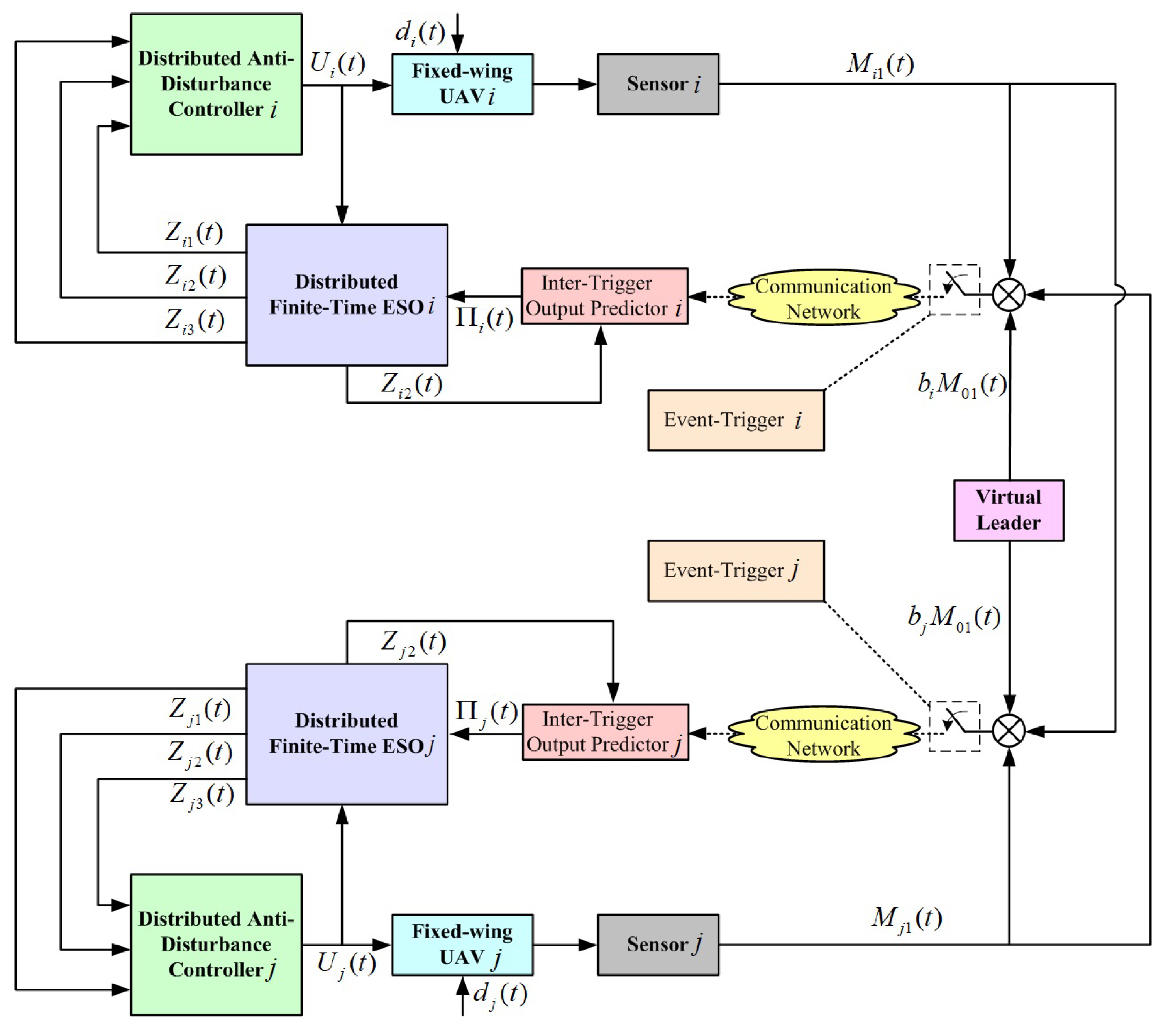
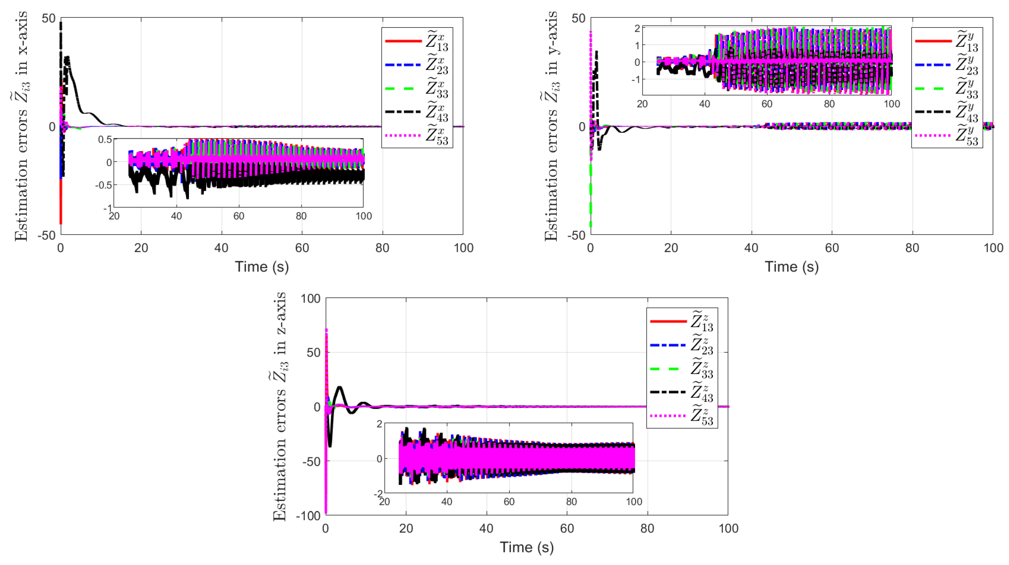
3.1. Distributed Finite-Time ESO

To simultaneously estimate the unmeasurable states and total disturbances, a distributed finite-time ESO is put forward in this subsection for each fixed-wing UAV. By setting ${\tilde{X}}_{i3}\left(t\right)=d_i\left(t\right)-U_0\left(t\right)$ and ${\dot{\tilde{X}}}_{i3}\left(t\right)=H_i\left(t\right)$, the consensus error system (5) is extended as

$$\begin{array}{ccc}& & {\dot{\tilde{X}}}_{i1}\left(t\right)={\tilde{X}}_{i2}\left(t\right),\hfill \\ & & {\dot{\tilde{X}}}_{i2}\left(t\right)=U_i\left(t\right)+{\tilde{X}}_{i3}\left(t\right),\hfill \\ & & {\dot{\tilde{X}}}_{i3}\left(t\right)=H_i\left(t\right).\hfill \end{array}$$

(6)

For the extended systems (6), the distributed finite-time ESO is constructed as

$$\begin{array}{cc}\hfill & {\dot{Z}}_{i1}\left(t\right)=-{\beta }_{i1}{G}_{i1}\left(Z_{i1}\left(t\right)-{\Pi }_i\left(t\right)\right)+Z_{i2}\left(t\right),\hfill \end{array}$$

(7a)

$$\begin{array}{cc}\hfill & {\dot{Z}}_{i2}\left(t\right)=-{\beta }_{i2}{G}_{i2}\left(Z_{i1}\left(t\right)-{\Pi }_i\left(t\right)\right)+Z_{i3}\left(t\right)+U_i\left(t\right),\hfill \end{array}$$

(7b)

$$\begin{array}{cc}\hfill & {\dot{Z}}_{i3}\left(t\right)=-{\beta }_{i3}{G}_{i3}\left(Z_{i1}\left(t\right)-{\Pi }_i\left(t\right)\right),\hfill \end{array}$$

(7c)

in which $Z_{i1}\left(t\right)$, $Z_{i2}\left(t\right)$ and $Z_{i3}\left(t\right)$ denote the estimation states of ${\tilde{X}}_{i1}\left(t\right)$, ${\tilde{X}}_{i2}\left(t\right)$ and ${\tilde{X}}_{i3}\left(t\right)$; ${\beta }_{i1}$, ${\beta }_{i2}$ and ${\beta }_{i3}$ are adjustable gain parameters; $G_{i1}\left(Z_{i1}\left(t\right)-{\Pi }_i\left(t\right)\right)$, $G_{i2}\left(Z_{i1}\left(t\right)-{\Pi }_i\left(t\right)\right)$, and $G_{i3}\left(Z_{i1}\left(t\right)-{\Pi }_i\left(t\right)\right)$ stand for nonlinear functions, depending on the estimation error $Z_{i1}\left(t\right)-{\Pi }_i\left(t\right)$, which are provided as

$$\begin{array}{ccc}& & G_{i1}\left(Z_{i1}\left(t\right)-{\Pi }_i\left(t\right)\right)={\parallel Z_{i1}\left(t\right)-{\Pi }_i\left(t\right)\parallel }^{\frac{{\alpha }_i+1}{2}}\mathrm{sign}\left(Z_{i1}\left(t\right)-{\Pi }_i\left(t\right)\right),\hfill \\ & & G_{i2}\left(Z_{i1}\left(t\right)-{\Pi }_i\left(t\right)\right)={\parallel Z_{i1}\left(t\right)-{\Pi }_i\left(t\right)\parallel }^{\frac{{\alpha }_i+1}{2}}\mathrm{sign}\left(Z_{i1}\left(t\right)-{\Pi }_i\left(t\right)\right),\hfill \\ & & G_{i3}\left(Z_{i1}\left(t\right)-{\Pi }_i\left(t\right)\right)={\parallel Z_{i1}\left(t\right)-{\Pi }_i\left(t\right)\parallel }^{{\alpha }_i}\mathrm{sign}\left(Z_{i1}\left(t\right)-{\Pi }_i\left(t\right)\right),\hfill \end{array}$$

with ${\alpha }_i\in (0,1)$. The inter-trigger output predictor is designed as

$$\begin{array}{c}\hfill {\Pi }_i\left(t\right)=\left\{\begin{array}{c}{\int }_{t_k}^t{Z}_{i2}\left(s\right)ds+{\Xi }_{i1}\left(t_k\right),E{T}_i\left(t\right)=0,\hfill \\ {\Xi }_{i1}\left(t\right),E{T}_i\left(t\right)=1,\hfill \end{array}\right.\end{array}$$

(8)

where $E{T}_i\left(t\right)$ represents the event-triggering condition to be designed, and

$$\begin{array}{c}\hfill {\Xi }_{i1}\left(t\right)=\sum _{j=0}^N{a}_{ij}(X_{i1}\left(t\right)-X_{j1}\left(t\right)).\end{array}$$

The estimation errors are defined as

$$\begin{array}{cc}\hfill & {\tilde{Z}}_{i1}\left(t\right)=-{\tilde{X}}_{i1}\left(t\right)+Z_{i1}\left(t\right),\hfill \end{array}$$

(9a)

$$\begin{array}{cc}\hfill & {\tilde{Z}}_{i2}\left(t\right)=-{\tilde{X}}_{i2}\left(t\right)+Z_{i2}\left(t\right),\hfill \end{array}$$

(9b)

$$\begin{array}{cc}\hfill & {\tilde{Z}}_{i3}\left(t\right)=-{\tilde{X}}_{i3}\left(t\right)+Z_{i3}\left(t\right),\hfill \end{array}$$

(9c)

$$\begin{array}{cc}\hfill & {\tilde{Z}}_{\Pi i}\left(t\right)={\tilde{X}}_{i1}\left(t\right)-{\Pi }_i\left(t\right).\hfill \end{array}$$

(9d)

Together with (6) and (7), the following estimation error system is obtained as

$$\begin{array}{cc}\hfill & {\dot{\tilde{Z}}}_{i1}\left(t\right)=-{\beta }_{i1}{G}_{i1}\left({\tilde{Z}}_{i1}\left(t\right)+{\tilde{Z}}_{\Pi i}\left(t\right)\right)+{\tilde{Z}}_{i2}\left(t\right),\hfill \end{array}$$

(10a)

$$\begin{array}{cc}\hfill & {\dot{\tilde{Z}}}_{i2}\left(t\right)=-{\beta }_{i2}{G}_{i2}\left({\tilde{Z}}_{i1}\left(t\right)+{\tilde{Z}}_{\Pi i}\left(t\right)\right)+{\tilde{Z}}_{i3}\left(t\right),\hfill \end{array}$$

(10b)

$$\begin{array}{cc}\hfill & {\dot{\tilde{Z}}}_{i3}\left(t\right)=-{\beta }_{i3}{G}_{i3}\left({\tilde{Z}}_{i1}\left(t\right)+{\tilde{Z}}_{\Pi i}\left(t\right)\right)-H_i\left(t\right).\hfill \end{array}$$

(10c)

The following event-triggering condition is designed

$$\begin{array}{c}\hfill E{T}_i\left(t\right)=\left\{\begin{array}{c}0,\mathrm{if}\parallel {\tilde{Z}}_{\Pi i}{\left(t\right)\parallel }^{{\alpha }_i+1}<{\phi }_i\left(\parallel {\tilde{Z}}_i{\left(t\right)\parallel }^{{\alpha }_i+1}+{\delta }_i\right),\hfill \\ 1,\mathrm{otherwise},\hfill \end{array}\right.\end{array}$$

(11)

where ${\phi }_i>0$ and ${\delta }_i>0$ are adjustable parameters.

Lemma 1

([32,33]). For a nonlinear system ${\dot{x}}_i\left(t\right)=f\left(x_i\left(t\right)\right)$, if there exist a positive-definite function $V_i\left(t\right)=x_i^T\left(t\right)R{x}_i\left(t\right)$, and some scalars $\epsilon >0$, $0<\kappa <1$, $0<\varpi <\infty$, $0<{\theta }_0<1$ satisfy

$$\begin{array}{c}\hfill {\dot{V}}_i\left(t\right)\le -\epsilon V_i^{\kappa }\left(t\right)+\varpi ,\end{array}$$

thus it is practical finite-time stable as

$$\begin{array}{c}\hfill \underset{t\to T}{lim}{x}_i\left(t\right)\in \left(\parallel x_i\left(t\right)\parallel \le \frac{1}{\sqrt{{\lambda }_{min}\left(R\right)}}{\left(\frac{\varpi }{(1-{\theta }_0)\epsilon }\right)}^{\frac{1}{2\kappa }}\right),\end{array}$$

in which T is bounded as

$$\begin{array}{c}\hfill T\le \frac{V_i^{1-\kappa }\left(0\right)}{\epsilon {\theta }_0(1-\kappa )},\end{array}$$

where $V_i\left(0\right)$ can be obtained by the positive-definite function $V_i\left(t\right)$ at $t=0$.

Theorem 1.

Under Assumption 1, the estimation error system (10) is practical finite-time stable as

$$\begin{array}{c}\hfill \underset{t\to T}{lim}{\tilde{Z}}_i\left(t\right)\in \left(\parallel {\tilde{Z}}_i\left(t\right)\parallel \le \frac{{\lambda }_{max}\left\{R_i\right\}}{\sqrt{{\lambda }_{min}\left\{R_i\right\}}}\frac{3L_i{\phi }_i{\delta }_i}{(1-{\theta }_2)c_{i2}}\right),\end{array}$$

with the vector ${\tilde{Z}}_i\left(t\right)={\left[\parallel {\tilde{Z}}_{i1}{\left(t\right)\parallel }^{\frac{{\alpha }_i+1}{2}}sign\left({\tilde{Z}}_{i1}\left(t\right)\right),{\tilde{Z}}_{i2}\left(t\right),{\tilde{Z}}_{i3}\left(t\right)\right]}^T$,

$$\begin{array}{c}\hfill T\le \frac{2{\lambda }_{max}\left\{R_i\right\}\sqrt{V\left({\tilde{Z}}_i\left(0\right)\right)}}{c_{i1}{\theta }_1}+\frac{2{\lambda }_{max}\left\{R_i\right\}\sqrt{V\left({\tilde{Z}}_i\left(t_1\right)\right)}}{c_{i1}{\theta }_2},\end{array}$$

if there exist constants ${\beta }_{i1},{\beta }_{i2},{\beta }_{i3}>0$, such that

$$\begin{array}{c}\hfill \frac{2b_i{h}_i}{({\alpha }_i+1){\sigma }_{min}\left\{R_i\right\}{\sigma }_{min}\left\{A_{i2}\right\}}<0.36,\end{array}$$

(12)

$$\begin{array}{c}\hfill {\sigma }_{min}\left\{R_i\right\}{\sigma }_{min}\left\{A_{i2}\right\}M>b_i{h}_i,\end{array}$$

(13)

where $t_1=\frac{2{\lambda }_{max}\left\{R_i\right\}\sqrt{V\left({\tilde{Z}}_i\left(0\right)\right)}}{c_{i1}{\theta }_1}$, $c_{i1},c_{i2}>0$, ${\theta }_{i1},{\theta }_{i2}\in (0,1)$, $b_i=\sqrt{{\beta }_{i3}^2+4}$, $a=2{\beta }_{i1}/({\alpha }_i+1)+{\beta }_{i2}^2+{\beta }_{i3}^2$,

$$\begin{array}{c}\hfill A_{i2}=\left[\begin{array}{ccc}{\beta }_{i1}& -1& 0\\ {\beta }_{i2}& 0& -1\\ {\beta }_{i3}& 0& 0\end{array}\right],R_i=\left[\begin{array}{ccc}a& -{\beta }_{i2}& -{\beta }_{i3}\\ -{\beta }_{i2}& 2& 0\\ -{\beta }_{i3}& 0& 2\end{array}\right].\end{array}$$

Proof. 

For the estimation error system (10), the following Lyapunov functional candidate is designed

$$\begin{array}{c}\hfill V_i\left(t\right)={\tilde{Z}}_i^T\left(t\right)R_i{\tilde{Z}}_i\left(t\right).\end{array}$$

(14)

The derivative of vector ${\tilde{Z}}_i\left(t\right)$ is provided by

$$\begin{array}{ccc}\hfill & & {\dot{\tilde{Z}}}_i\left(t\right)=\left[\begin{array}{c}\frac{{\alpha }_i+1}{2}{\parallel {\tilde{Z}}_{i1}\left(t\right)\parallel }^{\frac{{\alpha }_i-1}{2}}{g}_{i1}\left(t\right)\\ g_{i2}\left(t\right)\\ g_{i3}\left(t\right)\end{array}\right]\hfill \\ \hfill & & =\left[\begin{array}{ccc}-r_i{\rho }_i{\beta }_{i1}& r_i{\rho }_i& 0\\ -{\beta }_{i2}& 0& 1\\ -{\rho }_i{\beta }_{i3}& 0& 0\end{array}\right]\left[\begin{array}{c}\parallel {\tilde{Z}}_{i1}{\parallel }^{\frac{{\alpha }_i+1}{2}}\mathrm{sign}\left({\tilde{Z}}_{i1}\right)\\ {\tilde{Z}}_{i2}\left(t\right)\\ {\tilde{Z}}_{i3}\left(t\right)\end{array}\right]\hfill \\ & & +\left[\begin{array}{ccc}-r_i{\rho }_i{\beta }_{i1}& 0& 0\\ 0& -{\beta }_{i2}& 0\\ 0& 0& -{\beta }_{i3}\end{array}\right]\left[\begin{array}{c}{f}_{i1}\left(t\right)\\ f_{i2}\left(t\right)\\ f_{i3}\left(t\right)\end{array}\right]-\left[\begin{array}{c}0\\ 0\\ 1\end{array}\right]H_i\left(t\right)\hfill \\ & & =A_i{\tilde{Z}}_i\left(t\right)+B_i{F}_i\left(t\right)-C_i{H}_i\left(t\right),\hfill \end{array}$$

(15)

where $r_i=\frac{{\alpha }_i+1}{2}$, ${\rho }_i={\parallel {\tilde{Z}}_{i1}\left(t\right)\parallel }^{\frac{{\alpha }_i-1}{2}}$,

$$\begin{array}{ccc}& & g_{i1}\left(t\right)={\tilde{Z}}_{i2}\left(t\right)-{\beta }_{i1}{\parallel {\tilde{Z}}_{i1}\left(t\right)+{\tilde{Z}}_{\Pi i}\left(t\right)\parallel }^{\frac{{\alpha }_i+1}{2}}\mathrm{sign}\left({\tilde{Z}}_{i1}\left(t\right)+{\tilde{Z}}_{\Pi i}\left(t\right)\right)\hfill \\ & & g_{i2}\left(t\right)={\tilde{Z}}_{i3}\left(t\right)-{\beta }_{i2}{\parallel {\tilde{Z}}_{i1}\left(t\right)+{\tilde{Z}}_{\Pi i}\left(t\right)\parallel }^{\frac{{\alpha }_i+1}{2}}\mathrm{sign}\left({\tilde{Z}}_{i1}\left(t\right)+{\tilde{Z}}_{\Pi i}\left(t\right)\right)\hfill \\ & & g_{i3}\left(t\right)=-{\beta }_{i3}{\parallel {\tilde{Z}}_{i1}\left(t\right)+{\tilde{Z}}_{\Pi i}\left(t\right)\parallel }^{{\alpha }_i}\mathrm{sign}\left({\tilde{Z}}_{i1}\left(t\right)+{\tilde{Z}}_{\Pi i}\left(t\right)\right)\hfill \\ & & f_{i1}\left(t\right)=\parallel {\tilde{Z}}_{i1}\left(t\right)+{\tilde{Z}}_{\Pi i}{\left(t\right)\parallel }^{\frac{{\alpha }_i+1}{2}}\mathrm{sign}\left({\tilde{Z}}_{i1}\left(t\right)+{\tilde{Z}}_{\Pi i}\left(t\right)\right)-{\parallel {\tilde{Z}}_{i1}\left(t\right)\parallel }^{\frac{{\alpha }_i+1}{2}}\mathrm{sign}\left({\tilde{Z}}_{i1}\left(t\right)\right)\hfill \\ & & f_{i2}\left(t\right)=\parallel {\tilde{Z}}_{i1}\left(t\right)+{\tilde{Z}}_{\Pi i}{\left(t\right)\parallel }^{\frac{{\alpha }_i+1}{2}}\mathrm{sign}\left({\tilde{Z}}_{i1}\left(t\right)+{\tilde{Z}}_{\Pi i}\left(t\right)\right)-{\parallel {\tilde{Z}}_{i1}\left(t\right)\parallel }^{\frac{{\alpha }_i+1}{2}}\mathrm{sign}\left({\tilde{Z}}_{i1}\left(t\right)\right)\hfill \\ & & f_{i3}\left(t\right)=\parallel {\tilde{Z}}_{i1}\left(t\right)+{\tilde{Z}}_{\Pi i}{\left(t\right)\parallel }^{{\alpha }_i}\mathrm{sign}\left({\tilde{Z}}_{i1}\left(t\right)+{\tilde{Z}}_{\Pi i}\left(t\right)\right)-{\parallel {\tilde{Z}}_{i1}\left(t\right)\parallel }^{{\alpha }_i}\mathrm{sign}\left({\tilde{Z}}_{i1}\left(t\right)\right).\hfill \end{array}$$

Computing the time derivative of $V_i\left(t\right)$ along with (15), one has

$$\begin{array}{ccc}\hfill & & {\dot{V}}_i\left(t\right)={\dot{\tilde{Z}}}_i^T\left(t\right)R_i{\tilde{Z}}_i\left(t\right)+{\tilde{Z}}_i^T\left(t\right)R_i{\dot{\tilde{Z}}}_i\left(t\right)\hfill \\ \hfill & & ={\left(A_i{\tilde{Z}}_i\left(t\right)+B_i{F}_i\left(t\right)-C_i{H}_i\right)}^T{R}_i{\tilde{Z}}_i\left(t\right)\hfill \\ \hfill & & +{\tilde{Z}}_i^T\left(t\right)R_i\left(A_i{\tilde{Z}}_i\left(t\right)+B_i{F}_i\left(t\right)-C_i{H}_i\right)\hfill \\ \hfill & & ={\tilde{Z}}_i^T\left(t\right)\left(A_i^T{R}_i+R_i{A}_i\right){\tilde{Z}}_i\left(t\right)+2F_i^T\left(t\right)B_i^T{R}_i{\tilde{Z}}_i\left(t\right)-2H_i^T{C}_i^T{R}_i{\tilde{Z}}_i\left(t\right).\hfill \end{array}$$

(16)

As $F_i\left(t\right)={[f_{i1}\left(t\right),f_{i2}\left(t\right),f_{i3}\left(t\right)]}^T$ is Lipschitz, there exists a Lipschitz constant $L_i$ such that

$$F_i^T\left(t\right)F_i\left(t\right)\le L_i\left(2\parallel {\tilde{Z}}_{\Pi i}{\left(t\right)\parallel }^{{\alpha }_i+1}+{\parallel {\tilde{Z}}_{\Pi i}\left(t\right)\parallel }^{2{\alpha }_i}\right)\le 3L_i{\parallel {\tilde{Z}}_{\Pi i}\left(t\right)\parallel }^{{\alpha }_i+1}.$$

(17)

From Yong’s inequality and (17),

$$\begin{array}{ccc}\hfill & & 2F_i^T\left(t\right)B_i^T{R}_i{\tilde{Z}}_i\left(t\right)\le F_i^T\left(t\right)F_i\left(t\right)+{\tilde{Z}}_i^T\left(t\right)R_i{B}_i{B}_i^T{R}_i{\tilde{Z}}_i\left(t\right)\hfill \\ & & \le 3L_i{\parallel {\tilde{Z}}_{\Pi i}\left(t\right)\parallel }^{{\alpha }_i+1}+{\tilde{Z}}_i^T\left(t\right)R_i{B}_i{B}_i^T{R}_i{\tilde{Z}}_i\left(t\right).\hfill \end{array}$$

(18)

Substituting (18) into (16) yields

$$\begin{array}{ccc}\hfill & & {\dot{V}}_i\left(t\right)\le {\tilde{Z}}_i^T\left(t\right)\left(A_i^T{R}_i+R_i{A}_i+R_i{B}_i{B}_i^T{R}_i\right){\tilde{Z}}_i\left(t\right)\hfill \\ \hfill & & +3L_i{\phi }_i\left(\parallel {\tilde{Z}}_i{\left(t\right)\parallel }^{{\alpha }_i+1}+{\delta }_i\right)-2H_i^T{C}_i^T{R}_i{\tilde{Z}}_i\left(t\right)\hfill \\ \hfill & & \le {\tilde{Z}}_i^T\left(t\right)\left(A_i^T{R}_i+R_i{A}_i+R_i{B}_i{B}_i^T{R}_i+3L_i{\phi }_{i}I\right){\tilde{Z}}_i\left(t\right)\hfill \\ \hfill & & -2H_i^T{C}_i^T{R}_i{\tilde{Z}}_i\left(t\right)+3L_i{\phi }_i{\delta }_i.\hfill \end{array}$$

(19)

Set $P_i^{-1}=R_i$ and a positive definite matrix $Q_i$ exists, thus

$$\begin{array}{c}\hfill A_i{P}_i+P_i{A}_i^T+B_i{B}_i^T+3L_i{\phi }_i{P}_i{P}_i=-Q_i.\end{array}$$

(20)

Multiply both sides of (20) by $P_i^{-1}$; simultaneously, one immediately obtains

$$\begin{array}{c}\hfill A_i^T{R}_i+R_i{A}_i+R_i{B}_i{B}_i^T{R}_i+3L_i{\phi }_{i}I=-R_i{Q}_i{R}_i.\end{array}$$

(21)

From (19) and (21),

$$\begin{array}{ccc}\hfill & & {\dot{V}}_i\left(t\right)\le -{\tilde{Z}}_i^T\left(t\right)\left(R_i{Q}_i{R}_i\right){\tilde{Z}}_i\left(t\right)-2H_i^T{C}_i^T{R}_i{\tilde{Z}}_i\left(t\right)+3L_i{\phi }_i{\delta }_i\hfill \\ & & \le -{\lambda }_{min}\left\{R_i{Q}_i{R}_i\right\}\parallel {\tilde{Z}}_i{\left(t\right)\parallel }_2^2+2b_i{h}_i{\parallel {\tilde{Z}}_i\left(t\right)\parallel }_2+3L_i{\phi }_i{\delta }_i.\hfill \end{array}$$

(22)

In fact ${\sigma }_{min}\left\{R_i{Q}_i{R}_i\right\}\le {\lambda }_{min}\left\{R_i{Q}_i{R}_i\right\}\le {\sigma }_{max}\left\{R_i{Q}_i{R}_i\right\}$ and

$$\begin{array}{ccc}\hfill & & {\sigma }_{min}\left\{R_i{Q}_i{R}_i\right\}\ge {\sigma }_{min}^2\left\{R_i\right\}{\sigma }_{min}\left\{Q_i\right\}\hfill \\ \hfill & & ={\sigma }_{min}^2\left\{R_i\right\}{\sigma }_{min}\left\{-A_i{P}_i-P_i{A}_i^T-B_i{B}_i^T-3L_i{\phi }_i{P}_i{P}_i\right\}\hfill \\ & & \ge {\sigma }_{min}^2\left\{R_i\right\}{\sigma }_{min}\left\{-A_i{P}_i-P_i{A}_i^T\right\}=2{\sigma }_{min}^2\left\{R_i\right\}{\sigma }_{min}\left\{-A_i{P}_i\right\}.\hfill \end{array}$$

(23)

Furthermore, the state dependent matrix $A_i$ can be decomposition into

$$\begin{array}{ccc}\hfill & & -A_i=\left[\begin{array}{ccc}{r}_i{\rho }_i{\beta }_{i1}& -r_i{\rho }_i& 0\\ {\beta }_{i2}& 0& -1\\ {\rho }_i{\beta }_{i3}& 0& 0\end{array}\right]=\left[\begin{array}{ccc}{r}_i{\rho }_i& 0& 0\\ 0& 1& 0\\ 0& 0& {\rho }_i\end{array}\right]\left[\begin{array}{ccc}{\beta }_{i1}& -1& 0\\ {\beta }_{i2}& 0& -1\\ {\beta }_{i3}& 0& 0\end{array}\right]=A_{i1}{A}_{i2}.\hfill \end{array}$$

(24)

Then, one has

$$\begin{array}{ccc}\hfill & & {\sigma }_{min}\left\{R_i{Q}_i{R}_i\right\}\ge 2{\sigma }_{min}^2\left\{R_i\right\}{\sigma }_{min}\left\{A_{i1}{A}_{i2}{P}_i\right\}\ge 2{\sigma }_{min}^2\left\{R_i\right\}{\sigma }_{min}\left\{A_{i1}\right\}{\sigma }_{min}\left\{A_{i2}\right\}{\sigma }_{min}\left\{P_i\right\}\hfill \\ & & =2{\sigma }_{min}\left\{R_i\right\}{\sigma }_{min}\left\{A_{i1}\right\}{\sigma }_{min}\left\{A_{i2}\right\}.\hfill \end{array}$$

(25)

Note that $A_{i1}$ is a diagonal matrix; then, it can be verified that

$$\begin{array}{ccc}& & {\sigma }_{min}\left\{A_{i1}\right\}=\left\{\begin{array}{c}1,\parallel {\tilde{Z}}_{i1}\left(t\right)\parallel \le {\frac{2}{{\alpha }_i+1}}^{\frac{2}{{\alpha }_i-1}}\hfill \\ r_i{\rho }_i,\parallel {\tilde{Z}}_{i1}\left(t\right)\parallel >{\frac{2}{{\alpha }_i+1}}^{\frac{2}{{\alpha }_i-1}}\hfill \end{array}\right.\hfill \end{array}$$

(26)

Case one: $\parallel {\tilde{Z}}_{i1}\left(t\right)\parallel >{\frac{2}{{\alpha }_i+1}}^{\frac{2}{{\alpha }_i-1}}$.

Based on (22), (25) and (26), one has

$$\begin{array}{ccc}\hfill & & {\dot{V}}_i\left(t\right)\le -2r_i{\rho }_i{\sigma }_{min}\left\{R_i\right\}{\sigma }_{min}\left\{A_{i2}\right\}\parallel {\tilde{Z}}_i{\left(t\right)\parallel }_2^2+2b_i{h}_i{\parallel {\tilde{Z}}_i\left(t\right)\parallel }_2+3L_i{\phi }_i{\delta }_i\hfill \\ & & \le -\left(({\alpha }_i+1){\sigma }_{min}\left\{R_i\right\}{\sigma }_{min}\left\{A_{i2}\right\}{\parallel {\tilde{Z}}_{i1}\left(t\right)\parallel }^{{\alpha }_i}\right.\left.-2b_i{h}_i\right){\parallel {\tilde{Z}}_i\left(t\right)\parallel }_2+3L_i{\phi }_i{\delta }_i.\hfill \end{array}$$

(27)

From $\parallel {\tilde{Z}}_{i1}\left(t\right)\parallel >{\frac{2}{{\alpha }_i+1}}^{\frac{2}{{\alpha }_i-1}}$, one has $\parallel {\tilde{Z}}_{i1}{\left(t\right)\parallel }^{{\alpha }_i}>{\frac{2}{{\alpha }_i+1}}^{\frac{2{\alpha }_i}{{\alpha }_i-1}}\in (0.36,1)$ with ${\alpha }_i\in (0,1)$. Furthermore, a suitable real number $c_{i1}>0$ can be found from (12), such that

$$\begin{array}{c}\hfill c_{i1}=({\alpha }_i+1){\sigma }_{min}\left\{R_i\right\}{\sigma }_{min}\left\{A_{i2}\right\}-2b_i{h}_i.\end{array}$$

Then, we have

$$\begin{array}{c}\hfill {\dot{V}}_i\left(t\right)\le -c_{i1}{\parallel {\tilde{Z}}_i\left(t\right)\parallel }_2+3L_i{\phi }_i{\delta }_i\le -\frac{c_{i1}}{{\lambda }_{max}\left\{R_i\right\}}\sqrt{V_i\left({\tilde{Z}}_i\left(t\right)\right)}+3L_i{\phi }_i{\delta }_i.\end{array}$$

(28)

Case two: $\parallel {\tilde{Z}}_{i1}\left(t\right)\parallel \le {\frac{2}{{\alpha }_i+1}}^{\frac{2}{{\alpha }_i-1}}$.

$$\begin{array}{ccc}\hfill & & {\dot{V}}_i\left(t\right)\le -2{\sigma }_{min}\left\{R_i\right\}{\sigma }_{min}\left\{A_{i2}\right\}\parallel {\tilde{Z}}_i{\left(t\right)\parallel }_2^2+2b_i{h}_i{\parallel {\tilde{Z}}_i\left(t\right)\parallel }_2+3L_i{\phi }_i{\delta }_i\hfill \\ & & \le -(2{\sigma }_{min}\left\{R_i\right\}{\sigma }_{min}\left\{A_{i2}\right\}{\parallel {\tilde{Z}}_{i1}\left(t\right)\parallel }^{\frac{{\alpha }_i+1}{2}})\left.-2b_i{h}_i\right){\parallel {\tilde{Z}}_i\left(t\right)\parallel }_2+3L_i{\phi }_i{\delta }_i.\hfill \end{array}$$

(29)

Since $\parallel {\tilde{Z}}_{i1}\left(t\right)\parallel \le {\frac{2}{{\alpha }_i+1}}^{\frac{2}{{\alpha }_i-1}}$, thus

$$\begin{array}{c}\hfill \parallel {\tilde{Z}}_{i1}{\left(t\right)\parallel }^{\frac{{\alpha }_i+1}{2}}\le {\frac{2}{{\alpha }_i+1}}^{\frac{{\alpha }_i+1}{{\alpha }_i-1}}\in (0.36,0.5).\end{array}$$

(30)

And there exists a positive real number $c_{i2}$, such that

$$\begin{array}{c}\hfill c_{i2}={\sigma }_{min}\left\{R_i\right\}{\sigma }_{min}\left\{A_{i2}\right\}M-b_i{h}_i>0,\end{array}$$

when

$$\begin{array}{c}\hfill M=\frac{b_i{h}_i}{{\sigma }_{min}\left\{R_i\right\}{\sigma }_{min}\left\{A_{i2}\right\}}<{\parallel {\tilde{Z}}_{i1}\left(t\right)\parallel }^{\frac{{\alpha }_i+1}{2}}<0.5.\end{array}$$

(31)

Thus,

$$\begin{array}{ccc}\hfill & & {\dot{V}}_i\left(t\right)\le -c_{i2}{\parallel {\tilde{Z}}_i\left(t\right)\parallel }_2+3L_i{\phi }_i{\delta }_i\hfill \\ \hfill & & \le -\frac{c_{i2}}{{\lambda }_{max}\left\{R_i\right\}}\sqrt{V_i\left({\tilde{Z}}_i\left(t\right)\right)}+3L_i{\phi }_i{\delta }_i.\hfill \end{array}$$

(32)

Based on (28), (32) and Lemma 1, the estimation error system (10) is practical finite-time stable. The proof of Theorem 1 is accomplished. □

Theorem 2.

The time interval over two consecutive triggering moments of the proposed ETM (11) is greater than some positive real number, which implies that the Zeno behavior of ETM (11) does not occur.

Theorem 2 can be proven by a similar process as that in [34], so it is omitted here.

3.2. Distributed Anti-Disturbance Controller

In this subsection, a composite controller for performing cooperative conntrol for multiple fixed-wing UAVs is put forward,

$$\begin{array}{c}\hfill U_i\left(t\right)=k_{i1}{Z}_{i1}\left(t\right)+k_{i2}{Z}_{i2}\left(t\right)-Z_{i3}\left(t\right),\end{array}$$

(33)

where $k_{i1}$ and $k_{i2}$ represent adjustable gain parameters.

Substituting (33) into (5) yields

$$\begin{array}{ccc}\hfill & & {\dot{\tilde{X}}}_{i1}\left(t\right)={\dot{\tilde{X}}}_{i2}\left(t\right),\hfill \\ & & {\dot{\tilde{X}}}_{i2}\left(t\right)=k_{i1}\left({\tilde{X}}_{i1}\left(t\right)+{\tilde{Z}}_{i1}\left(t\right)\right)+k_{i2}\left({\tilde{X}}_{i2}\left(t\right)+{\tilde{Z}}_{i2}\left(t\right)\right)-{\tilde{Z}}_{i3}\left(t\right).\hfill \end{array}$$

(34)

Before proceeding, the following assumption is made, which can be verified in a similar manner as in [34].

Assumption 2.

For $\forall {\tilde{X}}_i\left(t\right)={[{\tilde{X}}_{i1}^T\left(t\right),{\tilde{X}}_{i2}^T\left(t\right)]}^T$, there exist two positive definite functions $\Phi \left({\tilde{X}}_i\left(t\right)\right)$ and $\Psi \left({\tilde{X}}_i\left(t\right)\right)$, and some positive constants ${\vartheta }_1$, ${\vartheta }_2$, ${\vartheta }_3$, ${\vartheta }_4$, ν, such that

(1)

$$\begin{array}{c}\hfill {\vartheta }_1\parallel {\tilde{X}}_i{\left(t\right)\parallel }^2\le \Phi \left({\tilde{X}}_i\left(t\right)\right)\le {\vartheta }_2{\parallel {\tilde{X}}_i\left(t\right)\parallel }^2,\\ \hfill {\vartheta }_3\parallel {\tilde{X}}_i{\left(t\right)\parallel }^2\le \Psi \left({\tilde{X}}_i\left(t\right)\right)\le {\vartheta }_4{\parallel {\tilde{X}}_i\left(t\right)\parallel }^2.\end{array}$$

(2)

$$\begin{array}{c}\hfill \frac{\partial \Phi \left({\tilde{X}}_i\left(t\right)\right)}{\partial {\tilde{X}}_{i1}\left(t\right)}{\tilde{X}}_{i2}\left(t\right)+\frac{\partial \Phi \left({\tilde{X}}_i\left(t\right)\right)}{\partial {\tilde{X}}_{i2}\left(t\right)}(k_1{\tilde{X}}_{i1}\left(t\right)+k_2{\tilde{X}}_{i2}\left(t\right))\le -\Psi \left({\tilde{X}}_i\left(t\right)\right).\end{array}$$

(3)

$$\begin{array}{c}\hfill ∥\frac{\partial \Phi \left({\tilde{X}}_i\left(t\right)\right)}{\partial {\tilde{X}}_{i2}\left(t\right)}∥\le \nu \parallel {\tilde{X}}_i\left(t\right)\parallel .\end{array}$$

Then, the main result of this paper is presented to guarantee that the consensus error system (34) has ultimate bounded stability, as follows.

Theorem 3.

Consider the consensus error dynamics (34). Under Assumption 2, there exist adjustable gain parameters $k_1$ and $k_2$, such that

$$\begin{array}{c}\hfill \underset{t\to \infty }{lim}\parallel {\tilde{X}}_i\left(t\right)\parallel =\frac{\nu {\vartheta }_2\Delta }{{\vartheta }_1{\vartheta }_3},\end{array}$$

(35)

holds, where $\Delta =\parallel k_{i1}{\tilde{Z}}_{i1}\left(t\right)+k_2{\tilde{Z}}_{i2}\left(t\right)-{\tilde{Z}}_{i3}{\left(t\right)\parallel }_{max}$.

Proof. 

For the consensus error dynamics (34), there are two quadratic functions $\Phi \left({\tilde{X}}_i\left(t\right)\right)$ and $\Psi \left({\tilde{X}}_i\left(t\right)\right)$ satisfying Assumption 2. Then, taking the time derivative of $\Phi \left({\tilde{X}}_i\left(t\right)\right)$ along with (34), thus

$$\begin{array}{ccc}\hfill & & \frac{d\Phi \left({\tilde{X}}_i\left(t\right)\right)}{dt}=\frac{\partial \Phi \left(X_i\left(t\right)\right)}{\partial {\tilde{X}}_{i1}\left(t\right)}{\tilde{X}}_{i2}\left(t\right)+\frac{\partial \Phi \left({\tilde{X}}_i\left(t\right)\right)}{\partial {\tilde{X}}_{i2}\left(t\right)}(k_{i1}{\tilde{X}}_{i1}\left(t\right)+k_{i2}{\tilde{X}}_{i2}\left(t\right))\hfill \\ \hfill & & +\frac{\partial \Phi \left({\tilde{X}}_i\left(t\right)\right)}{\partial {\tilde{X}}_{i2}\left(t\right)}(k_{i1}{\tilde{Z}}_{i1}\left(t\right)+k_{i2}{\tilde{Z}}_{i2}\left(t\right)-{\tilde{Z}}_{i3}\left(t\right))\hfill \\ \hfill & & \le -{\vartheta }_3\parallel {\tilde{X}}_i{\left(t\right)\parallel }^2+\nu \Delta \parallel {\tilde{X}}_i\left(t\right)\parallel \hfill \\ \hfill & & \le -\frac{{\vartheta }_3}{{\vartheta }_2}\Phi \left({\tilde{X}}_i\left(t\right)\right)+\frac{\nu \Delta }{\sqrt{{\vartheta }_1}}\sqrt{\Phi \left({\tilde{X}}_i\left(t\right)\right)}.\hfill \end{array}$$

(36)

As $\frac{d\Phi \left({\tilde{X}}_i\left(t\right)\right)}{dt}=2\sqrt{\Phi \left({\tilde{X}}_i\left(t\right)\right)}\frac{d\sqrt{\Phi \left({\tilde{X}}_i\left(t\right)\right)}}{dt}$, thus

$$\begin{array}{c}\hfill \frac{d\sqrt{\Phi \left({\tilde{X}}_i\left(t\right)\right)}}{dt}\le \frac{-{\vartheta }_3}{2{\vartheta }_2}\sqrt{\Phi \left({\tilde{X}}_i\left(t\right)\right)}+\frac{\nu \Delta }{2\sqrt{{\vartheta }_1}}.\end{array}$$

(37)

It follows from Assumption 2 and (37)

$$\begin{array}{c}\hfill \parallel {\tilde{X}}_i\left(t\right)\parallel \le \left(\frac{\sqrt{\Phi \left(X_i\left(t_0\right)\right)}}{{\vartheta }_1}-\frac{\nu \Delta {\vartheta }_2}{{\vartheta }_1{\vartheta }_3}\right)e^{-\frac{{\vartheta }_3}{2{\vartheta }_2}(t-t_0)}+\frac{\nu \Delta {\vartheta }_2}{{\vartheta }_1{\vartheta }_3},\end{array}$$

(38)

which implies that

$$\begin{array}{c}\hfill \underset{t\to \infty }{lim}\parallel {\tilde{X}}_i\left(t\right)\parallel =\frac{\nu \Delta {\vartheta }_2}{{\vartheta }_1{\vartheta }_3}.\end{array}$$

(39)

Hence, the consensus error states that ${\tilde{X}}_i\left(t\right)$ is bounded. □

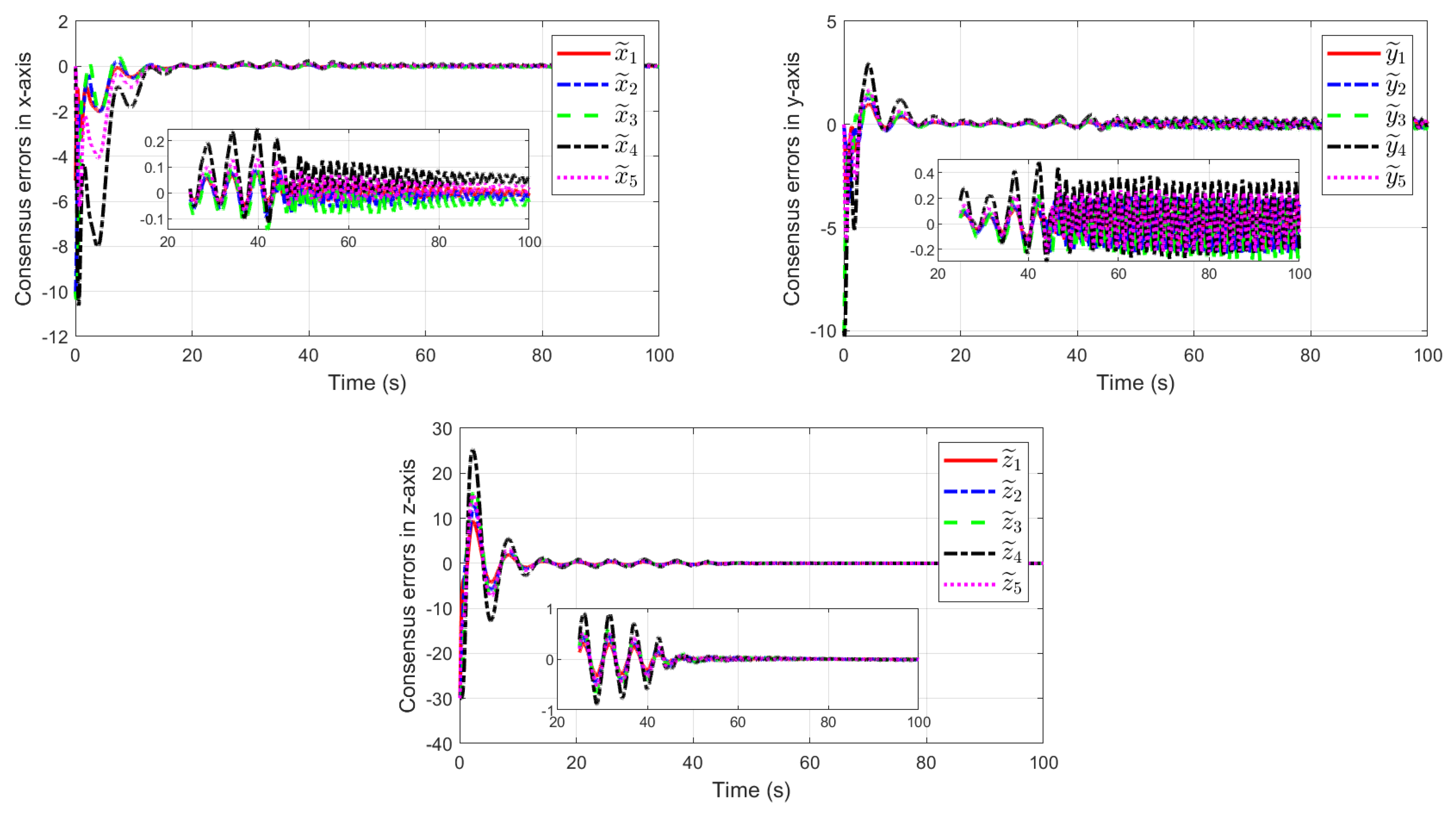
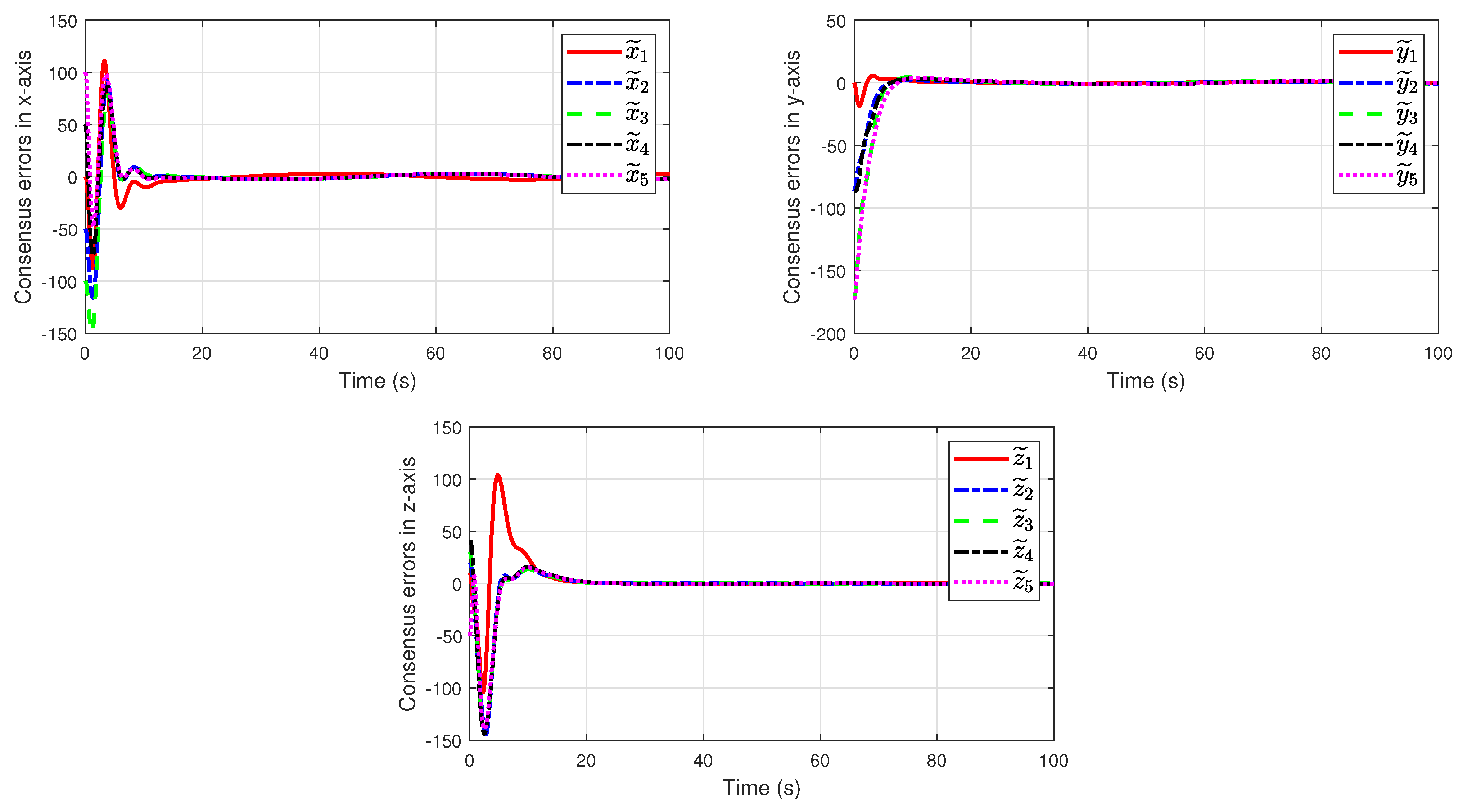
4. Numerical Simulations

A fixed-wing UAV swarm consisting of five members is employed to verify the performance of the presented control strategy. Figure 2 describes the directed topology of a fixed-wing UAV swarm relative to the virtual leader, where 1–5 stand for five members and 0 represents the virtual leader.

To describe the directed topology, one obtains

$$\begin{array}{ccc}& & \mathcal{A}=\left[\begin{array}{ccccc}0& 0& 0& 0& 1\\ 1& 0& 0& 0& 0\\ 0& 1& 0& 0& 0\\ 0& 0& 1& 0& 0\\ 0& 0& 0& 1& 0\end{array}\right],\mathcal{B}=\left[\begin{array}{ccccc}1& 0& 0& 0& 0\\ 0& 0& 0& 0& 0\\ 0& 0& 0& 0& 0\\ 0& 0& 0& 0& 0\\ 0& 0& 0& 0& 0\end{array}\right].\hfill \end{array}$$

The weight of each UAV member is $m_i=5$ kg, gravity acceleration $g=9.81\mathrm{m}/{\mathrm{s}}^2$. The drag force is formulated as [31]

$$\begin{array}{c}\hfill D_i=0.5\rho {({\upsilon }_i-{\overline{\upsilon }}_i)}^2{s}_i{C}_{D0}+\frac{2k_d{k}_n^2{n}_i^2{m}_i^2}{\rho {({\upsilon }_i-{\overline{\upsilon }}_i)}^2{s}_i},\end{array}$$

where the zero-lift drag coefficient and induced drag coefficient are $C_{D0}=0.02$ and $k_d=0.1$, respectively; atmospheric density is $\rho =1.225\mathrm{kg}/{\mathrm{m}}^3$; wing area is $s_i=1.37{\mathrm{m}}^2$; and load-factor effectiveness is $k_n=1$. The gust model ${\overline{\upsilon }}_i=0.215{\upsilon }_m{\log }_{10}\left(h_i\right)+0.285{\upsilon }_m$ with ${\upsilon }_m=4\mathrm{m}/\mathrm{s}$. $\Delta D_i=0.1sin\left(t\right)$, $Y_i=0.1cos\left(t\right)$, $\Delta Y_i=0.01sin\left(t\right)$, $\Delta L_i=0.1sin\left(t\right)$.

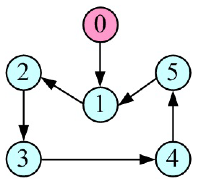
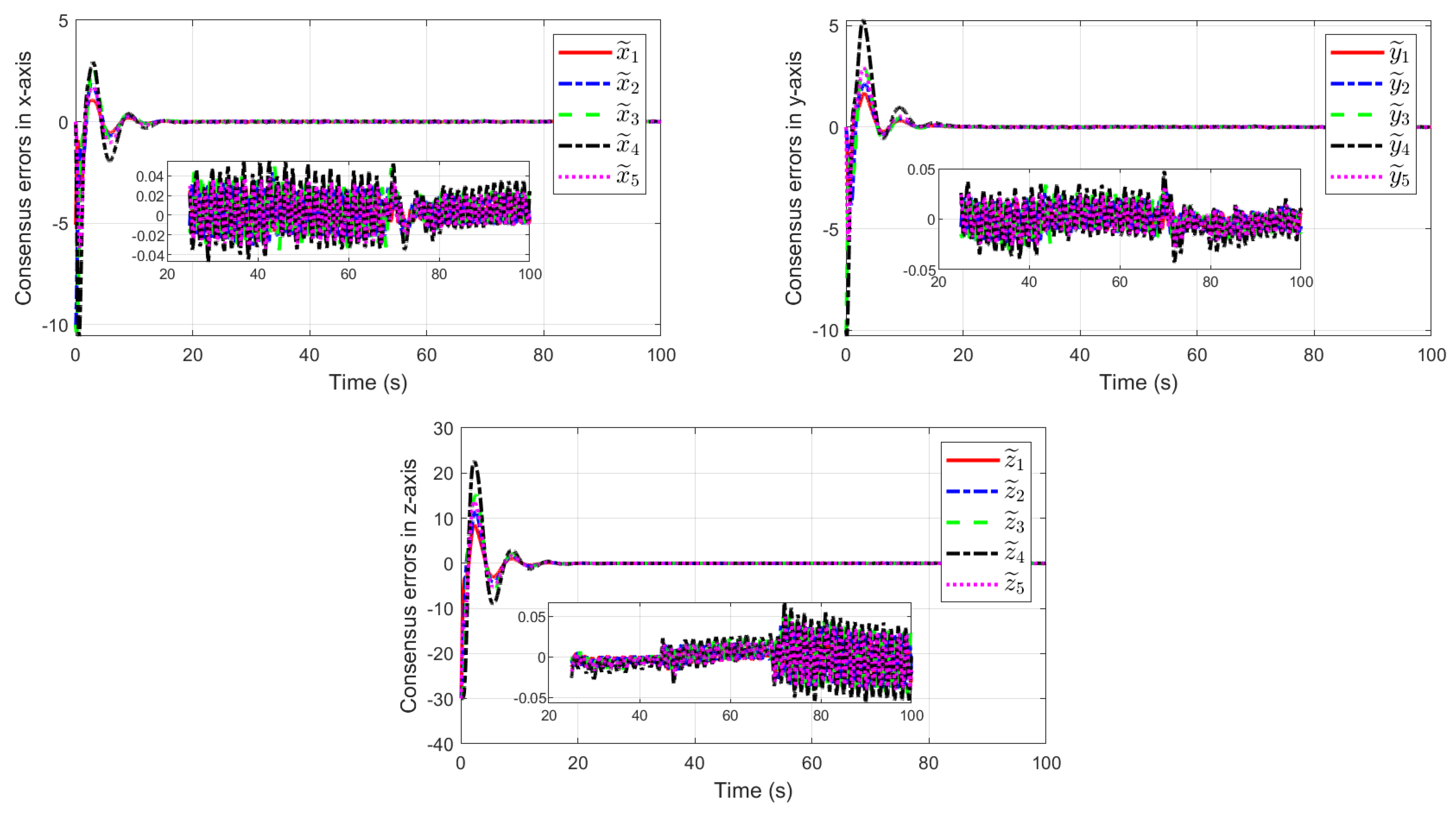
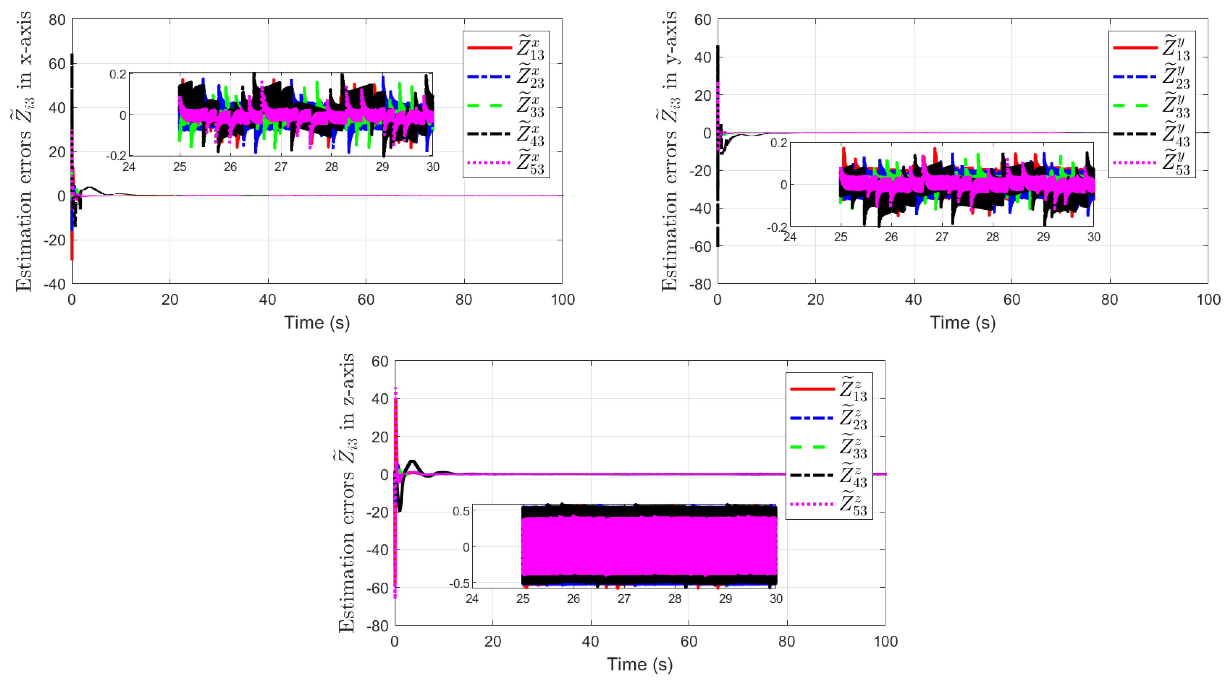
4.1. UAVs Consensus Collaborative Control Scenario

The multiple fixed-wing UAVs consensus collaborative control scenario is simulated. The position and velocity vectors of the virtual leader are set as $X_{01}\left(0\right)=(5,5,80)$ m and $X_{02}\left(0\right)=(3,3,0)$ m/s, respectively. The initial position vectors of five UAV members are

$$X_{11}\left(0\right)=(0,5,50) \mathrm{m},X_{21}\left(0\right)=(-5,5,50) \mathrm{m},$$

$$X_{31}\left(0\right)=(-5,-5,50) \mathrm{m},X_{41}\left(0\right)=(5,-5,50) \mathrm{m},$$

$$X_{51}\left(0\right)=(5,5,50) \mathrm{m},X_{i2}\left(0\right)=(0,0,0) \mathrm{m}/\mathrm{s}.$$

To achieve the state consensus of these fixed-wing UAVs, the parameters of the distributed finite-time ESO (7) and ETM (11) are chosen as ${\beta }_{i1}=100\mathrm{diag}\left\{1,1,1\right\}$, ${\beta }_{i2}=2000\mathrm{diag}\left\{1,1,1\right\}$, ${\beta }_{i3}=600\mathrm{diag}\left\{1,1,1\right\}$, ${\alpha }_1=0.3$, ${\alpha }_2=0.3$, ${\alpha }_3=0.4$, ${\alpha }_4=0.3$, ${\alpha }_5=0.4$; ${\phi }_i=0.2$, ${\delta }_i=0.01$. The gain parameters of the distributed anti-disturbance controller (33) are given as $k_{i1}=\mathrm{diag}\left\{-4,-4,-4\right\}$ and $k_{i2}=\mathrm{diag}\left\{-3,-3,-3\right\}$.

The numerical simulation results are represented in Figure 3 and Figure 4. Specifically, Figure 3 displays the UAV members’ consensus error components relative to the virtual leader. The estimation errors of the total disturbances in the x, y, and z-axis are displayed in Figure 4.

To further illustrate the effectiveness of the inter-trigger output predictor (8) in the proposed methodology, ZOH is used to replace the predictor, namely

$$\begin{array}{c}\hfill {\Pi }_i\left(t\right)=\left\{\begin{array}{c}{\Xi }_{i1}\left(t_k\right),E{T}_i\left(t\right)=0,\hfill \\ {\Xi }_{i1}\left(t\right),E{T}_i\left(t\right)=1.\hfill \end{array}\right.\end{array}$$

(40)

Figure 5 and Figure 6 represent the numerical simulation results using ZOH (40). Thereinto, the consensus errors of each fixed-wing UAV relative to the virtual leader in the x, y, and z-axis are displayed in Figure 5. Figure 6 depicts the estimation errors of the total disturbances in the x, y, and z-axis.

Moreover, a linear ESO is adopted to reflect the advantages of the provided finite-time ESO, which is designed as

$$\begin{array}{cc}\hfill & {\dot{Z}}_{i1}\left(t\right)=Z_{i2}\left(t\right)-{\beta }_{i1}\left(Z_{i1}\left(t\right)-{\Pi }_i\left(t\right)\right),\hfill \end{array}$$

(41a)

$$\begin{array}{cc}\hfill & {\dot{Z}}_{i2}\left(t\right)=Z_{i3}\left(t\right)-{\beta }_{i2}\left(Z_{i1}\left(t\right)-{\Pi }_i\left(t\right)\right)+U_i\left(t\right),\hfill \end{array}$$

(41b)

$$\begin{array}{cc}\hfill & {\dot{Z}}_{i3}\left(t\right)=-{\beta }_{i3}\left(Z_{i1}\left(t\right)-{\Pi }_i\left(t\right)\right).\hfill \end{array}$$

(41c)

The simulation results using a linear ESO are shown in Figure 7 and Figure 8. In Figure 7, the consensus errors of each fixed-wing UAV relative to the virtual leader in the x, y, and z-axis are given. The estimation errors of total disturbances in the x, y, and z-axis are displayed in Figure 8, respectively.

To further compare the control performances,

Table 1. Comparison of the control performance using three methods.

Method	Performance Index
	Convergence Time	$\Theta$	${\Gamma }_{\mathbf{1}}$	${\Gamma }_{\mathbf{2}}$	${\Gamma }_{\mathbf{3}}$	Triggered Ratio (%)
1	15 s	$0.6740$	$0.8524$	$0.8881$	$1.9457$	$52.24$
2	45 s	$0.8882$	$1.5116$	$1.1287$	$2.4328$	$72.78$
3	>100 s	$3.2257$	$2.1567$	$3.2697$	$1.9734$	$91.35$

Method 1: Inter-trigger output predictor-based distributed finite-time ESO; Method 2: ZOH-based distributed finite-time ESO; Method 3: Inter-trigger output predictor-based linear distributed ESO.

displays the simulation results using three of the aforementioned methods. Note that the convergence time describes the speed at which the response curve enters the steady-state range of $\pm 5\%$; meanwhile the averaged consensus error and estimation error are, respectively, defined as

$$\begin{array}{c}\hfill \Theta =\frac{1}{n}\sum _{i=1}^n\sqrt{{\tilde{X}}_{i1}^T\left(t\right){\tilde{X}}_{i1}\left(t\right)/N},{\Gamma }_j=\frac{1}{n}\sum _{i=1}^n\sqrt{{\tilde{Z}}_{ij}^T\left(t\right){\tilde{Z}}_{ij}\left(t\right)/N},\end{array}$$

where $n=5$ and $j=1,2,3$. Clearly, the simulation results reveal that a favorable performance can be obtained by the developed control strategy for the virtual leader-based consensus of a fixed-wing UAV swarm subject to external nonlinear disturbances.

4.2. UAVs Formation Flying Scenario

In this subsection, a fixed-wing UAV swarm formation scenario is simulated. The virtual leader’s desired position vectors is $X_{0d}\left(t\right)=(300sin\left(0.1t\right),100cos\left(0.1t\right),20t)$ m. Figure 9 illustrates the wedge-shaped formation structure of a fixed-wing UAV swarm consisting of five members, whose desired position and velocity vectors are

$$\begin{array}{ccc}& & X_{id}^2\left(t\right)=(0,0,0),X_{1d}^1\left(t\right)=X_{0d}\left(t\right),\hfill \\ & & X_{2d}^1\left(t\right)=X_{0d}\left(t\right)+(L_{d}cos\left({60}^{\circ }\right),L_{d}sin\left({60}^{\circ }\right),0),\hfill \\ & & X_{3d}^1\left(t\right)=X_{0d}\left(t\right)+(2L_{d}cos\left({60}^{\circ }\right),2L_{d}sin\left({60}^{\circ }\right),0),\hfill \\ & & X_{4d}^1\left(t\right)=X_{0d}\left(t\right)+(-L_{d}cos\left({60}^{\circ }\right),L_{d}sin\left({60}^{\circ }\right),0),\hfill \\ & & X_{5d}^1\left(t\right)=X_{0d}\left(t\right)+(-2L_{d}cos\left({60}^{\circ }\right),2L_{d}sin\left({60}^{\circ }\right),0),\hfill \end{array}$$

where $L_d=100$ m. To achieve the wedge-shaped formation flying of multiple fixed-wing UAVs, the distributed anti-disturbance controller is devised as

$$\begin{array}{c}\hfill U_i\left(t\right)=k_{i1}\left(Z_{i1}\left(t\right)-X_{id}^1\left(t\right)\right)+k_{i2}\left(Z_{i2}\left(t\right)-X_{id}^2\left(t\right)\right)-Z_{i3}\left(t\right),\end{array}$$

(42)

where $k_{i1}=diag\left\{-1.2,-1.2,-1,2\right\}$ and $k_{i2}=diag\left\{-2.5,-2.5,-2.5\right\}$.

The UAV members’ trajectories are depicted in Figure 10. Figure 11 displays the error components in the x, y, and z-axis of five UAV members, and Figure 12 shows the estimation errors of the total disturbances ${\tilde{Z}}_{i3}\left(t\right)$ in the x, y, and z-axis. It can be clearly seen that the developed control strategy performs quite well in the process of achieving a formation flying scenario consisting of five fixed-wing UAVs subjected to external disturbances.

5. Conclusions

This paper investigates the coordinated formation flying problem for a fixed-wing UAV swarm considering both internal nonlinearities and external disturbances. A novel distributed finite-time ESO has been put forward based on both ETM and inter-trigger output predictors, where the finite time high-precision estimation of disturbances has been achieved using less communication information. A finite-time ESO-based distributed composite controller has been introduced to guarantee the ultimate bounded stability of the consensus error dynamics. The feasibility of the developed coordinated formation control strategy has been verified via two illustrative numerical simulations, including multiple fixed-wing UAV consensus collaborative control scenarios and formation flying scenarios. Future work will focus on the design of the coordinated formation control scheme for fixed-wing UAVs subject to practical disturbances from other air traffic participants, such as communication jamming and network attacks.

References

1. He, X.; Li, Z.; Wang, X.; Geng, Z. Roto-translation invariant formation of fixed-wing UAVs in 3D: Feasibility and control. Automatica 2024, 161, 111492. [Google Scholar] [CrossRef]
2. Yang, L.; Wang, X.; Zhou, Y.; Liu, Z.; Shen, L. Online predictive visual servo control for constrained target tracking of fixed-wing unmanned aerial vehicles. Drones 2024, 8, 136. [Google Scholar] [CrossRef]
3. Song, B.D.; Park, K.; Kim, J. Persistent UAV delivery logistics: MILP formulation and efficient heuristic. Comput. Ind. Eng. 2018, 120, 418–428. [Google Scholar] [CrossRef]
4. Baniasadi, P.; Foumani, M.; Smithmiles, K.; Ejov, V. A transformation technique for the clustered generalized traveling salesman problem with applications to logistics. Eur. J. Oper. Res. 2020, 285, 444–457. [Google Scholar] [CrossRef]
5. Yan, J.; Yu, Y.; Wang, X. Distance-based formation control for fixed-wing UAVs with input constraints: A low gain method. Drones 2022, 6, 159. [Google Scholar] [CrossRef]
6. Li, Y.; Hua, C.; Guan, X. Distributed output feedback leader-following control for high-order nonlinear multiagent system using dynamic gain method. IEEE Trans. Cybern. 2020, 50, 640–649. [Google Scholar] [CrossRef]
7. Zhang, D.; Duan, H.; Zeng, Z. Leader-follower interactive potential for target enclosing of perception-limited UAV groups. IEEE Syst. J. 2022, 16, 856–867. [Google Scholar] [CrossRef]
8. Wang, W.; Mengali, G.; Quartaand, A.A.; Yuan, J. Distributed adaptive synchronization for multiple spacecraft formation flying around lagrange point orbits. Aerosp. Sci. Technol. 2018, 74, 93–103. [Google Scholar] [CrossRef]
9. Wang, W.; Quarta, A.A.; Mengali, G.; Yuan, J. Multiple solar sail formation flying around heliocentric displaced orbit via consensus. Acta Astronaut. 2019, 154, 256–267. [Google Scholar] [CrossRef]
10. Wu, Y.; Gou, J.; Hu, X.; Huang, Y. A new consensus theory-based method for formation control and obstacle avoidance of UAVs. Aerosp. Sci. Technol. 2020, 107, 106332. [Google Scholar] [CrossRef]
11. Muslimov, T.Z.; Munasypov, R.A. Consensus-based cooperative control of parallel fixed-wing UAV formations via adaptive backstepping. Aerosp. Sci. Technol. 2021, 109, 106416. [Google Scholar] [CrossRef]
12. Zhou, D.; Wang, Z.; Schwager, M. Agile coordination and assistive collision avoidance for quadrotor swarms using virtual structures. IEEE Trans. Robot. 2018, 34, 916–923. [Google Scholar] [CrossRef]
13. Wei, L.; Chen, M.; Li, T. Disturbance-observer-based formation-containment control for UAVs via distributed adaptive event-triggered mechanisms. J. Frankl. Inst. 2021, 358, 5305–5333. [Google Scholar] [CrossRef]
14. Du, Z.; Qu, X.; Shi, J.; Lu, J. Formation control of fixed-wing UAVs with communication delay. ISA Trans. 2024, 146, 154–164. [Google Scholar] [CrossRef] [PubMed]
15. Huang, Z.; Chen, M. Augmented disturbance observer-based appointed-time tracking control of UAVs under exogenous disturbance. IEEE Trans. Intell. Veh. 2024, 9, 2822–2835. [Google Scholar] [CrossRef]
16. Qin, B.; Zhang, D.; Tang, S.; Xu, Y. Two-layer formation-containment fault-tolerant control of fixed-wing UAV swarm for dynamic target tracking. J. Syst. Eng. Electron. 2023, 34, 1375–1396. [Google Scholar] [CrossRef]
17. Liang, Y.; Dong, Q.; Zhao, Y. Adaptive leader-follower formation control for swarms of unmanned aerial vehicles with motion constraints and unknown disturbances. Chin. J. Aeronaut. 2020, 33, 2972–2988. [Google Scholar] [CrossRef]
18. Chen, Q.; Wang, T.; Jin, Y.; Wang, Y.; Qian, B. A UAV formation control method based on sliding-mode control under communication constraints. Drones 2023, 7, 231. [Google Scholar] [CrossRef]
19. Zhi, Y.; Liu, L.; Guan, B.; Wang, B.; Cheng, Z.; Fan, H. Distributed robust adaptive formation control of fixed-wing UAVs with unknown uncertainties and disturbances. Aerosp. Sci. Technol. 2022, 126, 107600. [Google Scholar] [CrossRef]
20. Yu, Z.; Zhang, Y.; Jiang, B.; Su, C.Y.; Chai, T. Fractional-order adaptive fault-tolerant synchronization tracking control of networked fixed-wing UAVs against actuator-sensor faults via intelligent learning mechanism. IEEE Trans. Neural Netw. Learn. Syst. 2021, 32, 5539–5553. [Google Scholar] [CrossRef]
21. Bandyopadhyay, S.; Qin, Z.; Bauer, P. Decoupling control of multi-active bridge converters using linear active disturbance rejection. IEEE Trans. Ind. Electron. 2021, 68, 10688–10698. [Google Scholar] [CrossRef]
22. Chang, S.; Wang, Y.; Zuo, Z. Fixed-time active disturbance rejection control and its application to wheeled mobile robots. IEEE Trans. Syst. Man Cybern. Syst. 2021, 51, 7120–7130. [Google Scholar] [CrossRef]
23. Qin, B.; Yan, H.; Zhang, H.; Wang, Y.; Yang, S. Enhanced reduced-order extended state observer for motion control of differential driven mobile robot. IEEE Trans. Cybern. 2023, 53, 1299–1310. [Google Scholar] [CrossRef] [PubMed]
24. Lu, X.; Li, Z.; Xu, J. Design and control of a hand-launched fixed-wing unmanned aerial vehicle. IEEE Trans. Ind. Inf. 2023, 19, 3006–3016. [Google Scholar] [CrossRef]
25. Yu, Z.; Yang, Z.; Sun, P.; Zhang, Y.; Jiang, B.; Su, C.-Y. Refined fault tolerant tracking control of fixed-wing UAVs via fractional calculus and interval type-2 fuzzy neural network under event-triggered communication. Inf. Sci. 2023, 644, 119276. [Google Scholar] [CrossRef]
26. Zhang, B.; Sun, X.; Liu, S.; Lv, M.; Deng, X. Event-triggered adaptive fault-tolerant synchronization tracking control for multiple 6-DOF fixed-wing UAVs. IEEE Trans. Veh. Technol. 2022, 71, 148–161. [Google Scholar] [CrossRef]
27. Zhang, B.; Sun, X.; Lv, M.; Liu, S. Distributed coordinated control for fixed-wing UAVs with dynamic event-triggered communication. IEEE Trans. Veh. Technol. 2022, 71, 4665–4676. [Google Scholar] [CrossRef]
28. Zhang, Q.; Zhao, D.; Zhu, Y. Event-triggered H control for continuous-time nonlinear system via concurrent learning. IEEE Trans. Syst. Man Cybern. Syst. 2017, 47, 1071–1081. [Google Scholar] [CrossRef]
29. Yu, H.; Hao, F. Input-to-state stability of integral-based event-triggered control for linear plants. Automatica 2017, 85, 248–255. [Google Scholar] [CrossRef]
30. Yue, D.; Tian, E.; Han, Q.-L. A delay system method for designing event-triggered controllers of networked control systems. IEEE Trans. Autom. Control 2013, 58, 475–481. [Google Scholar] [CrossRef]
31. Wang, J.; Xin, M. Integrated optimal formation control of multiple unmanned aerial vehicles. IEEE Trans. Control Syst. Technol. 2013, 21, 1731–1744. [Google Scholar] [CrossRef]
32. Zhu, Z.; Xia, Y.; Fu, M. Attitude stabilization of rigid spacecraft with finite-time convergence. Int. J. Robust Nonlinear Control 2011, 21, 686–702. [Google Scholar] [CrossRef]
33. Wang, H.; Chen, B.; Lin, C.; Sun, Y.; Wang, F. Adaptive finite-time control for a class of uncertain high-order non-linear systems based on fuzzy approximation. IET Control Theory Appl. 2017, 11, 677–684. [Google Scholar] [CrossRef]
34. Yu, Y.; Yuan, Y.; Yang, H.; Liu, H. A novel event-triggered extended state observer for networked control systems subjected to external disturbances. Int. J. Robust Nonlinear Control 2019, 29, 2026–2040. [Google Scholar] [CrossRef]
Figure 1. Control block diagram of fixed-wing UAVs.
Drones 08 00260 g001
Figure 2. Directed topology of a fixed-wing UAV swarm consisting of five members.
Drones 08 00260 g002
Figure 3. Consensus errors of each fixed-wing UAV with the virtual leader.
Drones 08 00260 g003
Figure 4. Estimation errors of total disturbances.
Drones 08 00260 g004
Figure 5. Consensus errors of each fixed-wing UAV with the virtual leader using ZOH.
Drones 08 00260 g005
Figure 6. Estimation errors of the total disturbances using ZOH.
Drones 08 00260 g006
Figure 7. Consensus errors of each fixed-wing UAV with the virtual leader using linear ESO.
Drones 08 00260 g007
Figure 8. Estimation errors of the total disturbances using linear ESO.
Drones 08 00260 g008
Figure 9. Wedge-shaped formation of a fixed-wing UAV swarm.
Drones 08 00260 g009
Figure 10. Formation flying with wedge-shaped.
Drones 08 00260 g010
Figure 11. Consensus errors of each fixed-wing UAV with the virtual leader using linear ESO.
Drones 08 00260 g011
Figure 12. Estimation errors of the total disturbances using linear ESO.
Drones 08 00260 g012