

Multi-Objective Deployment of UAVs for Multi-Hop FANET: UAV-Assisted Emergency Vehicular Network


Abstract
1. Introduction
- UAVs need to automatically plan a trajectory through the coarse-grained locations of multiple targets in complex environments with obstacles [10]. The trajectory planning method requires the avoidance of collisions with obstacles or other UAVs. It also has the capability to automatically adjust the trajectory by sensing obstacles or using target information.
- The ad hoc network is constructed according to the multi-objective requirements, including a lower arrangement cost, less link interference, and a lower hop count. Considering the requirements of a rapid connection and stable link, the multi-objective network optimum strategy needs to be inserted into the trajectory planning method, rather than implementing optimum adjustment after the network is built. It is undoubtedly going to enhance the difficulty if the UAVs must find a path and construct a link in an unknown environment with little target location information and no obstacle information.
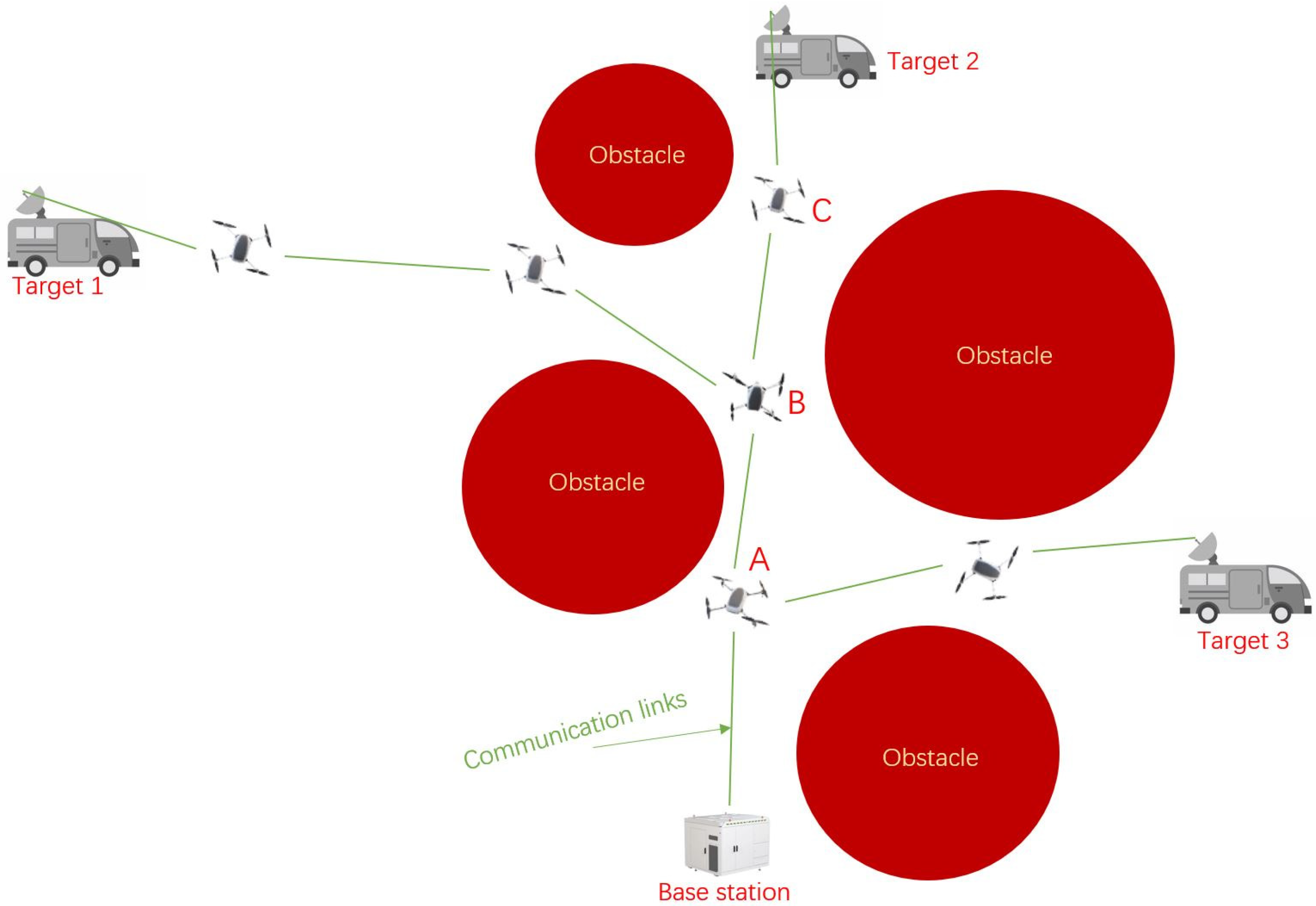
- In the search for multiple targets, parts of multiple paths can overlap; thus, a portion of the relay nodes can be shared to decrease the arrangement costs. The problem transforms into one in which the branching node must be set so that it can decide when and where to separate the common trajectory into multiple paths to different targets [11].
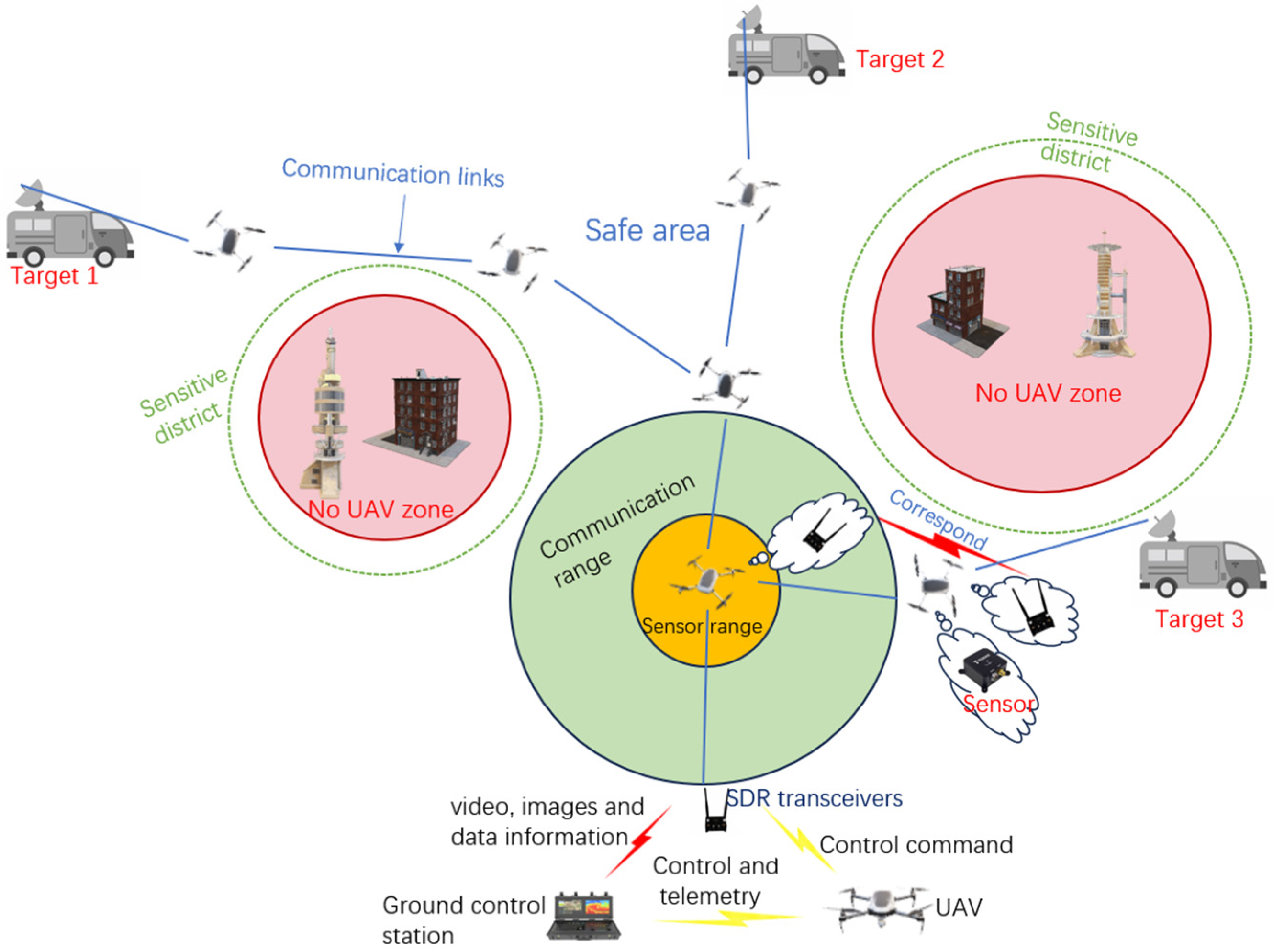
- An intelligent trajectory planning method is presented for searching for trapped vehicles. Each UAV navigates to the cross-point location between the boundary of the last UAV’s maximum communication range and the line to the target. During the navigating process, the UAV implements collision-less movements while sensing the obstacle’s location.
- A multi-objective deployment strategy is presented for the emergency network with a lower arrangement cost, less link interference, and a lower hop count. A multi-objective particle swarm optimization algorithm (MOPSO) is applied to solve this deployment problem [12].
2. Related Works
2.1. Search and Rescue Task in FANET
2.2. The Deployment Optimization in SAR Task
- Static or dynamic deployment. As the static deployment method [18] obtains the geographical location information around the trapped target in advance, it always adopts a centralized decision when arranging to send a suitable UAV to the relay placement area for optimal networking. Conversely, the dynamic deployment method [19] always solves the problems of an unknown environment, which include the unknown obstacle, the unknown trapped target, and even an uncertain searching region. Thus, it always adopts a distributed decision to make the UAV implement a series of actions that involve sensing, finding a pathway, searching for a target, and obstacle avoidance. After receiving a round of information, the UAVs collaborate to make an action decision in the next round.
- Single or multiple targets. In the single-target SAR task, the deployment method only considers the shortest path to connect the existing base station to the trapped target without obstacles. However, in the multi-target SAR task, the deployment method simultaneously takes two factors into account. The first is the choice of multiplexed nodes. A higher number of multiplexed nodes means less placement cost and easier destructibility. The second one is related to the large search span in dynamic deployment. The temporary network searching process can guarantee the synchronization of each round of information; consequently, the search direction is adjusted in a timely manner to avoid meaningless migration.
- Single or multiple objectives. In single-objective optimization, the solving method is relatively easy to use when determining the optimal deployment solutions. In multi-objective optimization, the weight combination among the multiple objectives is critical for deciding the performance of the deployment solutions [20]. The manual setup easily transforms the solution into an experienced local optimum. The machine setup may search out multiple solutions, but most of the solutions are difficult to realize because the actual environment has complex and unpredictable constraints.
3. Problem Formulation
3.1. Problem Description
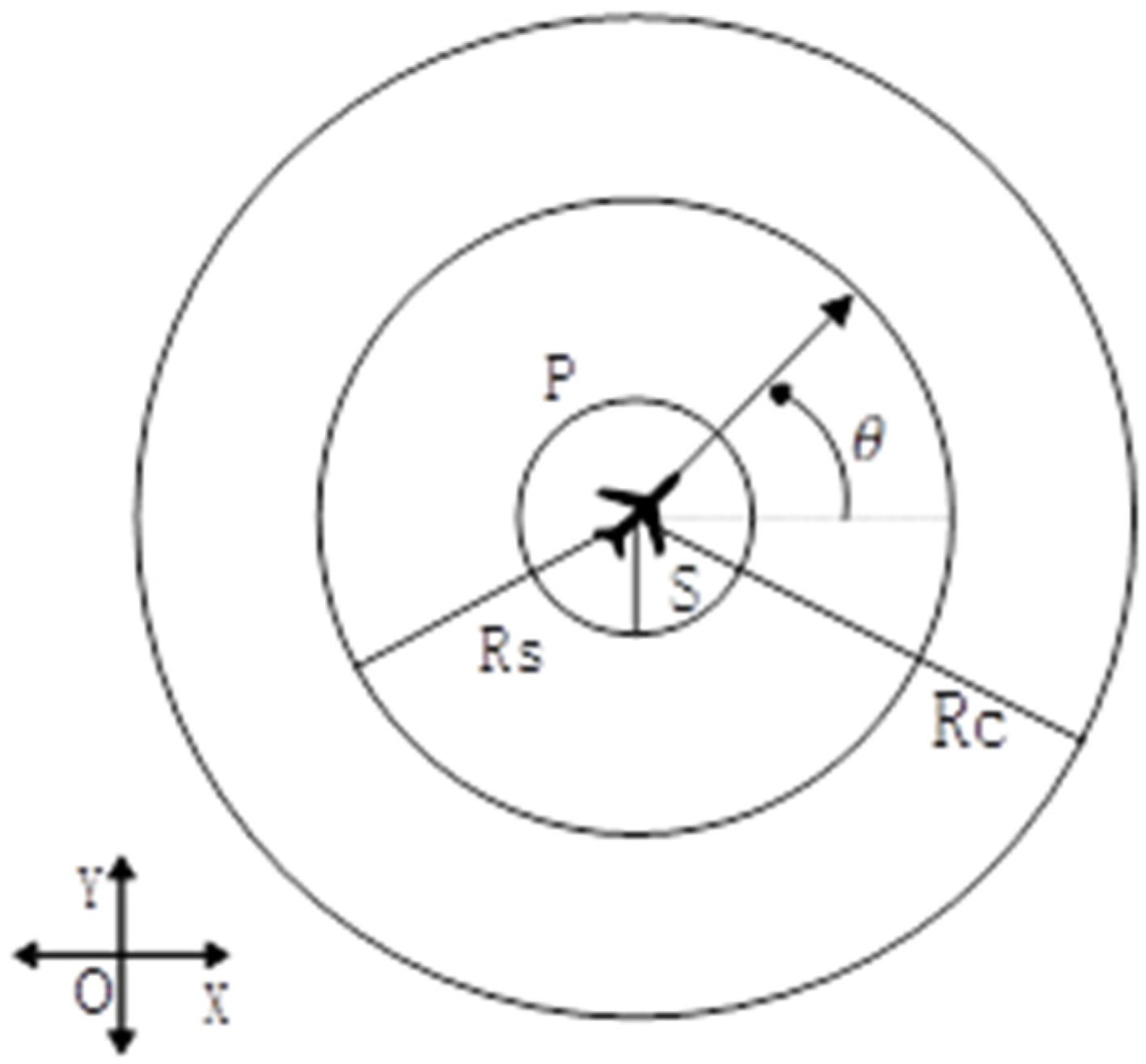
3.1.1. UAV Model
3.1.2. Obstacle Avoidance Model
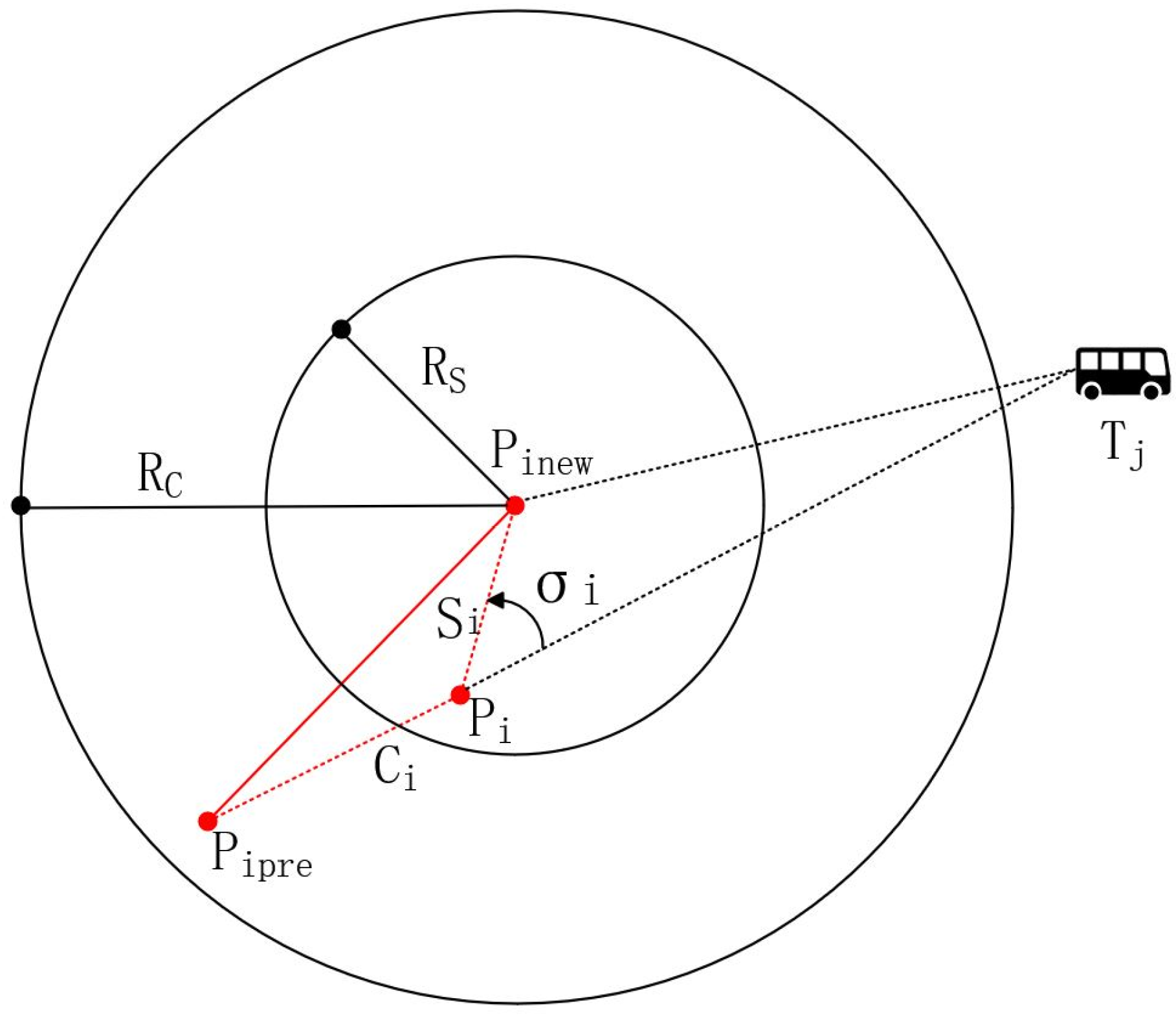
3.1.3. Target Angle Model
3.2. Optimization Indexes
- (1)
- Minimizing the target angle F1:
- (2)
- Optimizing communication links F2:
- (3)
- Optimizing sensing links F3:
- (4)
- Avoiding obstacles F4:
4. The UMMVN Method
4.1. The Framework of UMMVN
4.1.1. MOPSO-Based Trajectory Planning Method
| Algorithm 1. MOPSO-based planning trajectory |
| Input: , and Output: Optimal position 1. Initialize: MOPSO initial population 2. Mapping obstacles in environment into restricted area in the searching region 3. for from 1 to do 4. for Particle in solutions do 5. Calculate cost value of Particle 6. Evaluate Particle ’s priority in terms of four objectives and density 7. Update and 8. Update velocities and positions 9. end 10. end |
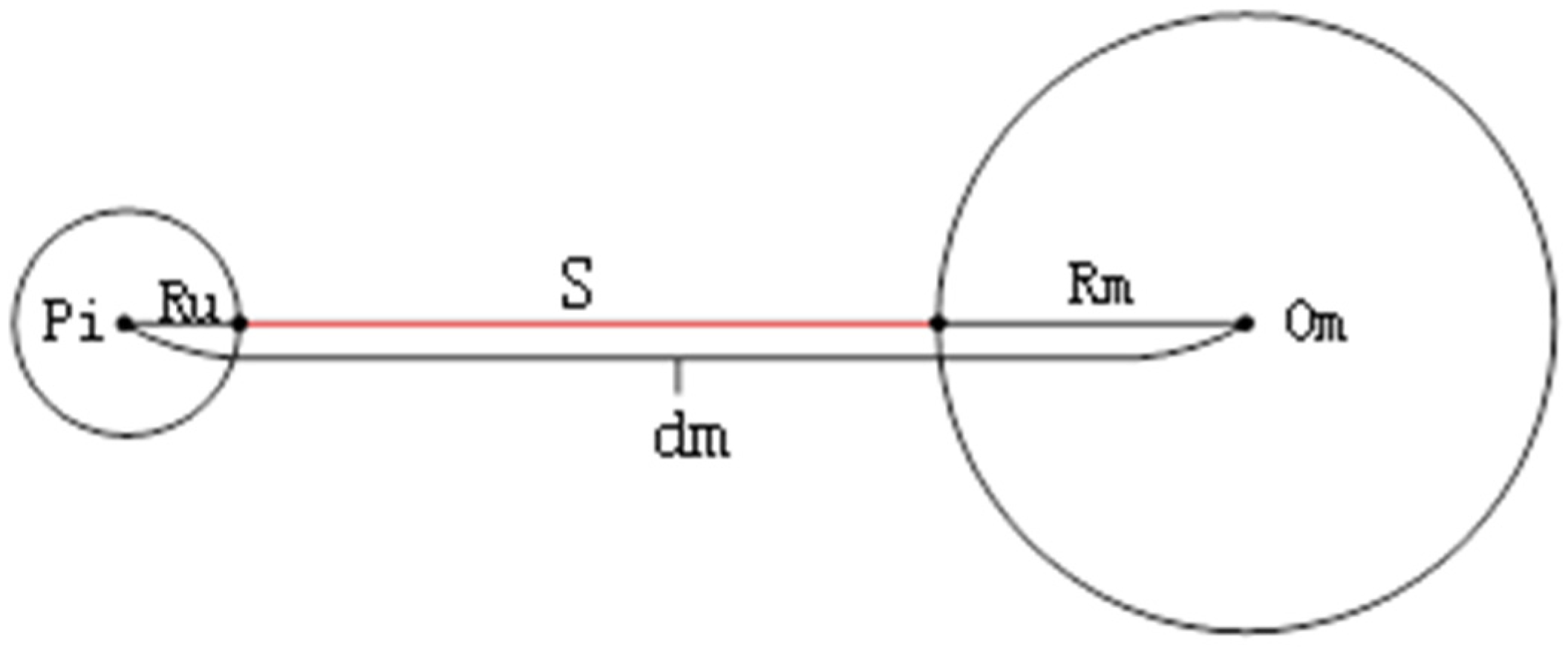
4.1.2. Single-Target Relay Deployment Method
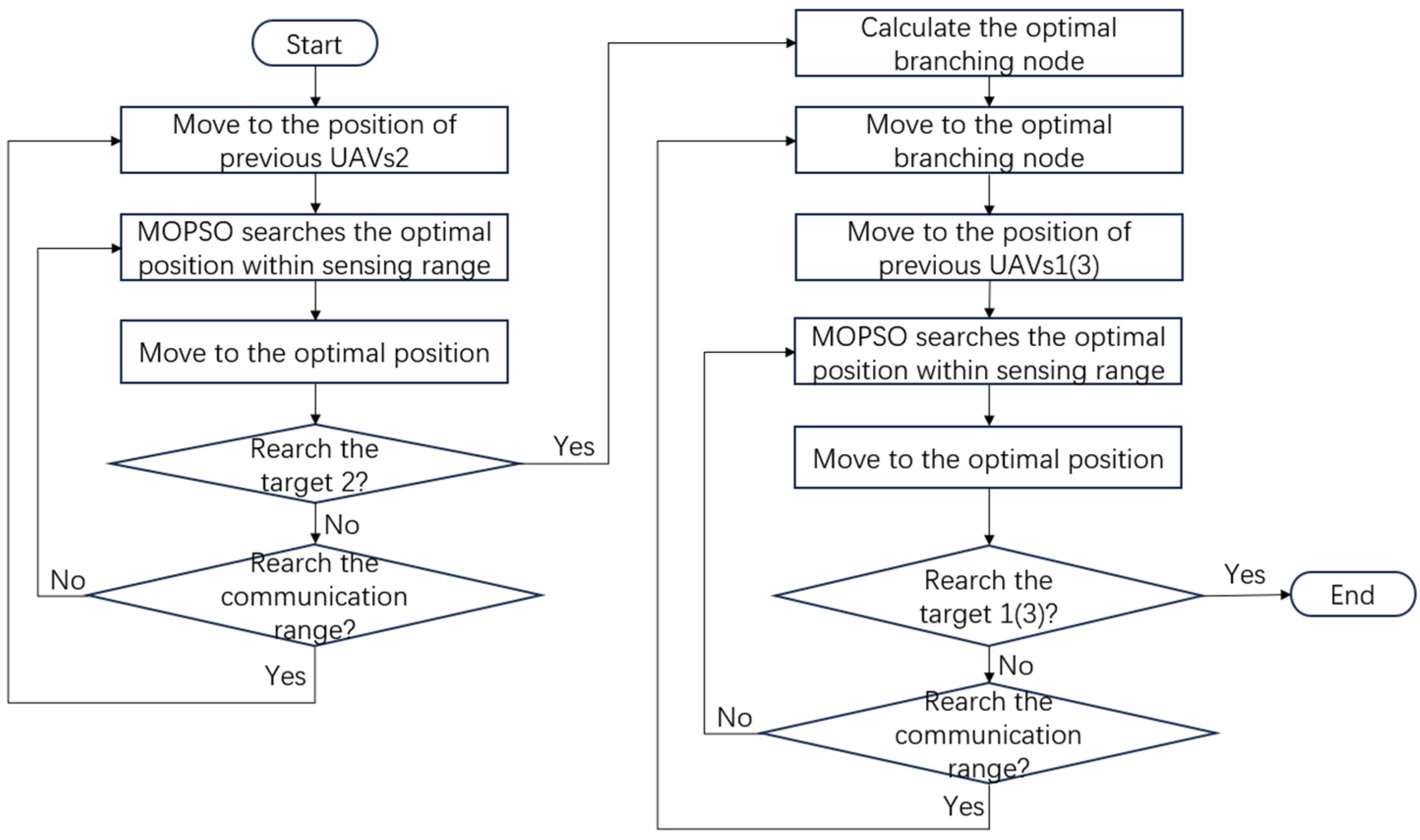
4.1.3. Multi-Target Searching Method
| Algorithm 2. Multi-objective Multi-hop Ad-hoc Communication Route Deployment Strategy |
|
1. Initialization
2. m1: Calculate the distance between the start and the target 1 3. m2: Calculate the distance between the start and the target 3 4. minimum_distance1 = m1 5. minimum_distance2 = m2 6. Single objective multi-hop ad-hoc communication route deployment of UAVs2 to target 2 7. Record the position of the UAVs2 8. for i = 1:end 9. d1: Calculate the distance between the UAVs2(i) and target 1 10. d2: Calculate the distance between the UAVs2(i) and target 3 11. if d1 < minimum_distance1 12. minimum_distance1 = d1 13. P1 = the position of the UAVs2(i) 14. end 15. if minimum_distance1==m1 16. P1 = start 17. end 18. if d2 < minimum_distance2 19. minimum_distance2 = d2 20. P2 = the position of the UAVs2(i) 21. end 22. if minimum_distance2==m2 23. P2 = start 24. end 25. end 26. While not reach target 1 27. UAVs1(j) moves to P1 28. Single objective multi-hop ad-hoc communication route deployment of UAVs1 to target 1 29. end 30. While not reach target 3 31. UAVs3(k) moves to P2 32. Single objective multi-hop ad-hoc communication route deployment of UAVs3 to target 3 33. end |
4.2. Optimal Branching Node Strategy
4.3. Searching Algorithm
4.3.1. MOPSO Algorithm
4.3.2. NSGA2 Algorithm
4.3.3. Algorithm Comparison
- (1)
- Optimization method:
- (2)
- Iteration method:
5. Experiment
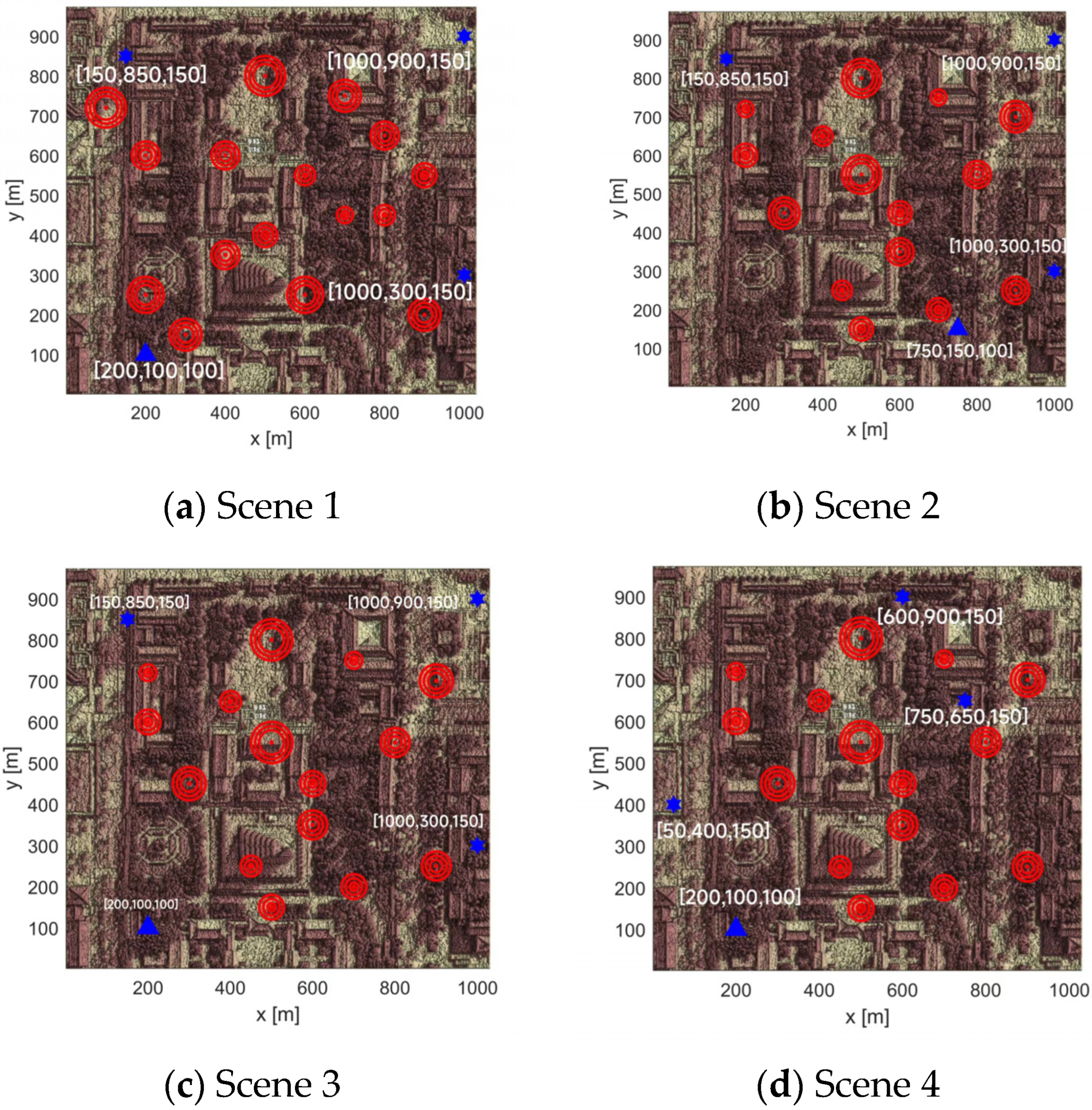
5.1. Experiment Setup
5.2. Experiments Results
- (1)
- MOPSO search optimal time: The sensing range of the UAV was 60 m, and the flight speed was set to 20 m/s. Therefore, it took 3 s for the UAV to fly from the optimal point to the latest searched optimal point. From the perspective of iteration and search time, its search time was within 1 s, ensuring real-time performance.
- (2)
- Link length between UAVs: According to the data, the distance between every two UAVs was less than 360 m, indicating that they could communicate normally. The average intermediate link length was around 355 m, which was close to 360 m. Therefore, fewer UAVs were required, which reduced the costs.
- (3)
- Total link length: According to the data, the difference between the total ideal link length and the actual link length was relatively small. Within an acceptable range, the reason for the error was due to the presence of obstacles. However, it was found in some of the data that the actual link length was smaller than the ideal link length. This was because the target point reached by the UAV during the flight deviated from the actual target point, resulting in this situation.
5.3. Comparative Analysis of Algorithm Performance
5.3.1. Indicator Values
5.3.2. Performance Analysis
6. Conclusions
Author Contributions
Funding
Data Availability Statement
Conflicts of Interest
References
- Prakash, J.; Murali, L.; Manikandan, N.; Nagaprasad, N.; Ramaswamy, K. A vehicular network based intelligent transport system for smart cities using machine learning algorithms. Sci. Rep. 2024, 14, 468. [Google Scholar] [CrossRef] [PubMed]
- Hayat, S.; Yanmaz, E.; Muzaffar, R. Survey on Unmanned Aerial Vehicle Networks for Civil Applications: A Communications Viewpoint. IEEE Commun. Surv. Tutor. 2016, 18, 2624–2661. [Google Scholar] [CrossRef]
- Thuy, N.D.T.; Bui, D.N.; Phung, M.D.; Duy, H.P. Deployment of UAVs for Optimal Multihop Ad-hoc Networks Using Particle Swarm Optimization and Behavior-based Control. In Proceedings of the 2022 11th International Conference on Control, Automation and Information Sciences (ICCAIS), Hanoi, Vietnam, 21–24 November 2022; pp. 304–309. [Google Scholar] [CrossRef]
- Lee, H.; Zhu, Y.; Wapenski, D.; Wang, X.; Zhang, Q.; Palacharla, P.; Ikeuchi, T. A Stochastic Process based Routing Algorithm for Wireless Ad Hoc Networks. In Proceedings of the 2019 International Conference on Computing, Networking and Communications (ICNC), Honolulu, HI, USA, 18–21 February 2019; pp. 1018–1023. [Google Scholar] [CrossRef]
- Wang, D.; Wu, M.; Chakraborty, C.; Min, L.; He, Y.; Guduri, M. Covert Communications in Air-ground Integrated Urban Sensing Networks Enhanced by Federated Learning. IEEE Sens. J. 2023, 24, 5636–5643. [Google Scholar] [CrossRef]
- Wang, H.; Zhao, H.; Zhou, L.; Ma, D.; Wei, J. Deployment algorithm for minimum unmanned aerial vehicles towards optimal coverage and interconnections. In Proceedings of the 2018 IEEE Wireless Communications and Networking Conference Workshops (WCNCW), Barcelona, Spain, 15–18 April 2018; pp. 72–277. [Google Scholar] [CrossRef]
- Yu, P.; Ding, Y.; Li, Z.; Tian, J.; Zhang, J.; Liu, Y.; Li, W.; Qiu, X. Energy-Efficient Coverage and Capacity Enhancement with Intelligent UAV-BSs Deployment in 6G Edge Networks. IEEE Trans. Intell. Transp. Syst. 2023, 24, 7664–7675. [Google Scholar] [CrossRef]
- Chao, D. A survey of UAV-based edge intelligent computing. Chin. J. Intell. Sci. Technol. 2020, 2, 227–239. [Google Scholar] [CrossRef]
- Masroor, R.; Naeem, M.; Ejaz, W. Efficient deployment of UAVs for disaster management: A multi-criterion optimization approach. Comput. Commun. 2021, 177, 185–194. [Google Scholar] [CrossRef]
- Wang, D.; Wu, M.; Wei, Z.; Yu, K.; Min, L.; Mumtaz, S. Uplink Secrecy Performance of RIS-based RF/FSO Three-Dimension Heterogeneous Networks. IEEE Trans. Wirel. Commun. 2023, 23, 1798–1809. [Google Scholar] [CrossRef]
- Liang, J.; Huang, X.; Xu, Q.; Liu, Y.; Zhang, J.; Huang, J. A Novel UAV-Assisted Multi-Mobility Channel Model for Urban Transportation Emergency Communications. Electronics 2023, 12, 3015. [Google Scholar] [CrossRef]
- Pandey, K.K.; Kumbhar, C.; Parhi, D.R.; Mathivanan, S.K.; Jayagopal, P.; Haque, A. Trajectory Planning and Collision Control of a Mobile Robot: A Penalty-Based PSO Approach. Math. Probl. Eng. 2023, 2023, 1040461. [Google Scholar] [CrossRef]
- Khan, M.A.; Qureshi, I.M.; Khanzada, F. A Hybrid Communication Scheme for Efficient and Low-Cost Deployment of Future Flying Ad-Hoc Network (FANET). Drones 2019, 3, 16. [Google Scholar] [CrossRef]
- Liu, W.; Hu, K.; Li, Y.; Liu, Z. A review of prediction methods for moving target trajectories. Chin. J. Intell. Sci. Technol. 2021, 3, 149–160. [Google Scholar]
- Keerthinathan, P.; Amarasingam, N.; Hamilton, G.; Gonzalez, F. Exploring unmanned aerial systems operations in wildfire management: Data types, processing algorithms and navigation. Int. J. Remote Sens. 2023, 44, 5628–5685. [Google Scholar] [CrossRef]
- Wang, X.; Shi, S.; Xue, J.; Wu, C. Controller placement in software defined FANET. Wirel. Networks 2023, 3, 1–14. [Google Scholar] [CrossRef]
- Chriki, A.; Touati, H.; Snoussi, H.; Kamoun, F. FANET: Communication, mobility models and security issues. Comput. Netw. 2019, 163, 106877. [Google Scholar] [CrossRef]
- Lu, H.; Yang, Y.; Tao, R.; Chen, Y. Coverage Path Planning for SAR-UAV in Search Area Coverage Tasks Based on Deep Reinforcement Learning. In Proceedings of the 2022 IEEE International Conference on Unmanned Systems (ICUS), Guangzhou, China, 28–30 October 2022; pp. 248–253. [Google Scholar] [CrossRef]
- Karimi-Bidhendi, S.; Guo, J.; Jafarkhani, H. Energy-Efficient Deployment in Static and Mobile Heterogeneous Multi-Hop Wireless Sensor Networks. IEEE Trans. Wirel. Commun. 2022, 21, 4973–4988. [Google Scholar] [CrossRef]
- Wang, D.; He, T.; Lou, Y.; Pang, L.; He, Y.; Chen, H.-H. Double-edge Computation Offloading for Secure Integrated Space-air-aqua Networks. IEEE Internet Things J. 2023, 10, 15581–15593. [Google Scholar] [CrossRef]


| Scene | UAVs | Link Length (m) | Actual Total Link Length (m) | Ideal Link Length (m) | Temporary Goal Number | Time Consuming (s) | ||
|---|---|---|---|---|---|---|---|---|
| Searching | Searching Time/Temporary Goal (s) | |||||||
| 1 | uavs1 | 1 | 355.2071 | 583.8348 | 588.9528 | 7 | 5.4969 | 0.7853 |
| 2 | 228.6277 | 4 | 3.2112 | 0.8028 | ||||
| uavs2 | 1 | 354.8361 | 1140.155 | 1134.6347 | 7 | 5.6935 | 0.8134 | |
| 2 | 355.3513 | 8 | 7.0538 | 0.8817 | ||||
| 3 | 355.2691 | 7 | 5.4157 | 0.7737 | ||||
| 4 | 74.6985 | 2 | 1.5258 | 0.7629 | ||||
| uavs3 | 1 | 355.5759 | 415.2266 | 400.7387 | 7 | 5.4158 | 0.7737 | |
| 2 | 59.6508 | 1 | 0.74432 | 0.7443 | ||||
| 2 | uavs1 | 1 | 308.0387 | 308.0387 | 304.7666 | 6 | 4.5579 | 0.7597 |
| uavs2 | 1 | 354.9888 | 897.6647 | 894.4725 | 7 | 5.5376 | 0.7911 | |
| 2 | 355.2532 | 8 | 7.2867 | 0.9108 | ||||
| 3 | 187.4227 | 4 | 3.6366 | 0.9092 | ||||
| uavs3 | 1 | 243.4712 | 243.4712 | 231.849 | 5 | 4.0102 | 0.8020 | |
| 3 | uavs1 | 1 | 355.3137 | 566.4317 | 570.6765 | 7 | 5.8619 | 0.8374 |
| 2 | 211.118 | 4 | 3.4564 | 0.8641 | ||||
| uavs2 | 1 | 355.2151 | 1167.4998 | 1143.1955 | 7 | 5.6761 | 0.8109 | |
| 2 | 355.1901 | 7 | 5.8394 | 0.8342 | ||||
| 3 | 355.1351 | 7 | 5.653 | 0.8076 | ||||
| 4 | 101.9595 | 2 | 1.6899 | 0.8450 | ||||
| uavs3 | 1 | 355.272 | 438.801 | 449.6769 | 7 | 5.7628 | 0.8233 | |
| 2 | 83.529 | 2 | 1.7585 | 0.8793 | ||||
| 4 | uavs1 | 1 | 354.2717 | 814.7755 | 807.2607 | 7 | 5.8517 | 0.8360 |
| 2 | 358.7073 | 8 | 7.2191 | 0.9024 | ||||
| 3 | 101.7965 | 2 | 1.6275 | 0.8138 | ||||
| uavs2 | 1 | 355.1346 | 791.1892 | 790.7522 | 7 | 5.7114 | 0.8159 | |
| 2 | 355.3802 | 7 | 5.859 | 0.8370 | ||||
| 3 | 80.6744 | 1 | 0.83004 | 0.8300 | ||||
| uavs3 | 1 | 227.6825 | 227.6825 | 232.0162 | 6 | 4.9498 | 0.8250 | |
| Scene | Target 1 | Target 2 | Target 3 |
|---|---|---|---|
| 1 | 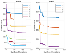 | 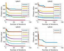 | 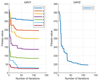 |
| 2 | 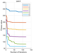 | 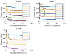 |  |
| 3 | 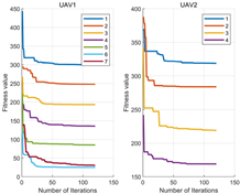 | 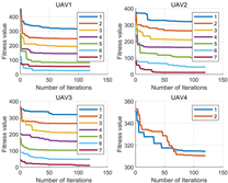 | 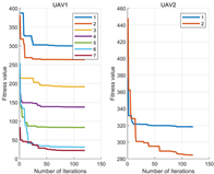 |
| 4 |  |  | 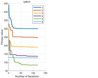 |
| Scene | Uavs 1 | Uavs 2 | Uavs 3 | Average RMSE |
|---|---|---|---|---|
| 1 | 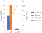 |  | 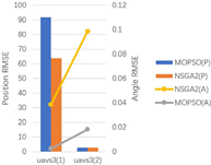 | 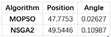 |
| 2 | 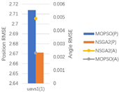 | 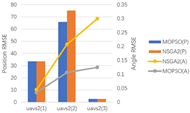 |  |  |
| 3 |  | 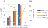 | 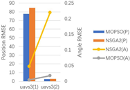 |  |
| 4 | 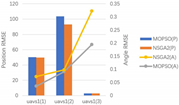 | 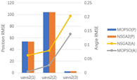 | 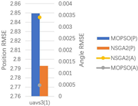 | 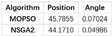 |
| Scene | Uavs 1 | Uavs 2 | Uavs 3 |
|---|---|---|---|
| 1 | 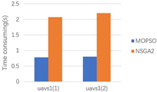 |  | 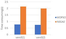 |
| 2 | 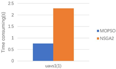 |  |  |
| 3 | 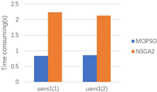 |  |  |
| 4 |  |  | 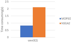 |
Disclaimer/Publisher’s Note: The statements, opinions and data contained in all publications are solely those of the individual author(s) and contributor(s) and not of MDPI and/or the editor(s). MDPI and/or the editor(s) disclaim responsibility for any injury to people or property resulting from any ideas, methods, instructions or products referred to in the content. |
© 2024 by the authors. Licensee MDPI, Basel, Switzerland. This article is an open access article distributed under the terms and conditions of the Creative Commons Attribution (CC BY) license (https://creativecommons.org/licenses/by/4.0/).
Share and Cite
Li, H.; Hao, X.; Wen, J.; Liu, F.; Zhang, Y. Multi-Objective Deployment of UAVs for Multi-Hop FANET: UAV-Assisted Emergency Vehicular Network. Drones 2024, 8, 262. https://doi.org/10.3390/drones8060262
Li H, Hao X, Wen J, Liu F, Zhang Y. Multi-Objective Deployment of UAVs for Multi-Hop FANET: UAV-Assisted Emergency Vehicular Network. Drones. 2024; 8(6):262. https://doi.org/10.3390/drones8060262
Chicago/Turabian StyleLi, Haoran, Xiaoyao Hao, Juan Wen, Fangyuan Liu, and Yiling Zhang. 2024. "Multi-Objective Deployment of UAVs for Multi-Hop FANET: UAV-Assisted Emergency Vehicular Network" Drones 8, no. 6: 262. https://doi.org/10.3390/drones8060262
APA StyleLi, H., Hao, X., Wen, J., Liu, F., & Zhang, Y. (2024). Multi-Objective Deployment of UAVs for Multi-Hop FANET: UAV-Assisted Emergency Vehicular Network. Drones, 8(6), 262. https://doi.org/10.3390/drones8060262