Abstract
This paper investigates the target fencing control problem of fixed-wing Unmanned Aerial Vehicle (UAV) swarms with collision avoidance and connectivity maintenance in obstacle environments. A distributed cooperative fencing scheme for maneuvering targets is proposed without predefined accurate formation. Firstly, considering that not all states of the target can be obtained by UAVs, a differential state observer is developed to estimate the target’s unknown speed and control input. Secondly, by constructing potential functions with fewer parameter adjustments, corresponding negative gradient terms are calculated to guarantee the flight safety and communication connectivity of the swarm. A distributed cooperative controller is designed using the self-organized theory and consensus control. Additionally, the stability of the closed-loop system with the controller is analyzed based on Lyapunov stability theory. Finally, numerical simulations are performed to illustrate the effectiveness of the proposed scheme.
1. Introduction
UAVs have been endowed with stronger autonomous decision-making and response capabilities through artificial intelligence technology. Nevertheless, the intricacy of flight airspace and the constraints of onboard sensors pose challenges for a single UAV in executing complex tasks. The UAV swarm effectively mitigates these limitations by leveraging cooperative capabilities. They are often applied to high-risk and easily exposed tasks such as target tracking [1,2], target fencing [3,4], and area searching [5]. Consequently, they have received widespread attention from scholars [6,7].
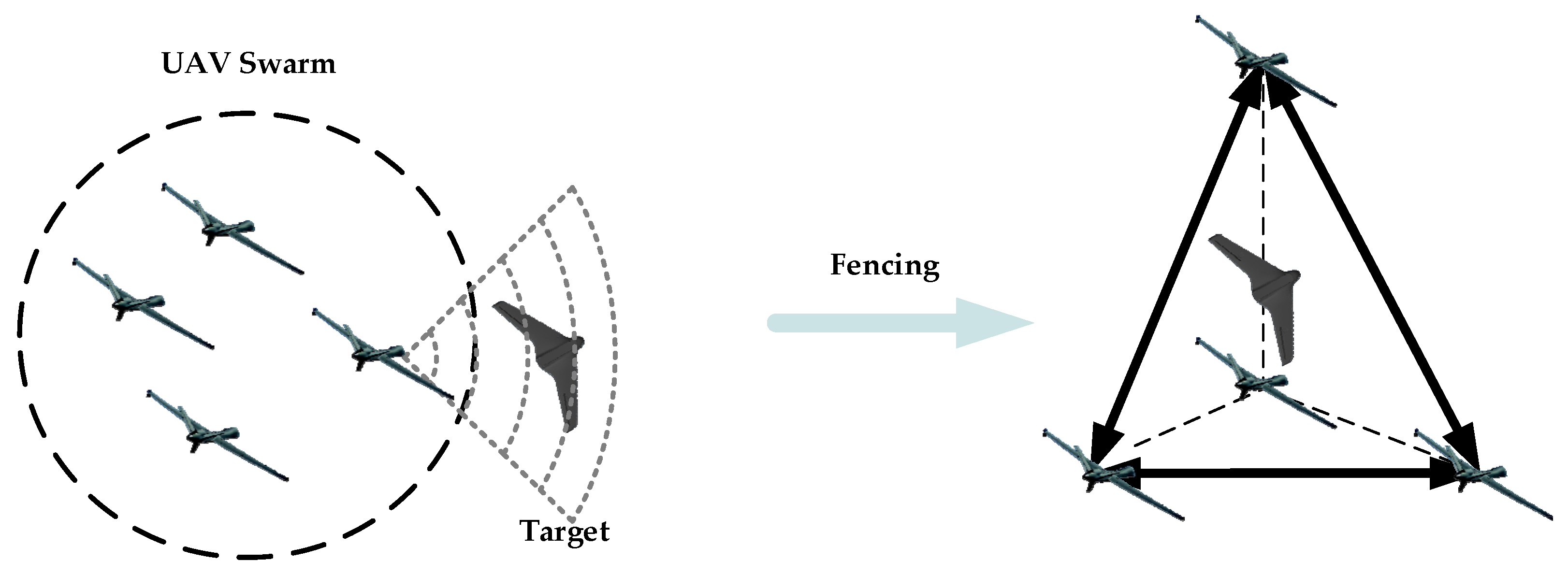
Target fencing control aims to design a cooperative controller for a group of UAVs to enclose the target within their flight convex hull [8]. The design of the fencing strategy focuses on four main aspects. The first aspect involves how to obtain the target’s unknown state. In practical tracking or fencing scenarios, the target is typically uncooperative, implying that its speed and control input are not directly accessible. Several studies assume that the target’s states were partially or entirely known by UAVs. In [9], a high-order sliding mode observer was designed to estimate the unmeasurable linear velocity of the target, enabling UAVs to enclose the target in the desired formation. In [10], the target’s state can be obtained by certain UAVs and transmitted to their neighbors through the network for distributed estimation within each formation form. An adaptive extended state observer was constructed in [11] which can simultaneously estimate the leader’s maneuvers and external disturbances.
The second aspect involves designing an appropriate control scheme for fencing. To address the problem of fencing control, various relevant controllers were designed [12,13,14,15]. In [12], a formation controller was designed to ensure that followers gradually converge to the moving convex hull formed by leaders. Based on a disturbance observer, a formation controller was designed in [13] to achieve fencing control for unmanned surface vehicle swarms containing uncertainty and external disturbance. In [14,15], a distributed circular formation controller was introduced to fence the target by guiding agents toward a fixed-distance circle centered on the target. Most existing fencing control studies, including the aforementioned literature, require pre-designing desired orientations or distances centered around the target. However, in practical applications, defining appropriate parameter values becomes challenging due to complex flight environments of UAV swarms. To overcome this, a cooperative controller for fencing the target with a constant speed was presented in [16], eliminating preset formation parameters. Building upon [16], cooperative controllers for fencing targets were further developed for mobile robot systems and UAV swarms in [17,18].
The third aspect involves the security control of the target fencing process. Safety requirements, including collision avoidance and obstacle avoidance, are fundamental for the successful swarm execution of target fencing, as well as prerequisites for other tasks [19]. Therefore, the problem of swarm cooperative control with a security mechanism is studied. Currently, there exist three methods to ensure swarm security control. The first is the widely used artificial potential field (APF) method [20,21,22,23,24]. In [20], a safety overtaking controller for multi-unmanned ground vehicles in dynamic environments was designed based on APF. In [21], an adaptive controller that combines repulsive potential function and sliding manifold was proposed to achieve the fixed-time convergence of agent formation. To address the secure area control in second-order agent systems, an exponential control obstacle function was introduced in [22] to ensure internal collision avoidance and the external obstacle avoidance of agents. In [23,24], collision avoidance in formation and trajectory tracking were solved based on the consensus term and collision avoidance term, respectively. Additionally, distributed model predictive control (DMPC) also serves as an effective method for ensuring swarm security control. In [25], DMPC was introduced to avoid collision in the formation navigation control of unmanned underwater vehicles. In [26], the MPC method was utilized to eliminate collision risks during the formation reconstruction of the robot system. In [27], a combined soft/hard constraint-based MPC scheme was designed to tackle both collision avoidance and obstacle avoidance challenges encountered by UAV swarms. The stability and feasibility of MPC for collision and obstacle avoidance in multi-agent systems were analyzed in [28]. The third approach to achieve security control is the online optimization method. In [29], the collision-free global path of a multi-robot system was calculated based on the motion planning method. Deep reinforcement learning-based methods were proposed in [30,31] to address collision avoidance in uncertain dynamic environments by planning the optimal paths. It should be noted that APF-based methods provide an explicit security controller related to distance, endowing the swarm with real-time collision and obstacle avoidance capabilities [32]. As noted in [20,21,22,23,24], the agent was treated as a particle when designing potential functions. Nevertheless, during the collision avoidance process, the body radius of UAVs cannot be ignored. The DMPC method and online optimization method are capable of overcoming model constraints and addressing control challenges in complex systems. However, they demand substantial computational resources, which may potentially compromise real-time performance, particularly when dealing with large numbers of agents or high-dimensional systems.
The fourth aspect involves effectively maintaining connectivity within the swarm during the target fencing process. Incorporating collision avoidance and obstacle avoidance terms into the cooperative controller may result in a distance between UAVs that exceeds the sensing range of onboard sensors, leading to a loss of connectivity among the swarm. Therefore, it is crucial to investigate the connectivity maintenance of the swarm system. In [33,34], the authors focused on connectivity maintenance and collision avoidance within a fixed communication topology. A decentralized adaptive output feedback formation tracking controller was proposed in [35]. However, due to its communication structure limitations, it only guaranteed connectivity between the leader and follower. In [36], a prescribed performance method was proposed to guarantee agent connectivity but failed to consider security control in obstacle avoidance environments. Despite widespread attention given to multi-agent system connectivity, several limitations as described in [33,34,35,36] remain. Furthermore, fewer research studies consider collision avoidance, obstacle avoidance, and connectivity maintenance simultaneously for swarms in complex flight environments.
Motivated by the aforementioned discussion, this paper investigates the cooperative target fencing control problem of UAV swarms with collision, obstacle avoidance, and connectivity maintenance. A distributed control scheme is proposed based on swarm self-organization theory and consensus control. Specifically, the controller comprises three primary functionalities. The navigation control term drives the swarm toward the target. The repulsive and attractive terms between UAVs are used for collision avoidance and connectivity maintenance, respectively. The obstacle avoidance term ensures the flight safety of the swarm. In comparison with existing research, the main contributions of this paper are as follows.
- A distributed cooperative fencing control scheme for UAV swarms is proposed, comprising a target state observer and a distributed cooperative fencing controller. Compared with most existing fencing or containment schemes [12,13,14,15], the proposed control strategy directly fences a target instead of forming a formation based on preset orientations or distances and subsequently guiding the swarm around it.
- Compared to [16,17], which only applies to fencing a target with constant speed, we design a differential state observer to estimate the unknown speed and control input of the target based on measurable position information, thus enabling cooperative fencing of a maneuvering target.
- Different from [18], which primarily focuses on defining the separation and attraction rules, we further improve the swarm self-organized behaviors during the process of fencing a target. Within a dynamic network topology, collision, obstacle avoidance, and connectivity maintenance control mechanisms are introduced for the swarm based on local interaction information, ensuring effective target fencing in complex environments while meeting security requirements.
2. Problem Formulation
2.1. Modeling of UAV Swarm
In this paper, the nonlinear model in [37] that satisfies the relevant assumptions is used to describe the motion of the fixed-wing UAV swarm. The related variables are defined under the inertial frame in Figure 1.
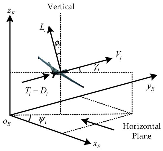
Figure 1.
Fixed-wing UAV model.
Considering a system composed of UAVs in 3D space, the mathematical model of the UAV is described as follows:
where is the index of the UAVs, and , , , and represent the position, speed, flight-path angle, and heading angle of the -th UAV, respectively. , , , and represent the mass, gravitational acceleration, lift, and drag, respectively. The actual control vector represents the thrust, g-load, and banking angle. Moreover, the constraints on the relevant variables are as follows: , , , , , and .
To facilitate the controller design, the component of along the coordinate axis is defined as , and the virtual control vector along the coordinate axis is defined as . The relationships between and are given as follows:
The flight-path angle and the heading angle are computed by and .
We denote the flight convex hull formed by the UAV swarm as , that is
Let
be the distance between the target and and
be the point in that has distance from the target, where represents the target’s position vector. It is obvious that if and only if . The target fencing diagram is shown in Figure 2.
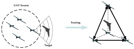
Figure 2.
Diagram of target fencing.
2.2. Dynamic Communication Topology
The interaction between UAVs can be described by graph , where is the set of nodes and is the set of edges. The weighted adjacency matrix of is denoted as . If the -th UAV can obtain the information from the -th UAV, ; otherwise, . We define the Laplacian matrix of as , where and .
Notice that the position distribution of the swarm is dynamically changing in accordance with the planned trajectory, and the UAV with sensing range is continually moving in 3D space. Therefore, the neighbor set of each UAV is constantly updated, resulting in a dynamic communication topology. We define the time-varying neighbor set of the -th UAV as follows:
where represents the Euclidean distance between the -th UAV and the -th UAV.
Remark 1.
In this paper, we assume that each UAV is equipped with the same onboard sensors and the -th UAV can be observed by the -th UAV if . Thus, graph is undirected and the Laplacian matrix is semi-positive definite.
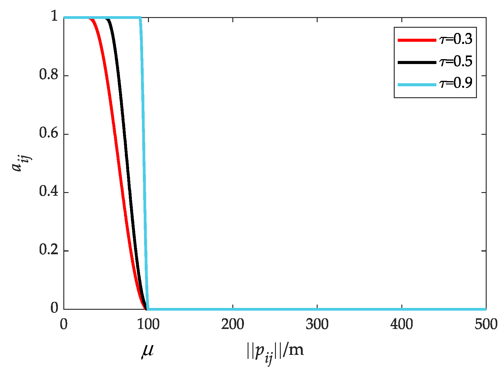
In practical applications, the performance of sensors is related to the distance between UAVs. Therefore, combined with the dynamic topology, the communication weight based on relative distance is defined as follows.
where is the communication decay rate. Figure 3 shows the evolution of the for different . It is obvious that smoothly varies from 1 to 0 by designing (7).
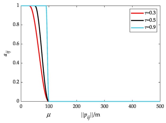
Figure 3.
Communication weights under different decay rates.
2.3. Control Objective
In specific mission scenarios, UAVs are required to cooperatively fence or capture high-value flying targets. To ensure the safety of the swarm, UAVs should possess autonomous collision and obstacle avoidance capabilities. Furthermore, the behaviors associated with collision or obstacle avoidance may lead to significant separation distances, resulting in losing connectivity between UAVs once . Hence, maintaining connectivity within the swarm holds crucial significance. Additionally, given the limitations of onboard sensors, the speed and control input of the target may not always be directly measurable, requiring the estimation of both. In the target fencing mission, our primary concern is the dynamic changes in the position and velocity of the UAV swarm relative to the target in 3D space. Consequently, in formulating the control law, we prioritize the virtual position and speed of the UAVs as the principal control variables. Combining the above analysis, the control objective can be expressed as follows.
(C1) The target’s speed and control input can be estimated within a fixed time, i.e., and , where represents target’s speed vector, and and represent the estimation of the target’s speed and control input for the -th UAV, respectively.
(C2) The target can be fenced by the UAV swarm, and each UAV’s speed converges to the target’s speed eventually, i.e., and .
(C3) Collision avoidance and connectivity maintenance: , where represents the body radius of the UAV.
(C4) Obstacle avoidance: , where represents the position vector of the obstacle, and represents the Euclidean distance between the UAV and the obstacle.
Remark 2.
(C2) means that there exists a flight trajectory , which enables the swarm to constantly fence the target, i.e., and the trajectory of the UAVs converges , where represents the Kronecker product [16].
3. Main Results
3.1. Differential State Observer
In the uncooperative scenarios, the UAVs and the target have a competitive relationship. Therefore, it is unreasonable for the UAVs to obtain and . Assuming that the target’s position can be measured by the UAVs through onboard sensors, we design a fixed-time state observer (8) to estimate and .
where represents the estimation of (i.e., , , and ) for the UAV. satisfies and belongs to for a sufficiently small . satisfies and belongs to for a sufficiently small . Observer gains and are selected such that the polynomials and are Hurwitz.
Theorem 1.
Based on the observer (8), and can be estimated within a fixed time
where and are the symmetric positive definite matrix. and satisfy the Lyapunov equation and , respectively, where and are Hurwitz.
Proof of Theorem 1.
We denote the observer error as and its derivatives take the form
Furthermore, (10) is rewritten as
Since and are Hurwitz, the systems and are asymptotically stable.
For the function , its time derivative yields
We define an energy function
where , , , and .
Based on [38], if , is the Lyapunov function for the error system (11). In view of (12), it implies that and
As noted in [38,39], the observer error converges to 0 within a fixed time, i.e., and . The convergence time is bounded by (9). Thus, (C1) is proved. □
Remark 3.
In [18], assuming a consistently connected communication topology, a network-based observer was designed to estimate the target’s state. In this paper, we address the challenge of maintaining connectivity within a dynamic topology and propose a differential state observer capable of simultaneously estimating the target’s velocity and control input, laying the foundation for UAV swarms to accurately fence a maneuvering target. Prior to commencing their tasks, the observer algorithm can be pre-integrated into the onboard computer, enabling real-time computation of speed and control input once the target’s position is acquired or detected.
3.2. Cooperative Fencing Controller
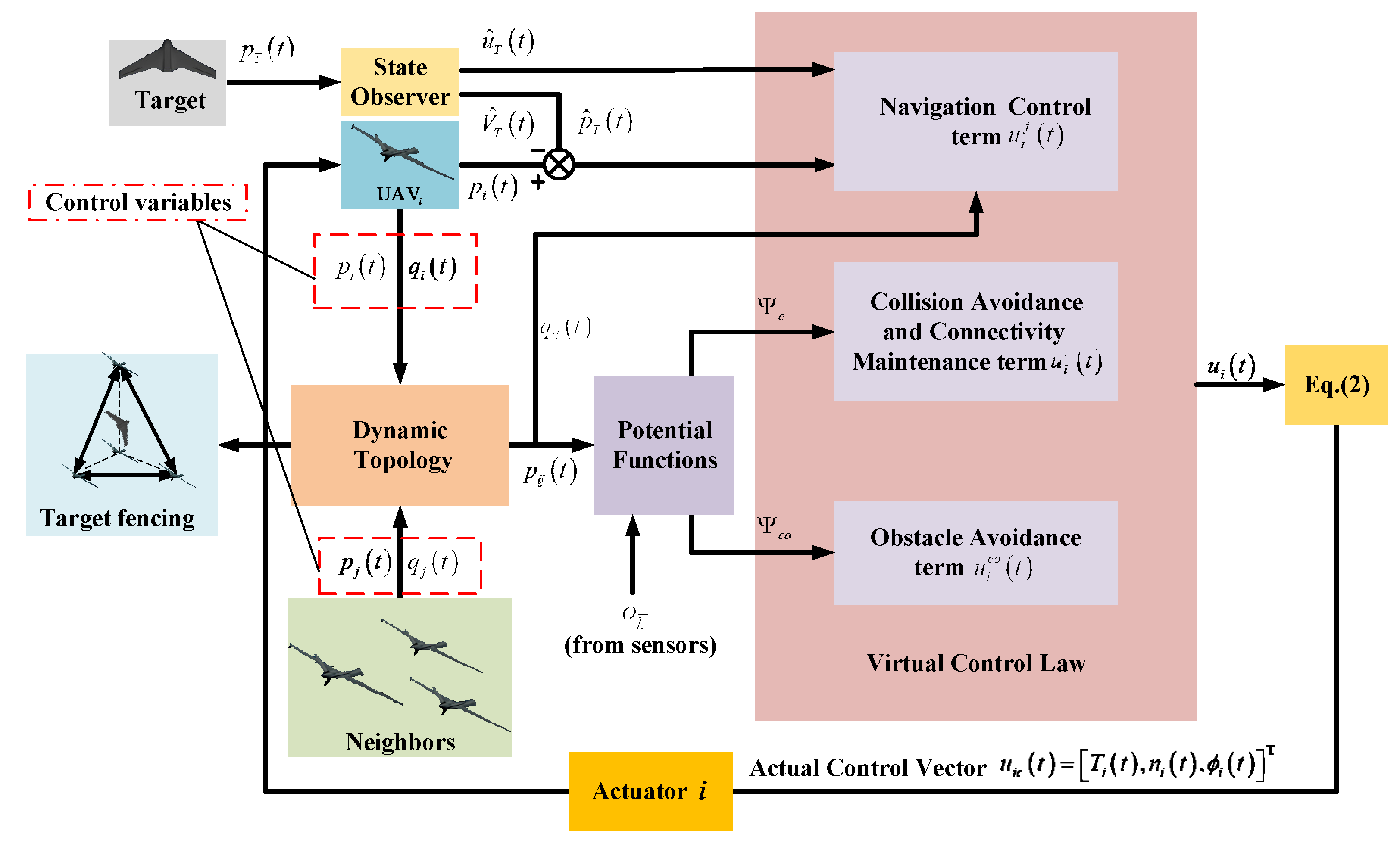
In this section, the cooperative target fencing controller designed for UAV swarms consists of three components: a navigation control term , a collision avoidance and connectivity maintenance term , and an obstacle avoidance term . The schematic diagram of the cooperative target fencing control is illustrated in Figure 4.
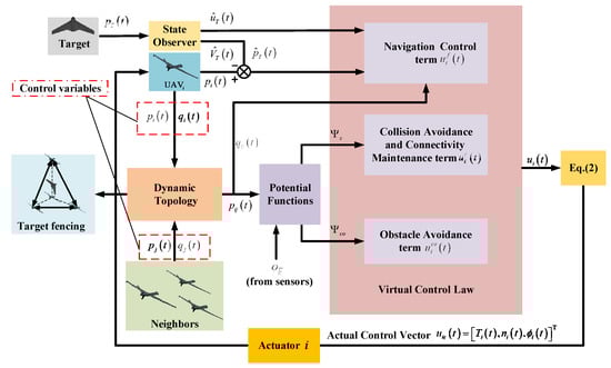
Figure 4.
Schematic diagram of the UAV swarm cooperative target fencing control.
3.2.1. Navigation Control Term
Given that the primary objective of the UAV swarm is to fence the target, it is imperative to guide each UAV towards the target using the navigation control term. Moreover, each UAV must maintain a consistent flight speed that aligns with the target’s speed to preserve a stable convex hull and ensure continuous target fencing. To fulfill these requirements, is designed, as follows:
where the control gains and are positive constants.
Remark 4.
In (15), introduces a feedback term about the relative distance between the UAV and the target, serving solely as an attractive term to drive the UAVs towards the target, rather than directing them to converge to the target’s position. The collision avoidance term in Section 3.2.2 ensures that the relative distance between each UAV is automatically maintained, thus guaranteeing the existence of the convex hull and enabling the swarm to fence the target.
3.2.2. Collision Avoidance and Connectivity Maintenance Term
To facilitate real-time collision avoidance, we propose a modified potential field method that incorporates the physical radius of each UAV into the design of the potential function, in contrast to previous studies [21,22,23,24,25], where the agent was treated as a particle.
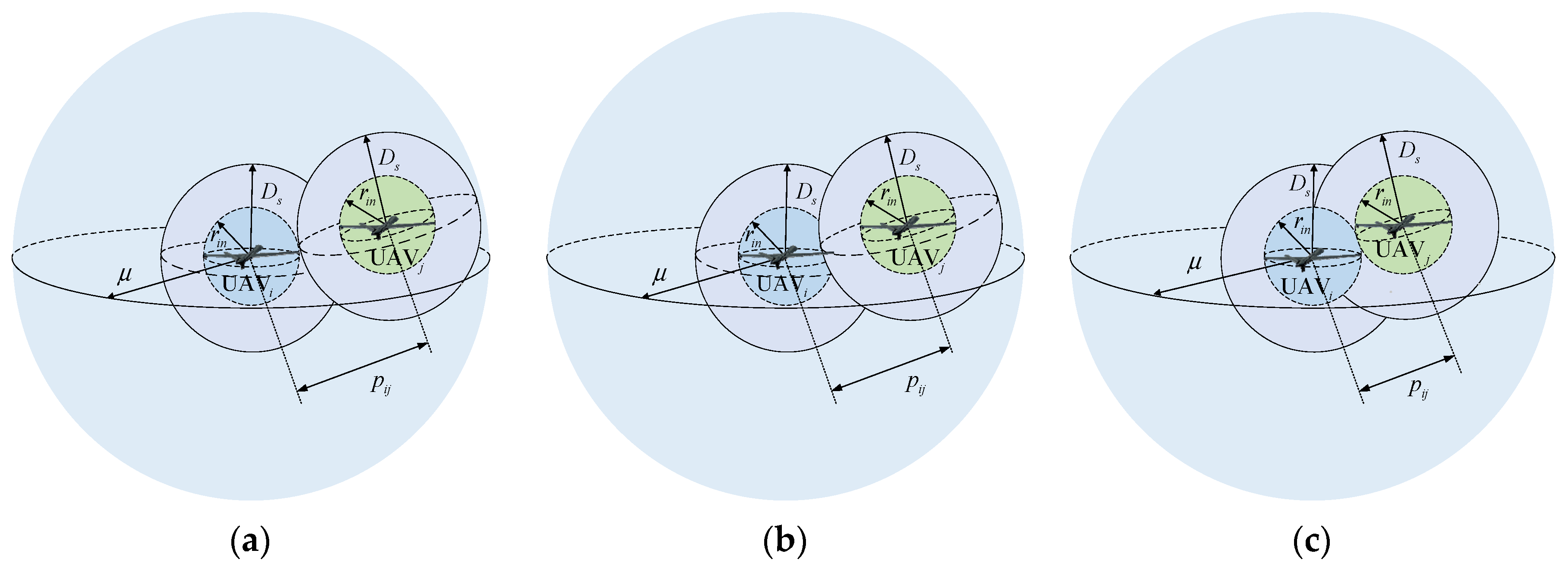
Assume that the collision avoidance radius of each UAV is . To ensure collision avoidance and connectivity maintenance among UAVs, each UAV should be encompassed by both attractive and repulsive potential fields. As described in Figure 5a, when the relative distance between UAVs, they are positioned at a safe distance and the repulsive force remains . In Figure 5b, as they continue to approach, that is, , the UAV triggers the repulsive potential field of the UAV, resulting in the repulsion between them. In Figure 5c, represents the minimum safe distance between them and the corresponding repulsive force .
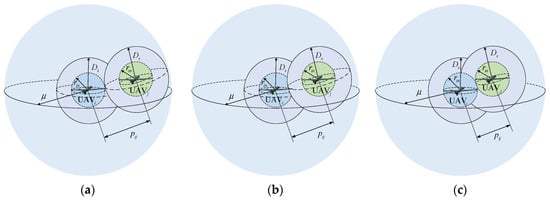
Figure 5.
Schematic diagram of collision avoidance and connectivity maintenance potential field. (a) ; (b) ; (c) .
Moreover, due to the movement of the UAV and the repulsive force, it is possible for the UAV to be positioned outside of the sensing range, that is, , resulting in a loss of connectivity between them. To address this problem, we construct an attractive potential field and constrain their relative distance within .
In summary, the UAV and the UAV exhibit repulsive behavior when , while exhibiting attractive behavior when . Based on the above analysis, the potential function including collision avoidance and connectivity maintenance is defined as follows:
Remark 5.
Given that collision avoidance and connectivity maintenance rely on the constraint of relative distance between UAVs, we draw inspiration from [40] to design a potential field function for achieving these two functionalities. Although target fencing control with a collision avoidance strategy has been investigated in [16,17,18], these studies generally assume that the topology between UAVs is consistently connected with time-invariant communication weights. However, in practical scenarios, it is difficult to meet these idealized conditions.
Considering the neighbor set and the time-variant communication weights, the potential-based control term is formulated as
where is the control gain and represents the gradient of along .
3.2.3. Obstacle Avoidance Term
Assumption 1.
The flight trajectory of the target is ideal under , that is, no problems of obstacle avoidance arise with the target.
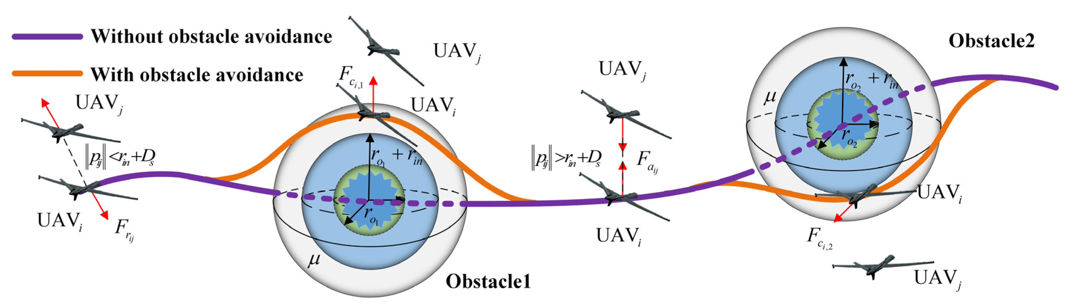
The obstacle avoidance potential field is defined similarly to Section 3.2.2, with the exception that the attractive term is omitted. Consider that an obstacle is surrounded by a sphere with a radius of , and set the safe obstacle avoidance distance as , where represents the obstacle avoidance margin parameter. When the UAV detects the obstacle within its sensing range , it actively maneuvers away from the obstacle under the repulsive force .
To further illustrate the obstacle avoidance process of the swarm, a schematic diagram of the obstacle avoidance potential field is shown in Figure 6. It is noteworthy that this paper distinguishes itself from others solely focused on obstacle avoidance by also considering collision avoidance and connectivity maintenance among UAVs within the context of obstacle avoidance.

Figure 6.
Schematic diagram of obstacle avoidance process.
The obstacle avoidance potential function can be designed as follows:
Then, the control term is
where is the control gain, is designed later, and represents the gradient of along .
Remark 6.
In (19), UAVs have the capability to obtain obstacle positions, with obstacle detection being performed through airborne sensing equipment. For instance, the UAV utilizes visual and laser sensors to perceive the flight environment and measure the relative distance to obstacles, thereby calculating control commands required to avoid obstacles.
Combined with the above analysis, we have developed a cooperative fencing controller (22) for UAV swarms:
Remark 7.
This paper adopts the method of the segmented design of potential fields to address collision, obstacle avoidance, and connectivity maintenance problems simultaneously. Compared to the traditional APF methods, the potential functions in this paper exhibit smooth variability, which avoids the saltation phenomenon of the controller. When obstacle avoidance and connectivity maintenance are not considered, the controller (19) can also be effectively applied to solve the target fencing control problem in [18].
3.3. Stability Analysis
Assumption 2.
The initial state of the UAV is chosen to satisfy , , and .
Theorem 2.
Supposing that Assumptions 1–2 hold and the control parameters satisfy the aforementioned requirements, the fixed-wing UAV swarm is capable of effectively fencing a maneuvering target under the control law (22). Moreover, the control law facilitates collision, obstacle avoidance, and connectivity maintenance throughout the target fencing process.
Proof of Theorem 2.
According to Theorem 1, the target’s speed and control input can be observed by UAVs within a fixed time, i.e., and . Thus, the controller (22) can be transformed into
The control objectives (C2)–(C4) will be proved in four steps. The first part is to prove the system stability without obstacles.
Step 1: Proof of target fencing stability
For convenience, we denote as the position error between the UAV and the target, as the average position error, as the speed error between the UAV and the target, and as the average speed error.
The time derivative of yields
Then, differentiating ,
Based on the definition of a dynamic network in Section 2.2, which states that the communication between UAVs is undirected, it is implied that and . We have and .
Thus, (25) can be transformed into the following system
Due to , it is obvious that (26) is stable. and exponentially converge to zero as . It implies that and , i.e., the target is fenced by the swarm.
Step 2: Proof of convergence for UAVs’ speed
We denote the following Lyapunov function candidate as
The time derivative of (27) is
where . Since the Laplacian matrix is positive semi-definite, is positive definite, and , it follows that matrix is positive definite. Hence, indicates . Combined with Theorem 1 in [40], it can be shown that is an invariant set and all solutions starting from for Equation (29) will converge to the largest invariant set .
Therefore, , i.e., , which means that the speeds of each UAV can consistently converge to the target’s speed. With this, the control objective (C2) is proved.
Step 3: Proof of collision avoidance and connectivity maintenance
To prove (C3), the Lyapunov function is constructed as follows
where vectors , , and .
Taking the derivatives of gives
Substituting (23) into (31), we have
In view of (30) and (32), it is derived that
If , then , which contradicts Equation (33). Hence, , that is, collision avoidance can be achieved between UAVs.
Note that, according to the potential field function defined in (16), if , UAVs are affected by repulsive force, leading to an increase in the inter-UAV distance. As the distance extends to , UAVs are impacted by the attractive force, leading to a decrease in the inter-UAV distance. By appropriately designing the potential field gain , the connectivity within the swarm is maintained. The control objective (C3) is proved.
Step 4: Proof of obstacle avoidance
We choose a Lyapunov function candidate as
Differentiating with respect to time, we have
Given that the dwell time of the UAV in is finite, the terms in (35) are bounded except . From the definition of the obstacle avoidance potential field function, if , then . As the UAV approaches the obstacle, we can derive the following inequality.
Substituting (23) into (31), we have . And the following inequality
holds, where is bounded in . Hence, we design the parameter appropriately such that . As a consequence, no collision occurs between UAVs and obstacles throughout the target fencing process.
It is worth noting that through Steps 1–3, we have demonstrated the stability of the system outside of . Therefore, we do not need to prove the stability of the system during the obstacle avoidance process, and it is only necessary to illustrate that under the action of the obstacle avoidance potential function, each UAV can avoid collision with obstacles. The control objective (C4) is proved.
In summary, the target fencing with collision, obstacle avoidance, and connectivity maintenance is achieved. The proof of Theorem 2 is completed. □
4. Numerical Simulation
In this section, we conduct two simulations to verify the effectiveness of the cooperative target fencing control strategy by the MATLAB R2020a platform. In the first scenario, the cooperative fencing of a target moving with a constant speed in a UAV swarm in an obstacle-free flight environment is validated. In the second scenario, it verifies that the same UAV swarm can fence a maneuvering target cooperatively in the presence of obstacles.
The parameters of the UAV model are selected from [37]. and are calculated by (38).
where , , and represent the atmospheric density, the wing area, and the zero-lift drag coefficient, respectively. The rest of the parameters in the model are the include coefficient , the load-factor effectiveness , and the weight of the UAV . The constraints on the actual control variables are , , and . Moreover, the body radius of each UAV is set to and sensing range is .
4.1. Scenario 1: Fencing a Target with a Constant Speed without Obstacles
Consider fencing the target with four UAVs. The initial speed of the UAV is randomly chosen from . The controller parameters are selected as follows: , , and . The communication decay rate is set as . The parameters of the potential field are , , and .
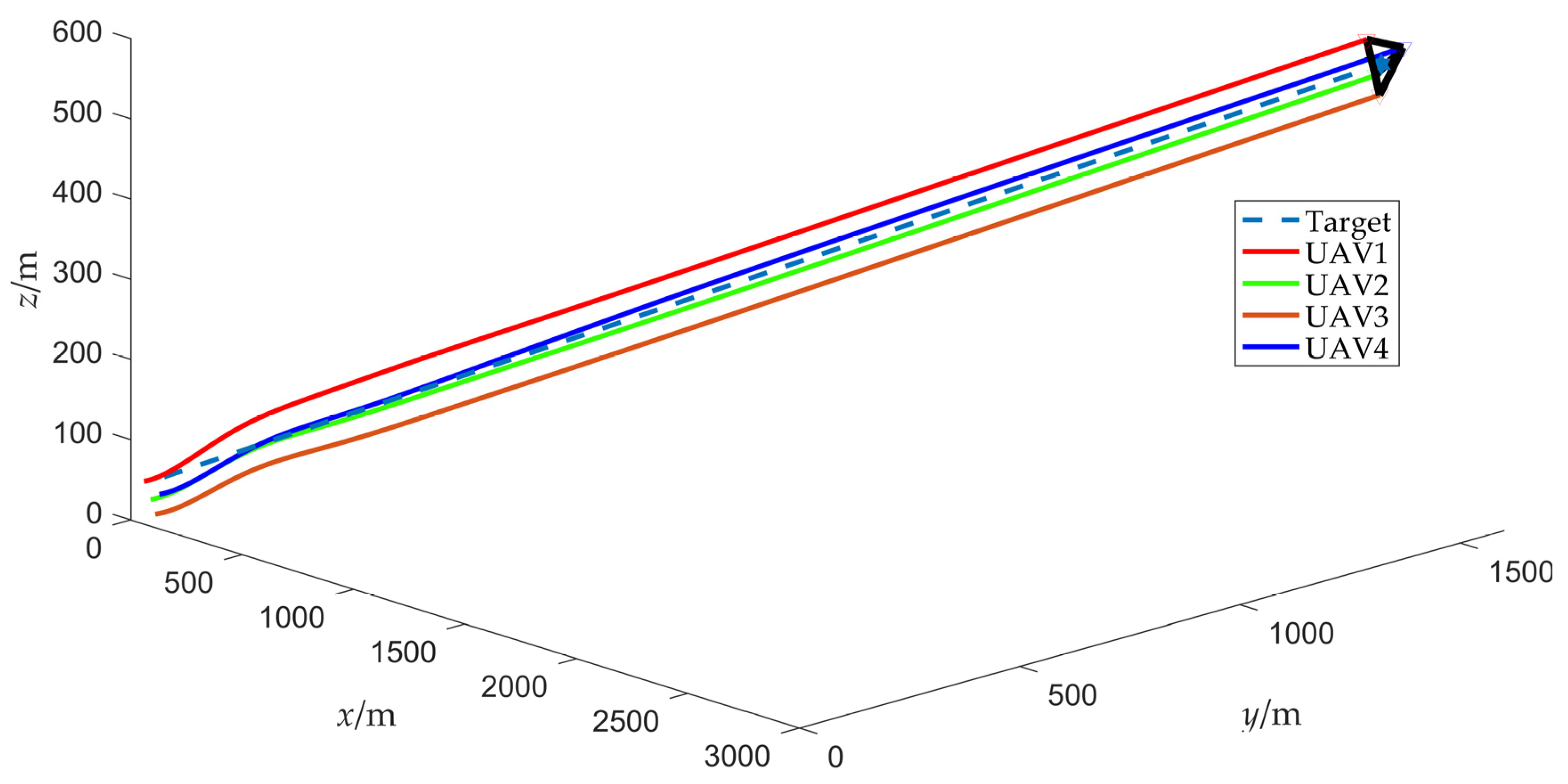
The simulation results of scenario 1 are shown in Figure 7, Figure 8, Figure 9, Figure 10, Figure 11, Figure 12, Figure 13, Figure 14 and Figure 15. Among them, Figure 7 and Figure 8 plot the target fencing trajectories and the final state of the UAV swarm under the controller (22), where the hexagram and triangle represent the target and the UAVs, respectively.
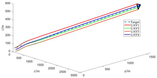
Figure 7.
Trajectories of UAV swarm during target fencing control (without obstacles).
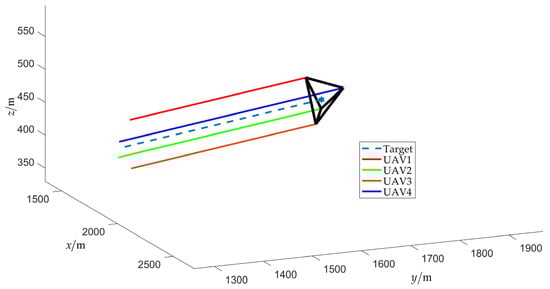
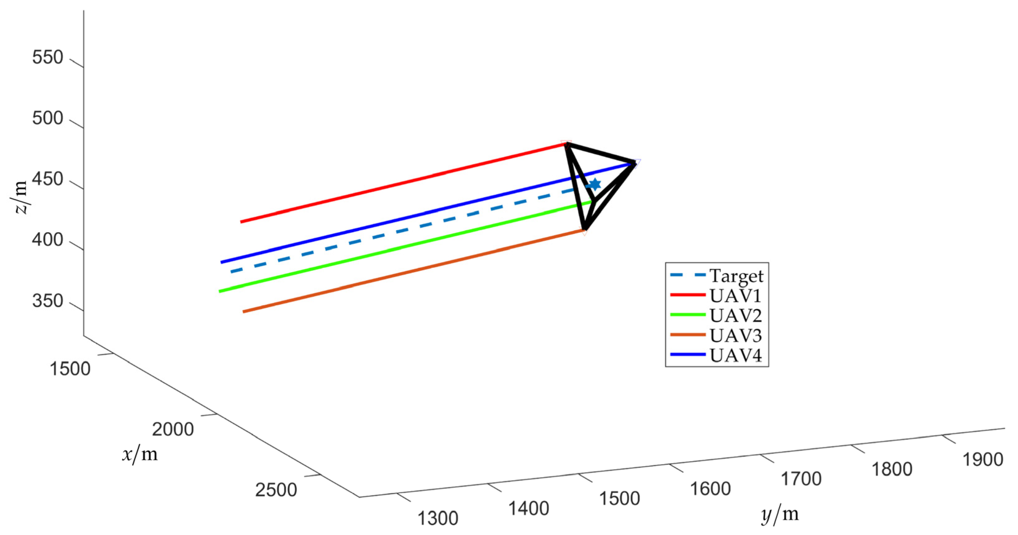
Figure 8.
Final fencing state (without obstacles).
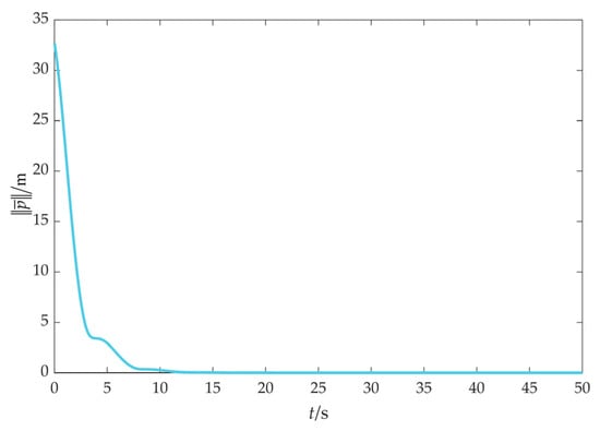
Figure 9.
Cooperative fencing error (without obstacles).
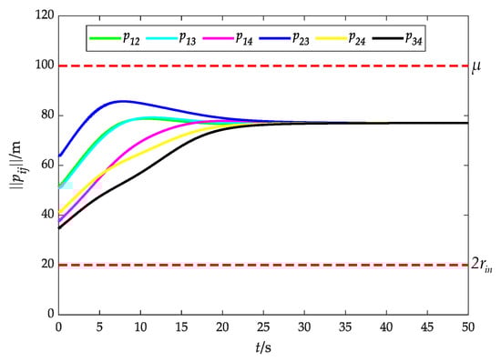
Figure 10.
Relative distance between UAVs without obstacles.
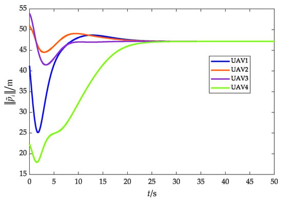
Figure 11.
Relative distance between UAVs and the target (without obstacles).
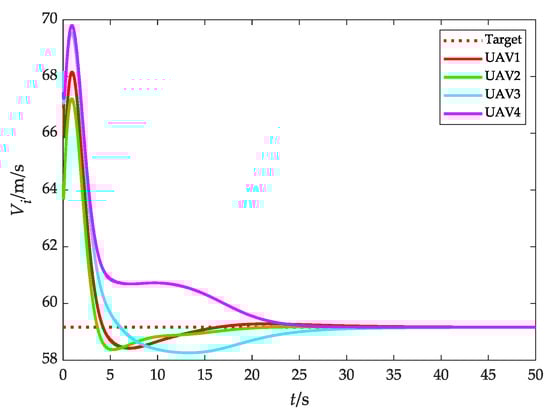
Figure 12.
Flight speed (without obstacles).
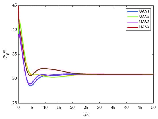
Figure 13.
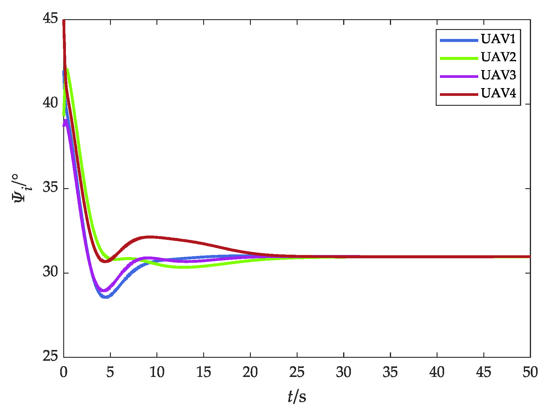
Heading angle (without obstacles).
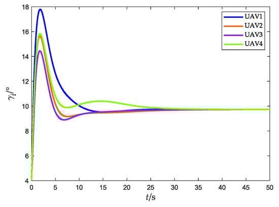
Figure 14.
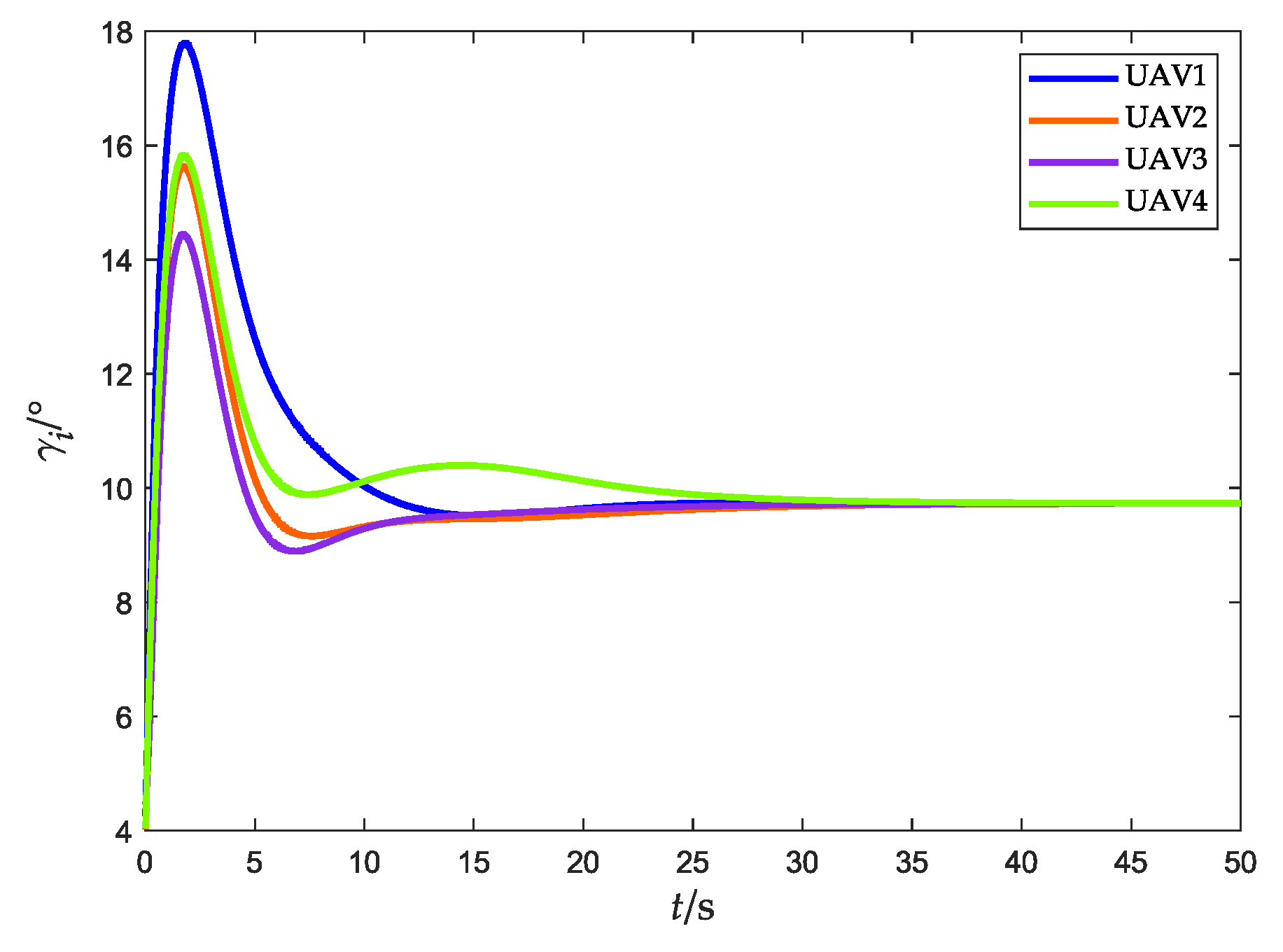
Flight-path angle (without obstacles).
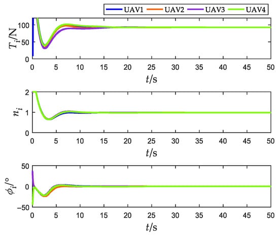
Figure 15.
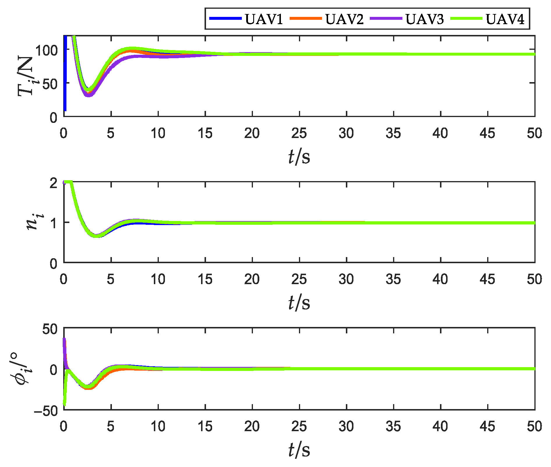
Actual control variables (without obstacles).
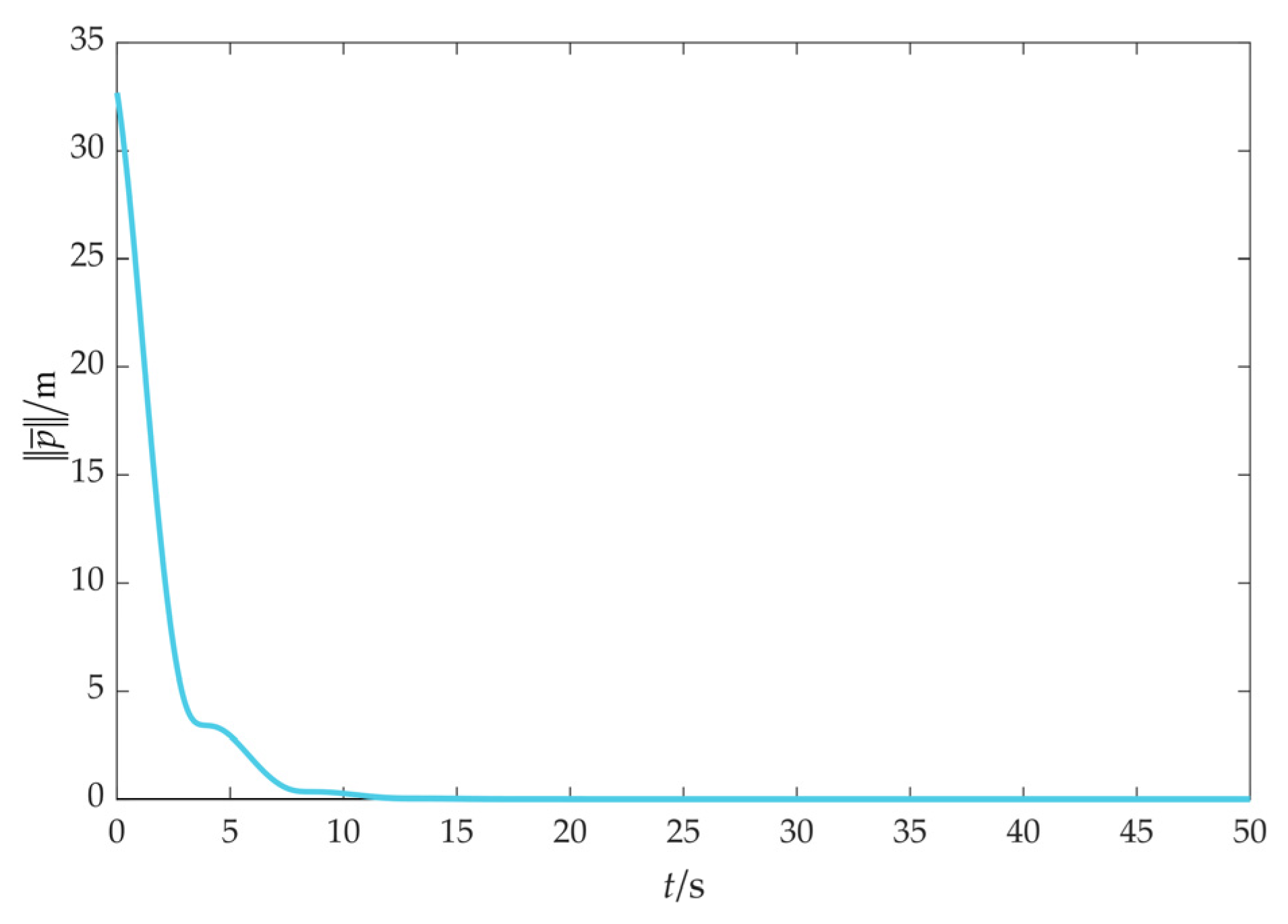
As depicted in Figure 9, the fencing error converges to 0, which means that the UAV swarm can fence the target, indicating that the effectiveness of the cooperative fencing strategy based on the flight convex hull is demonstrated.
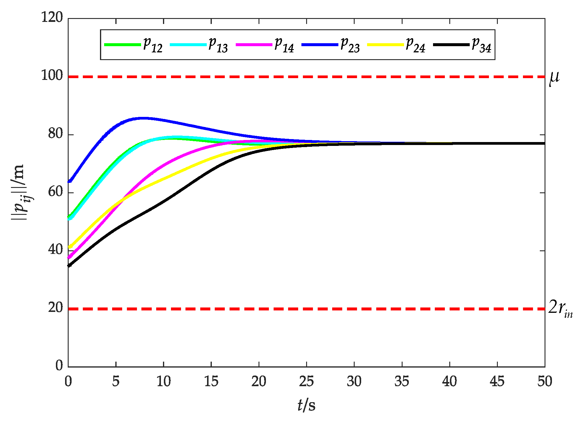
Figure 10 illustrates the relative distance between UAVs, and it is obvious that is consistently upheld during the fencing process, that is, UAVs can avoid collision and maintain the connectivity under the potential function (16).
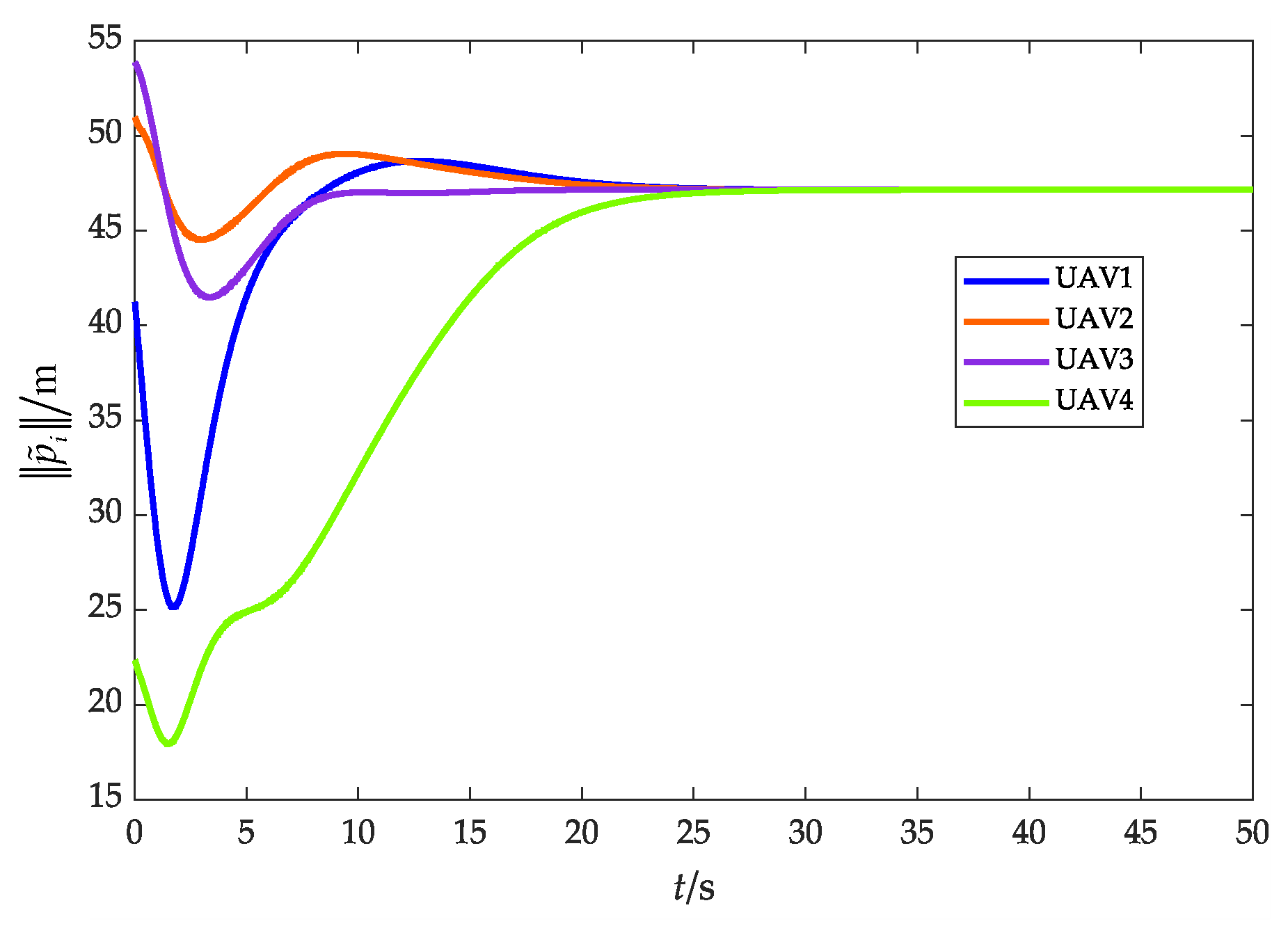
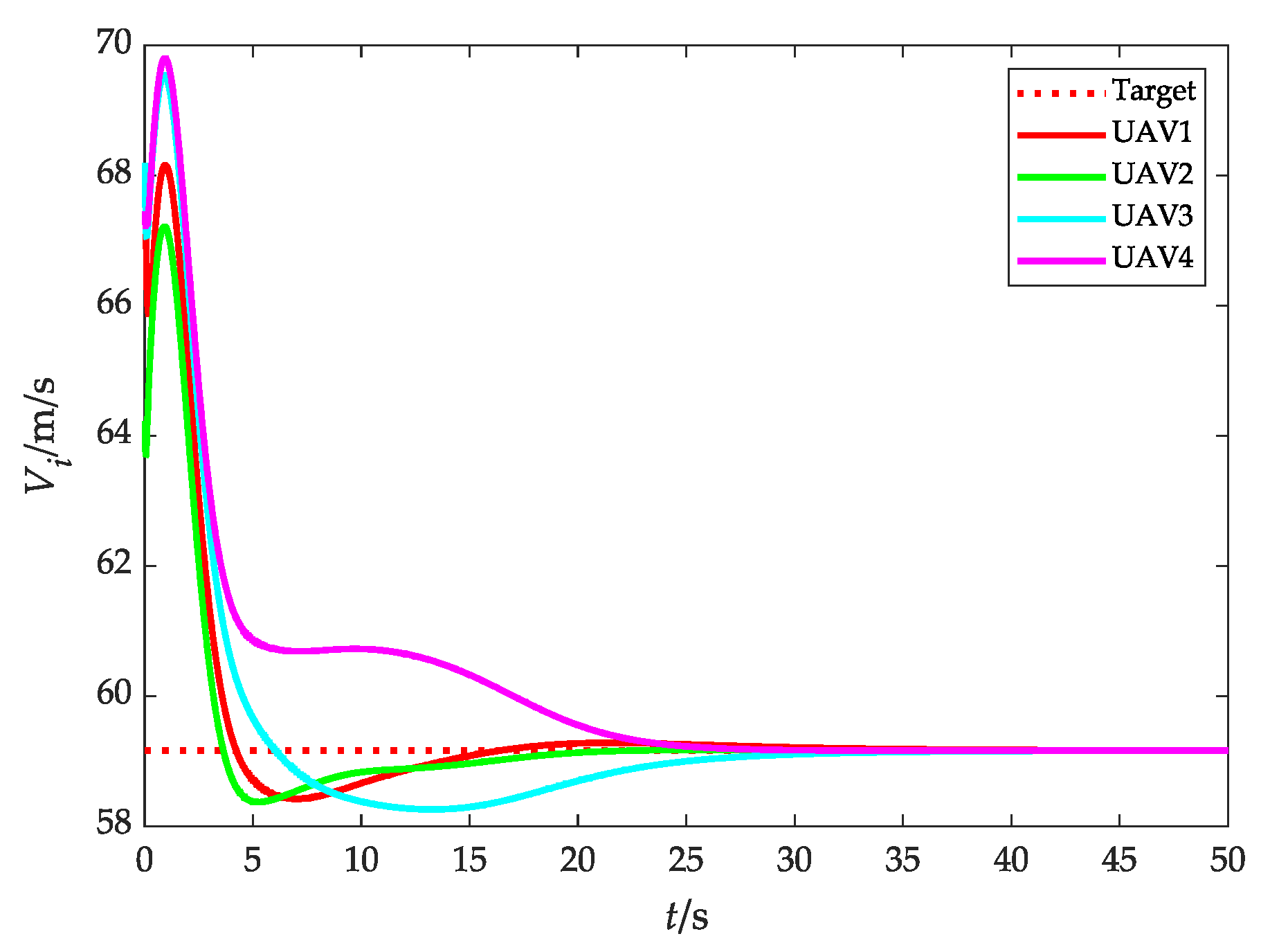
Figure 11 and Figure 12 show the relative distance and flight speed, and each UAV maintains a fixed distance from the target while moving at a consistent speed. Combined with Figure 10, it can be seen that the UAV swarm is capable of achieving a stable flight convex hull configuration and fence the target, which further explains Remark 4 in Section 3.2.1.
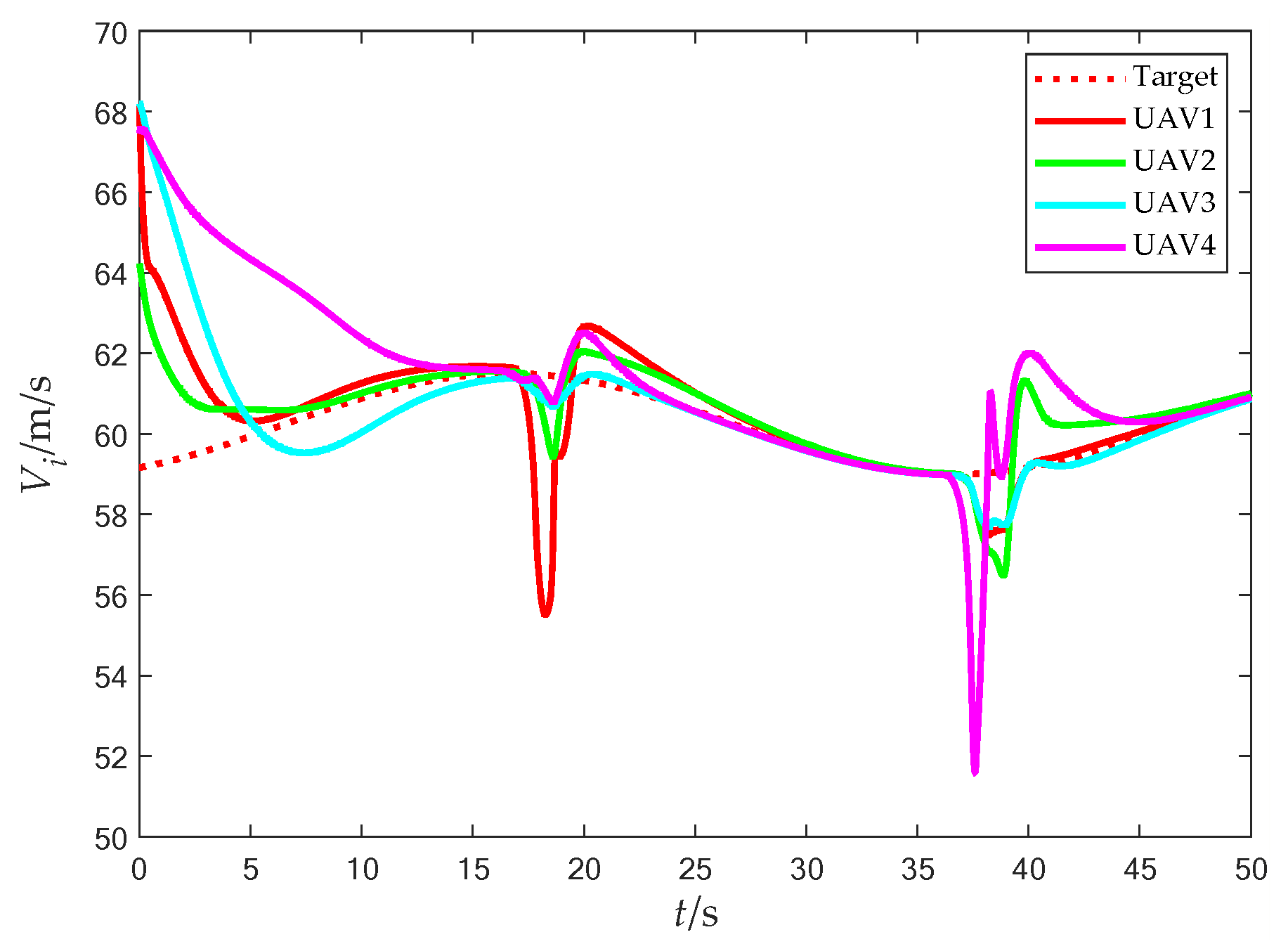
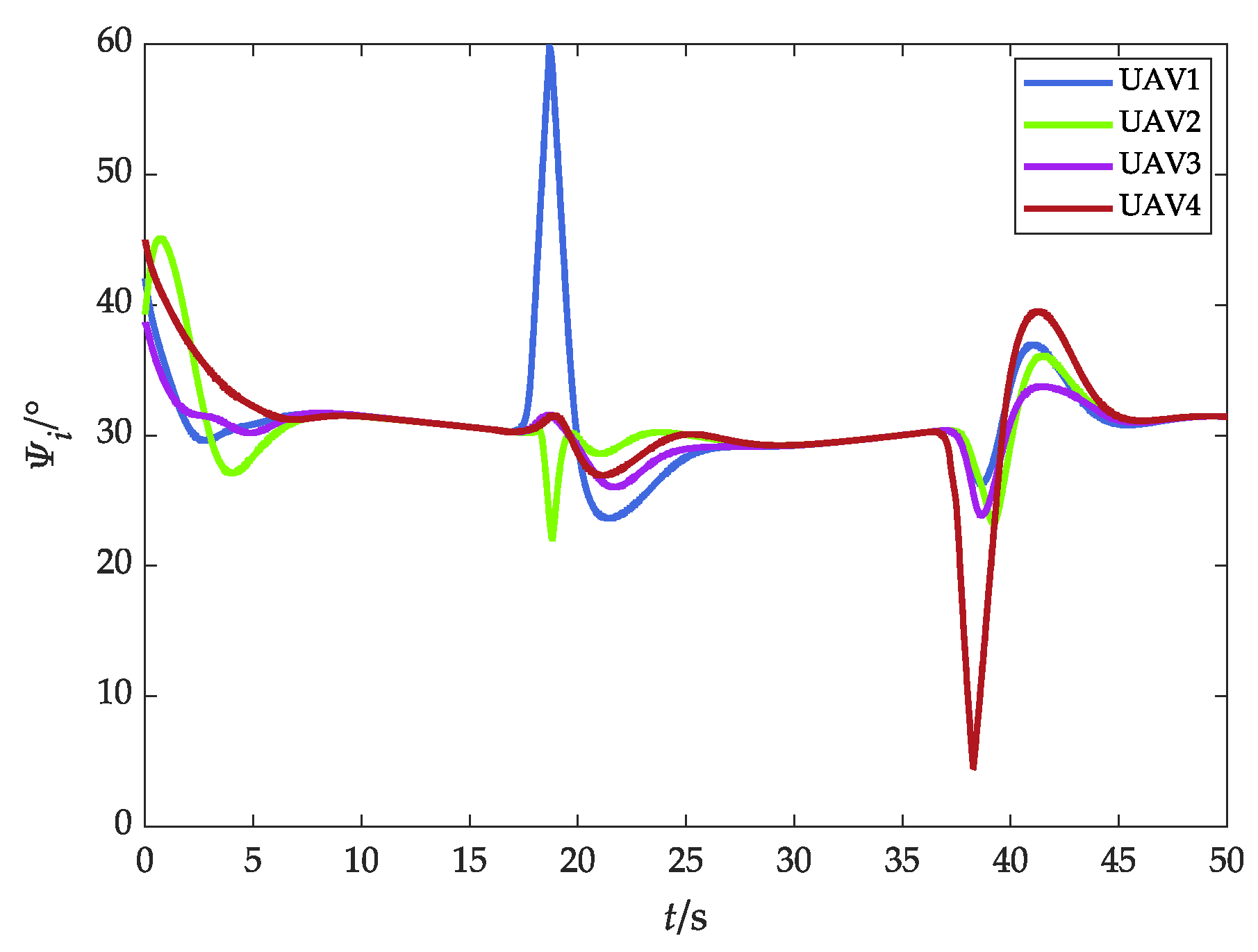
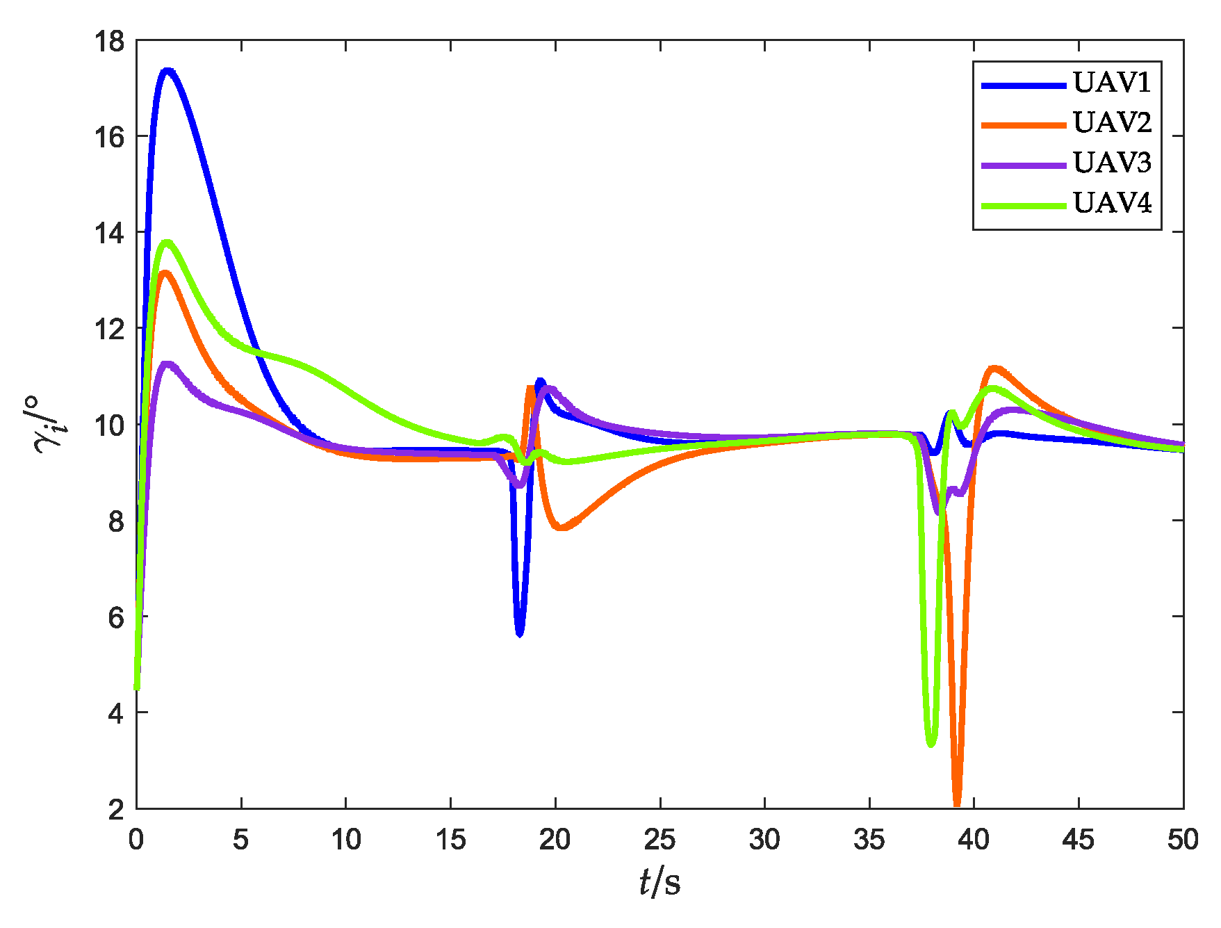
4.2. Scenario 2: Fencing a Maneuvering Target with Obstacle Avoidance
This section mainly demonstrates the effectiveness of the control law for fencing a maneuvering target considering obstacle avoidance. The target’s control input is set as , which is unknown to the UAVs. The controller parameters are , , and . Other parameters are the same as those in Section 4.1.
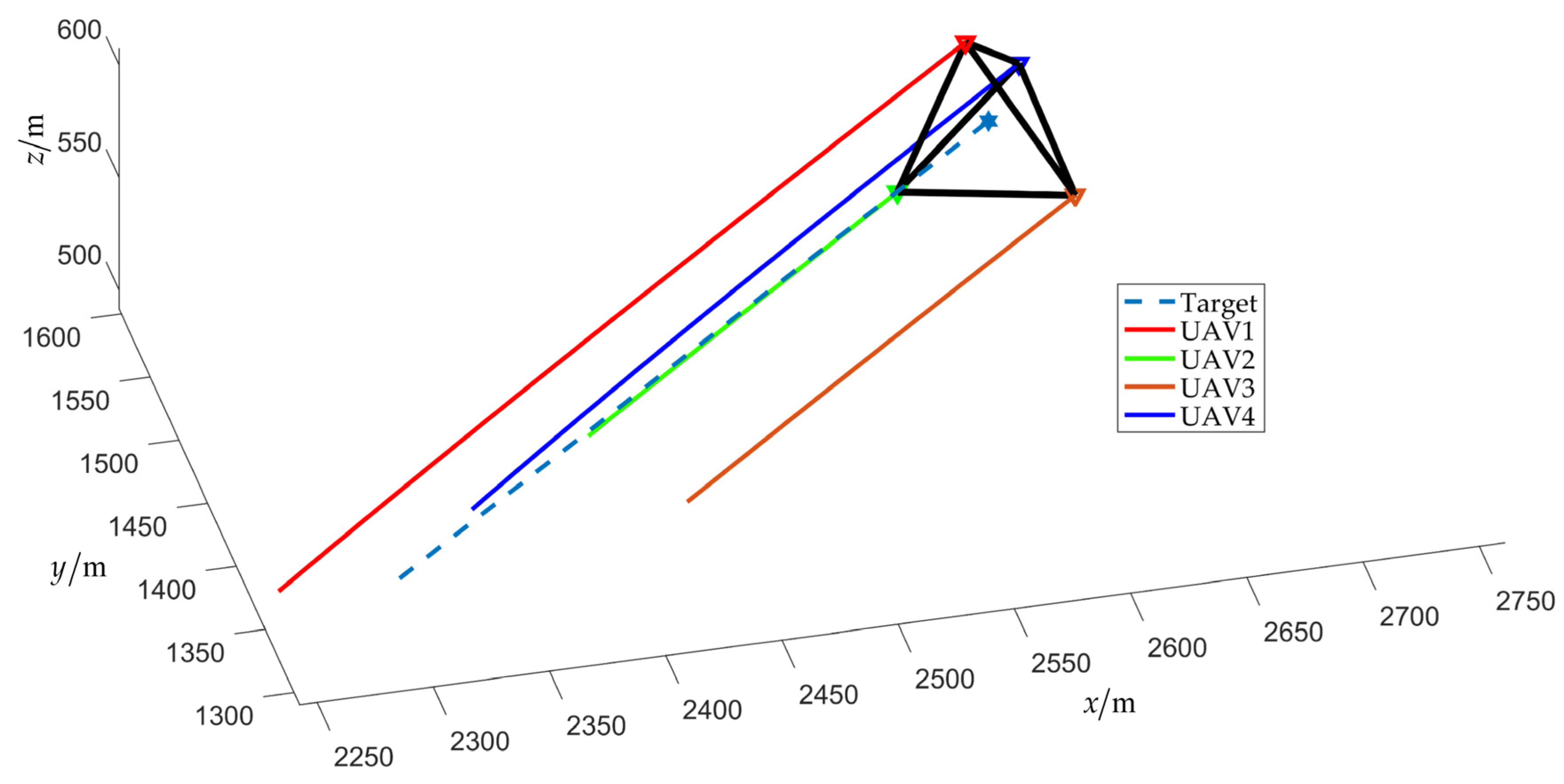
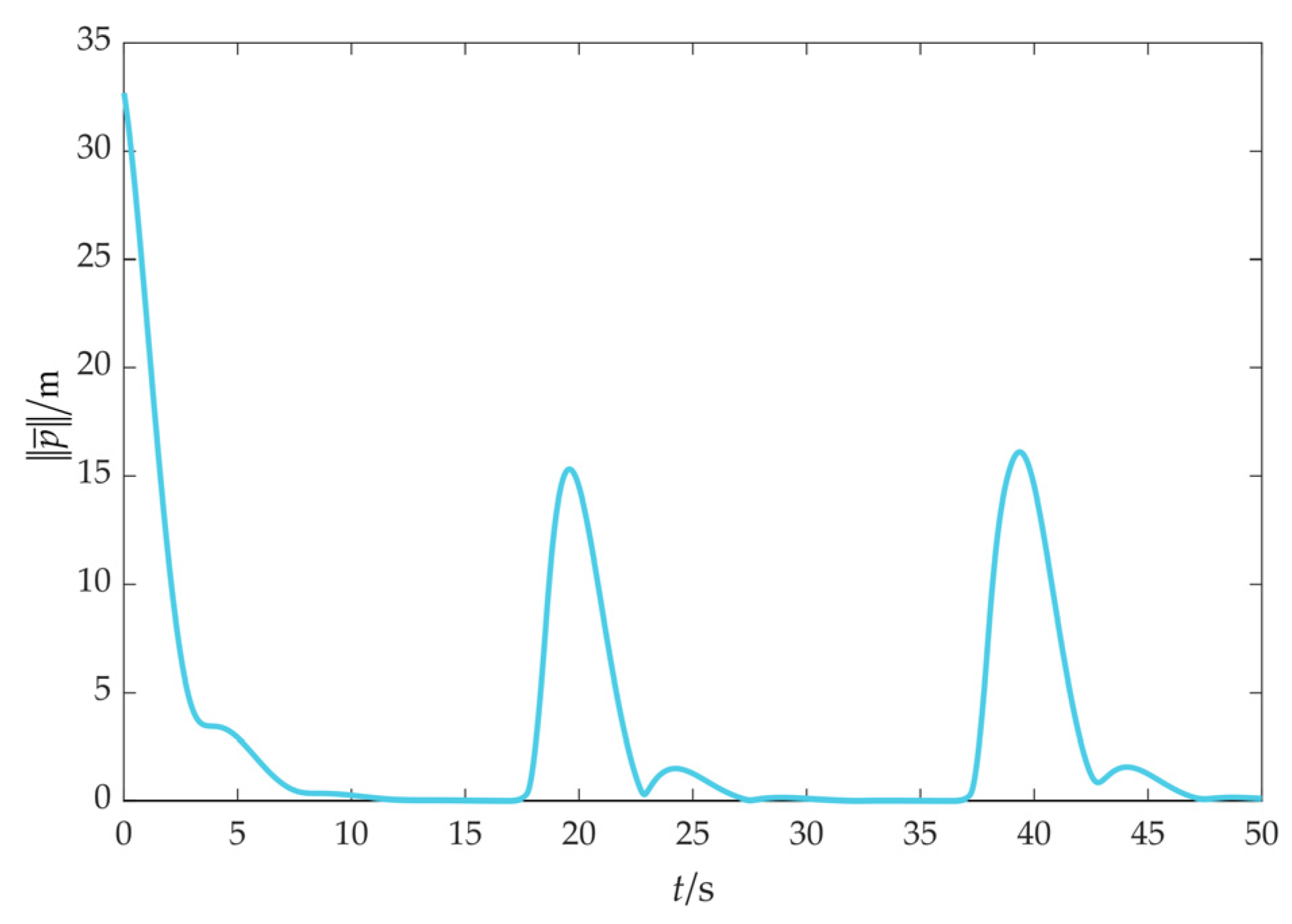
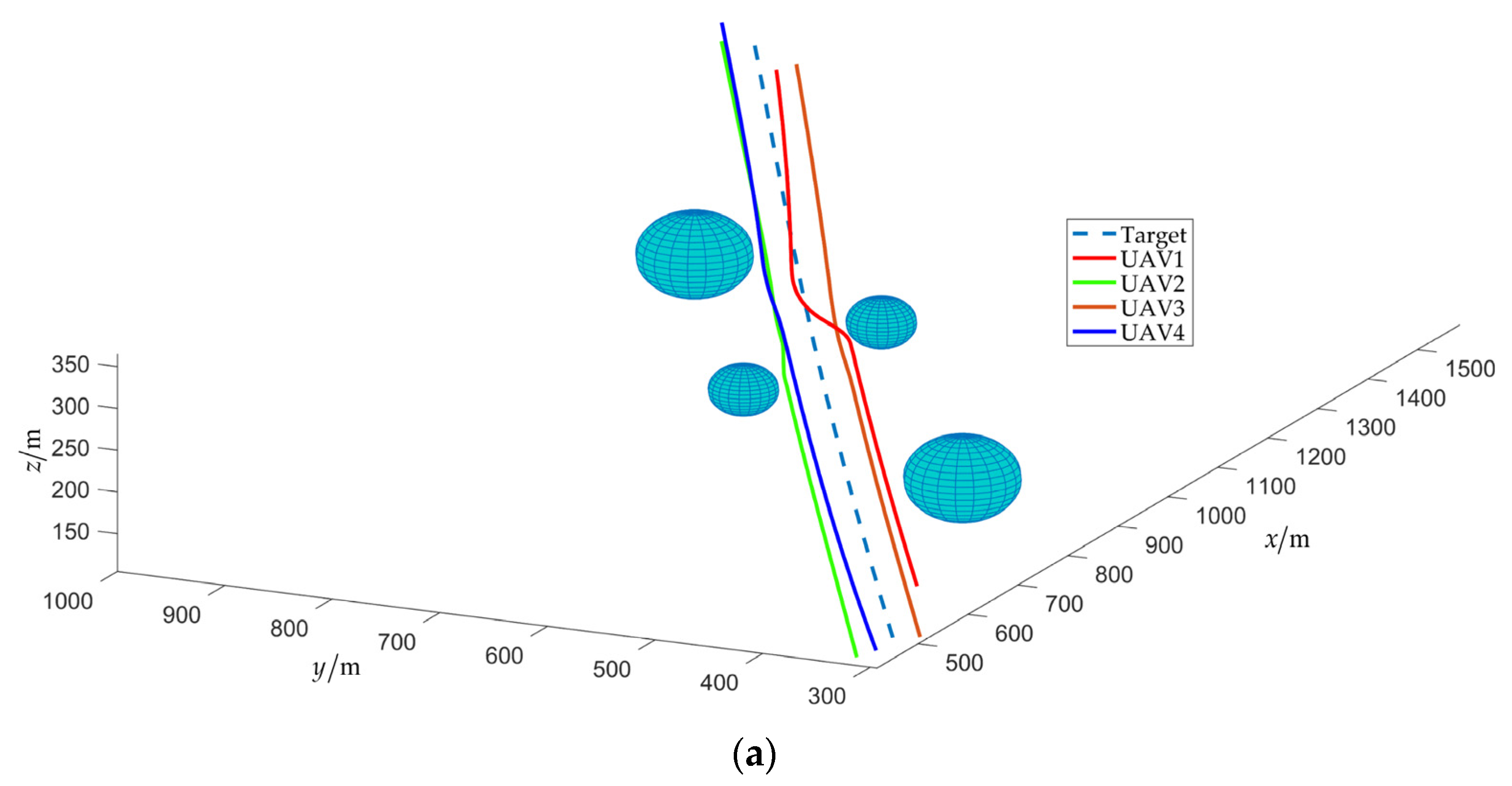
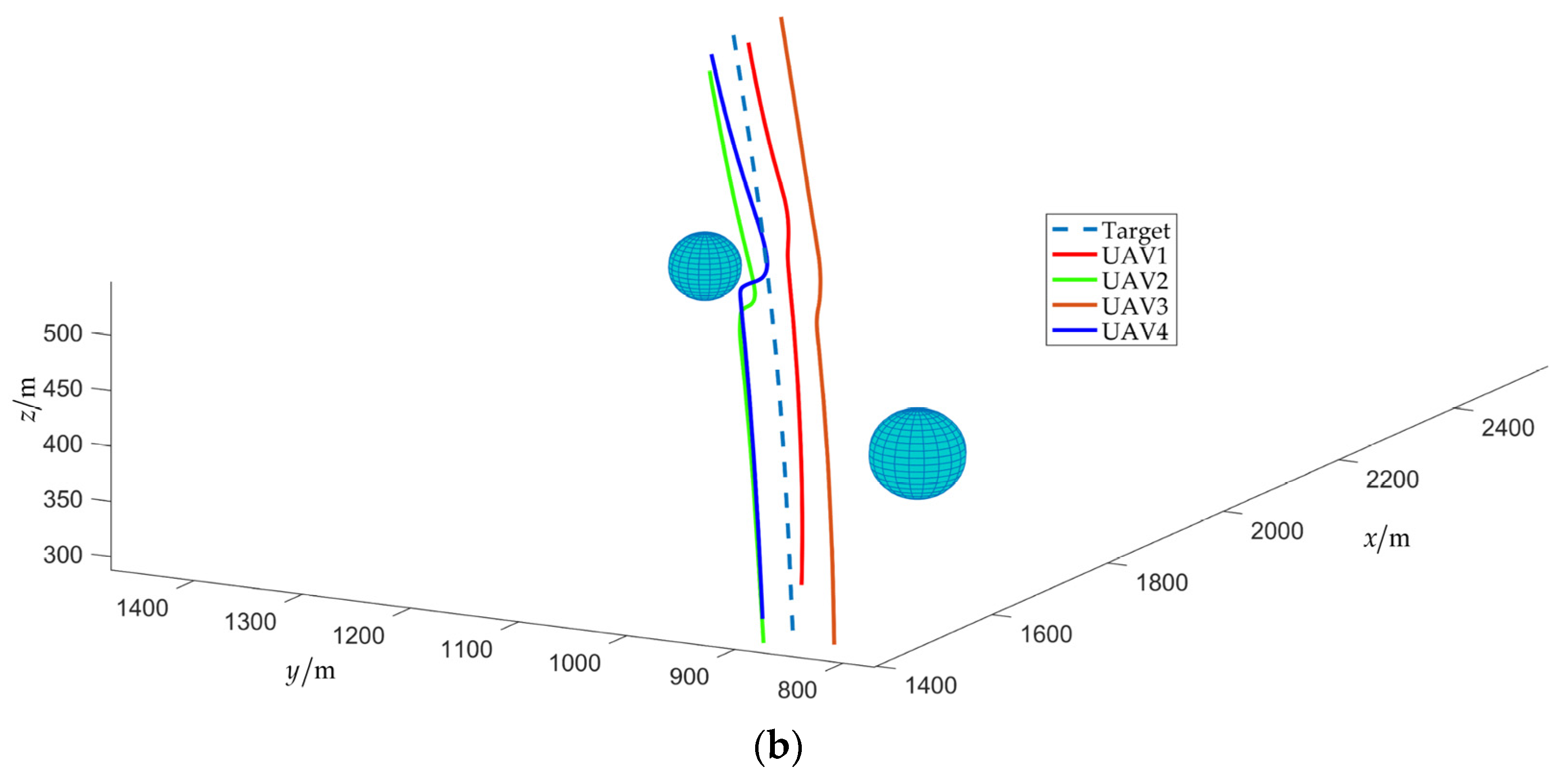
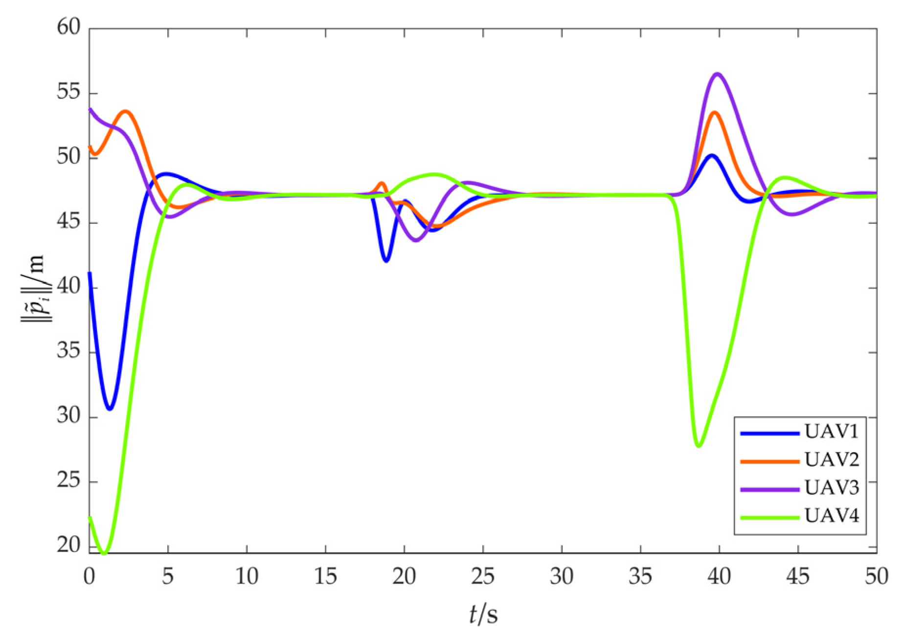
The simulation results of scenario 2 are shown in Figure 16, Figure 17, Figure 18, Figure 19, Figure 20, Figure 21, Figure 22, Figure 23, Figure 24 and Figure 25. Among them, Figure 16, Figure 17 and Figure 18 demonstrate that a maneuvering target remains to be fenced by the UAV swarm within an obstacle environment. Despite that the cooperative fencing error temporarily increases during obstacle avoidance, it can still rapidly converge to 0.
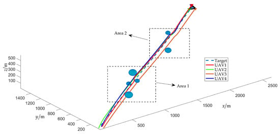
Figure 16.
Trajectories of the UAV swarm during target fencing control (with obstacles).
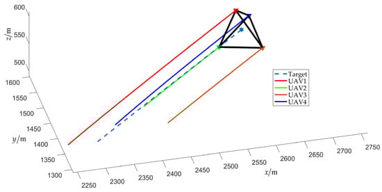
Figure 17.
Final fencing state (with obstacles).
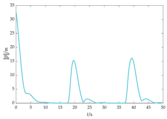
Figure 18.
Cooperative fencing error (with obstacles).
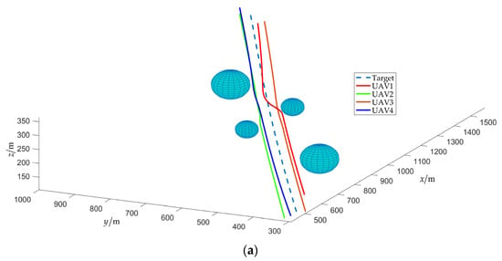
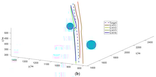
Figure 19.
Schematic diagram of obstacle avoidance. (a) Area 1; (b) area 2.
Figure 20.
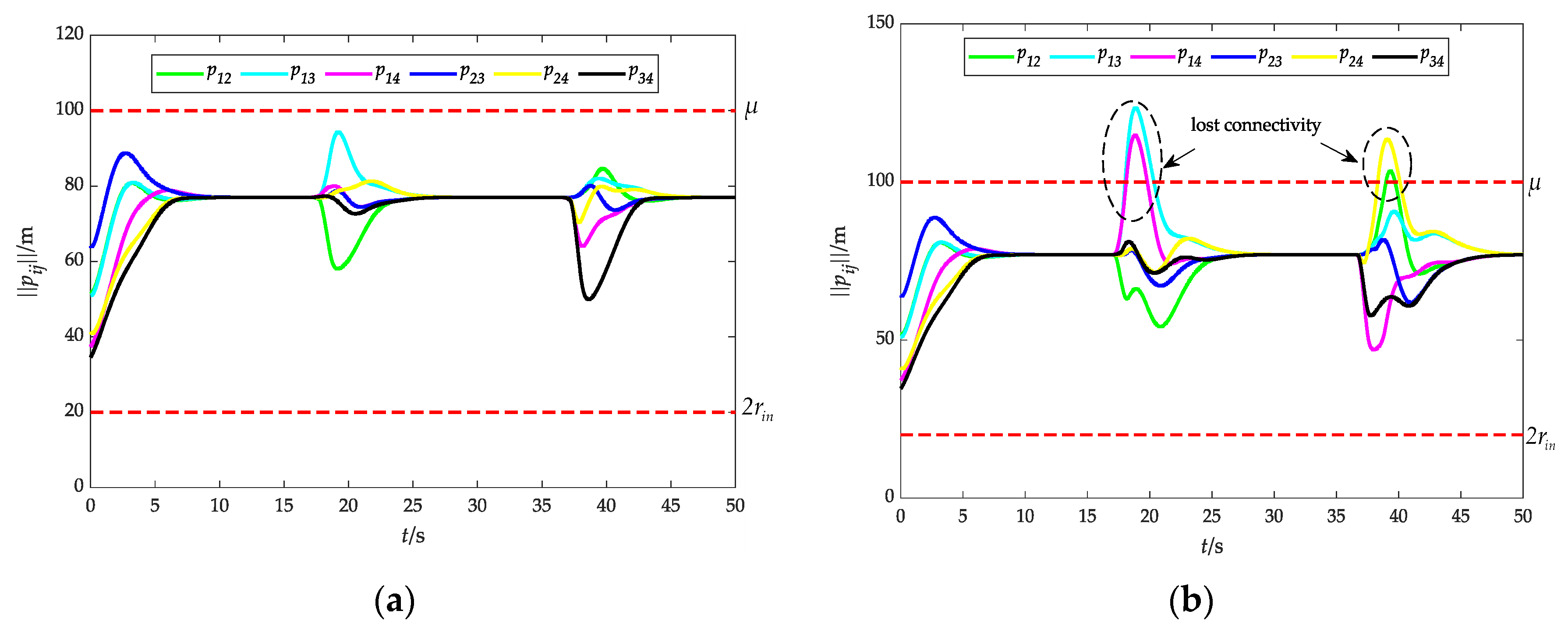
Relative distance between UAVs (with obstacles) (a) with connectivity maintenance; (b) without connectivity maintenance.
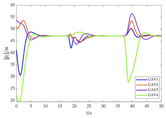
Figure 21.
Relative distance between UAVs and the target (with obstacles).
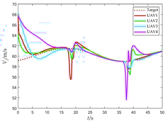
Figure 22.
Flight speed (with obstacles).
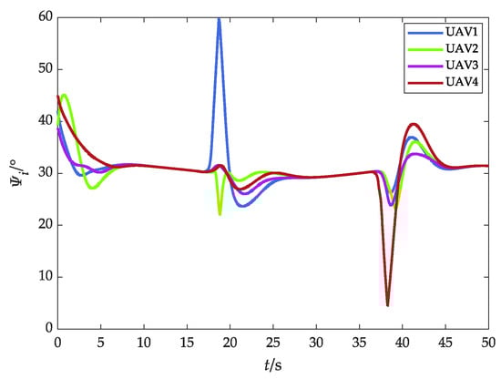
Figure 23.
Heading angle (with obstacles).
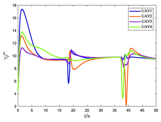
Figure 24.
Flight-path angle (with obstacles).
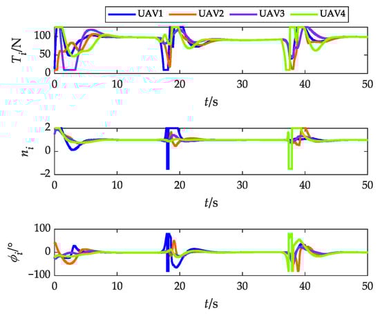
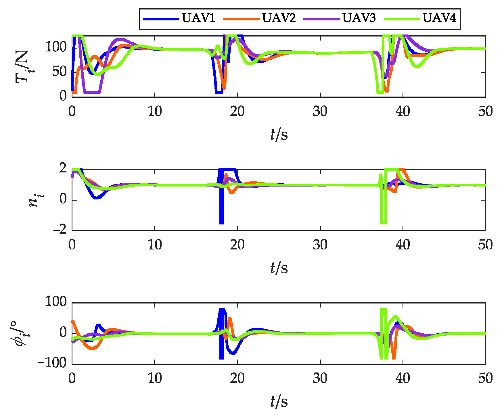
Figure 25.
Actual control variables (with obstacles).
Figure 19 shows a partial schematic of the obstacle avoidance process, and it is obvious that is consistently upheld during the fencing process, that is, the UAV can avoid obstacles under the potential field (19).
Figure 20 shows the time evolution of the relative distance between UAVs under two cases: with or without the attractive potential field. As depicted in Figure 20a, is consistently maintained within the range of , indicating that UAVs can avoid collision and maintain connectivity during the obstacle avoidance process. In Figure 20b, UAVs are propelled away from obstacles by the repulsive force of obstacle avoidance, but due to the absence of inter-UAV attraction, the maximum relative distance exceeds . This indicates a disruption in network connectivity, leading to the impairment of the communication link.
Figure 21 depicts the relative distance . It is shown that there are significant fluctuations in the evolution curve of during the obstacle avoidance process, but it still consistently converges to a constant value, which means that UAVs can form a stable convex to fence the target.
5. Conclusions
In this paper, a distributed cooperative target fencing strategy for UAV swarms with collision, obstacle avoidance, and connectivity maintenance is proposed. A differential state observer is constituted to simultaneously estimate the unknown speed and control input of the target. Collision, obstacle avoidance, and connectivity maintenance potential functions are constructed to guarantee flight safety. Based on the differential state observer and the gradient control terms, a controller without a predefined formation is designed to actualize the cooperative target fencing by combining swarm self-organized theory and consensus theory. Simulation results demonstrate the effectiveness of the proposed controller in fencing a target within an obstacle-laden environment. Future research aims to extend this study to address safety control challenges under interference and node failure conditions and to explore distributed control in a large-scale UAV swarm.
Author Contributions
Conceptualization, H.Y. and X.Y.; methodology, H.Y.; software, Y.Z. and H.Y.; validation, H.Y., Y.Z. and Z.J.; writing—original draft preparation, H.Y. and X.Y.; writing—review and editing, Y.Z. and Z.J.; visualization, H.Y.; supervision, X.Y. and Y.Z. All authors have read and agreed to the published version of the manuscript.
Funding
Our work in this paper was supported by the Natural Science Foundation of Shandong Province (ZR2020MF090).
Data Availability Statement
The data used in the experiments are available in the paper.
Conflicts of Interest
We have no conflicts of interest with any individual or organization regarding this paper.
References
- Liu, Z.; Xiang, L.S.; Zhu, Z.M. Cooperative Standoff Target Tracking using Multiple Fixed-Wing UAVs with Input Constraints in Unknown Wind. Drones 2023, 7, 593. [Google Scholar] [CrossRef]
- Ma, B.D.; Liu, Z.B.; Zhao, W.; Yuan, J.B.; Long, H.; Wang, X.; Yuan, Z.R. Target Tracking Control of UAV Through Deep Reinforcement Learning. IEEE Trans. Intell. Transp. Syst. 2023, 24, 5983–6000. [Google Scholar] [CrossRef]
- Zhang, D.F.; Duan, H.B.; Zeng, Z.G. Leader–Follower Interactive Potential for Target Enclosing of Perception-Limited UAV Groups. IEEE. Syst. J. 2022, 16, 856–867. [Google Scholar] [CrossRef]
- Zhang, F.; Shao, X.L.; Xia, Y.; Zhang, W.D. Elliptical encirclement control capable of reinforcing performances for UAVs around a dynamic target. Def. Technol. 2024, 32, 104–119. [Google Scholar] [CrossRef]
- Hou, Y.K.; Zhao, J.; Zhang, R.Q.; Cheng, X.; Yang, L.Q. UAV Swarm Cooperative Target Search: A Multi-Agent Reinforcement Learning Approach. IEEE Trans. Intell. Veh. 2024, 9, 568–578. [Google Scholar] [CrossRef]
- Fu, X.W.; Pan, J.; Wang, H.X.; Gao, X.G. A formation maintenance and reconstruction method of UAV swarm based on distributed control. Aerosp. Sci. Technol. 2020, 104, 105981. [Google Scholar] [CrossRef]
- Xu, C.T.; Zhang, K.; Jiang, Y.S.; Niu, S.T.; Yang, T.; Song, H.B. Communication Aware UAV Swarm Surveillance Based on Hierarchical Architecture. Drones 2021, 5, 33. [Google Scholar] [CrossRef]
- Hu, B.B.; Zhang, H.T.; Shi, Y. Cooperative label-free moving target fencing for second-order multi-agent systems with rigid formation. Automatica 2023, 148, 110788. [Google Scholar] [CrossRef]
- Lin, J.; Wang, Y.N.; Miao, Z.Q.; Fan, S.W.; Wang, H.S. Robust Observer-Based Visual Servo Control for Quadrotors Tracking Unknown Moving Targets. IEEE/ASME Trans. Mech. 2023, 28, 1268–1279. [Google Scholar] [CrossRef]
- Zhang, Y.; Wen, Y.Y.; Li, F.F.; Chen, Y.Y. Distributed Observer-Based Formation Tracking Control of Multi-Agent Systems with Multiple Targets of Unknown Periodic Inputs. Unmanned Syst. 2019, 7, 15–23. [Google Scholar] [CrossRef]
- An, B.H.; Wang, B.; Fan, H.J.; Liu, L.; Hu, H.; Wang, Y.J. Fully distributed prescribed performance formation control for UAVs with unknown maneuver of leader. Aerosp. Sci. Technol. 2022, 130, 107886. [Google Scholar] [CrossRef]
- Chen, L.M.; Li, C.J.; Guo, Y.N.; Ma, G.F.; Li, Y.N.; Xiao, B. Formation–containment control of multi-agent systems with communication delays. ISA Trans. 2022, 128, 32–43. [Google Scholar] [CrossRef]
- Wang, Y.H.; Liu, C. Distributed finite-time adaptive fault-tolerant formation–containment control for USVs with dynamic event-triggered mechanism. Ocean. Eng. 2023, 280, 114524. [Google Scholar] [CrossRef]
- Ju, S.; Wang, J.; Dou, L.Y. Enclosing Control for Multiagent Systems with a Moving Target of Unknown Bounded Velocity. IEEE Trans. Cybern. 2022, 52, 11561–11570. [Google Scholar] [CrossRef]
- Zhang, J.T.; Shao, X.L.; Zhang, W.D. Cooperative Enclosing Control with Modified Guaranteed Performance and Aperiodic Communication for Unmanned Vehicles: A Path-Following Solution. IEEE Trans. Ind. Electron. 2024, 71, 943–953. [Google Scholar] [CrossRef]
- Chen, Z.Y. A cooperative target-fencing protocol of multiple vehicles. Automatica 2019, 107, 591–594. [Google Scholar] [CrossRef]
- Kou, L.W.; Xiang, J. Target fencing control of multiple mobile robots using output feedback linearization. Acta Autom. Sin. 2020, 48, 1–7. [Google Scholar]
- Wen, L.D.; Zhen, Z.Y.; Wan, T.C.; Hu, Z.; Yan, C. Distributed cooperative fencing scheme for UAV swarm based on self-organized behaviors. Aerosp. Sci. Technol. 2023, 138, 108327. [Google Scholar] [CrossRef]
- Yu, J.L.; Dong, X.W.; Li, Q.D.; Ren, Z. Practical time-varying output formation tracking for high-order multi-agent systems with collision avoidance, obstacle dodging and connectivity maintenance. J. Frankl. Inst. 2019, 256, 5898–5926. [Google Scholar] [CrossRef]
- Xie, S.T.; Hu, J.Y.; Bhowmick, P.; Ding, Z.T.; Arvin, F. Distributed Motion Planning for Safe Autonomous Vehicle Overtaking via Artificial Potential Field. IEEE Trans. Intell. Transp. Syst. 2022, 23, 21531–21547. [Google Scholar] [CrossRef]
- Li, Q.; Wei, J.Y.; Gou, Q.X.; Niu, Z.Q. Distributed adaptive fixed-time formation control for second-order multi-agent systems with collision avoidance. Inform. Sci. 2021, 564, 27–44. [Google Scholar] [CrossRef]
- Rai, A.; Mou, S.S. Safe Region Multi-Agent Formation Control with Velocity Tracking. Syst. Control Lett. 2024, 186, 105776. [Google Scholar] [CrossRef]
- Mondal, A.; Behera, L.; Sahoo, S.R.; Shukla, A. A novel multi-agent formation control law with collision avoidance. IEEE/CAA J. Autom. Sin. 2017, 4, 558–568. [Google Scholar] [CrossRef]
- Mondal, A.; Bhowmick, C.; Behera, L.; Jamshidi, M. Trajectory tracking by multiple agents in formation with collision avoidance and connectivity assurance. IEEE Syst. J. 2017, 12, 2449–2460. [Google Scholar] [CrossRef]
- Wen, G.H.; Lam, J.; Fu, J.J.; Wang, S. Distributed MPC-Based Robust Collision Avoidance Formation Navigation of Constrained Multiple USVs. IEEE Trans. Intell. Veh. 2024, 9, 1804–1816. [Google Scholar] [CrossRef]
- Park, S.; Lee, S.-M. Formation Reconfiguration Control with Collision Avoidance of Nonholonomic Mobile Robots. IEEE Rob. Autom. Lett. 2023, 8, 7905–7912. [Google Scholar] [CrossRef]
- Vargas, S.M.; Becerra, H.; Hayet, J.B. MPC-based distributed formation control of multiple quadcopters with obstacle avoidance and connectivity maintenance. Control Eng. Pract. 2022, 121, 105054. [Google Scholar] [CrossRef]
- Dai, L.; Cao, Q.; Xia, Y.Q.; Gao, Y.L. Distributed MPC for formation of multi-agent systems with collision avoidance and obstacle avoidance. J. Frankl. Inst. 2017, 354, 2068–2085. [Google Scholar] [CrossRef]
- Xidias, E.K.; Azariadis, P.N. Computing collision-free motions for a team of robots using formation and non-holonomic constraints. Robot. Auton. Syst. 2016, 82, 15–23. [Google Scholar] [CrossRef]
- Sui, Z.Z.; Pu, Z.Q.; Yi, J.Q.; Wu, S.G. Formation Control with Collision Avoidance Through Deep Reinforcement Learning Using Model-Guided Demonstration. IEEE Trans. Neural Netw. Learn. Syst. 2021, 32, 2358–2372. [Google Scholar] [CrossRef] [PubMed]
- Pan, C.; Peng, Z.H.; Liu, L.; Wang, D. Data-driven distributed formation control of under-actuated unmanned surface vehicles with collision avoidance via model-based deep reinforcement learning. Ocean. Eng. 2023, 267, 113166. [Google Scholar] [CrossRef]
- Yang, S.; Bai, W.W.; Li, T.S.; Shi, Q.; Yang, Y.; Wu, Y.; Philip Chen, C.L. Neural-network-based formation control with collision, obstacle avoidance and connectivity maintenance for a class of second-order nonlinear multi-agent systems. Neurocomputing 2021, 439, 243–255. [Google Scholar] [CrossRef]
- Peng, Z.H.; Wang, D.; Li, T.S.; Han, M. Output-Feedback Cooperative Formation Maneuvering of Autonomous Surface Vehicles with Connectivity Preservation and Collision Avoidance. IEEE Trans. Cybern. 2019, 50, 2527–2535. [Google Scholar] [CrossRef] [PubMed]
- Cong, Y.Z.; Du, H.B.; Jin, Q.C.; Zhu, W.W.; Lin, X.Z. Formation control for multiquadrotor aircraft: Connectivity preserving and collision avoidance. Int. J. Robust Nonlinear Control 2020, 30, 2352–2366. [Google Scholar] [CrossRef]
- Dong, C.; Ye, Q.Z.; Dai, S.L. Neural-network-based adaptive output-feedback formation tracking control of USVs under collision avoidance and connectivity maintenance constraints. Neurocomputing 2020, 401, 101–112. [Google Scholar] [CrossRef]
- Wang, J.; Wong, W.-C.; Luo, X.Y.; Li, X.L.; Guan, X.P. Connectivity-maintained and specified-time vehicle platoon control systems with disturbance observer. Int. J. Robust Nonlinear Control 2021, 31, 7844–7861. [Google Scholar] [CrossRef]
- Wang, J.N.; Xin, M. Integrated Optimal Formation Control of Multiple Unmanned Aerial Vehicles. IEEE Trans. Control Syst. Technol. 2013, 21, 1731–1744. [Google Scholar] [CrossRef]
- Basin, M.; Yu, P.; Shtessel, Y. Finite- and fixed-time differentiators utilising HOSM techniques. IET Control Theory Appl. 2017, 11, 1144–1152. [Google Scholar] [CrossRef]
- Zuo, Z.Y.; Song, J.W.; Tian, B.L.; Basin, M. Robust Fixed-Time Stabilization Control of Generic Linear Systems with Mismatched Disturbances. IEEE Trans. Syst. Man Cybern. Syst. 2022, 52, 759–768. [Google Scholar] [CrossRef]
- Qiao, Y.T.; Huang, X.X.; Yang, B.; Geng, F.L.; Wang, B.H.; Hao, M.R.; Li, S. Formation Tracking Control for Multi-Agent Systems with Collision Avoidance and Connectivity Maintenance. Drones 2022, 6, 419. [Google Scholar] [CrossRef]


Disclaimer/Publisher’s Note: The statements, opinions and data contained in all publications are solely those of the individual author(s) and contributor(s) and not of MDPI and/or the editor(s). MDPI and/or the editor(s) disclaim responsibility for any injury to people or property resulting from any ideas, methods, instructions or products referred to in the content. |
© 2024 by the authors. Licensee MDPI, Basel, Switzerland. This article is an open access article distributed under the terms and conditions of the Creative Commons Attribution (CC BY) license (https://creativecommons.org/licenses/by/4.0/).