Control and Application of Tree Obstacle-Clearing Coaxial Octocopter with Flexible Suspension Saw

Abstract

Aiming at the challenges of clearing tree obstacles along power transmission lines, the control and application of a novel Tree-Obstacle Clearing Coaxial Octocopter with Flexible Suspension Saw (TOCCO-FSS) have been investigated. Firstly, an overall scheme design and modeling of the TOCCO-FSS were conducted, and dynamic modeling of the TOCCO-FSS was performed using the Lagrange equation. Secondly, to address the interference encountered during the operation, a contact operation model was established to estimate the uncertainties and external disturbances during the contact operation process. Further, the Non-Singular Terminal Sliding-Mode Active Disturbance Rejection Control (NTSM-ADRC) method was researched based on the mathematical model of the TOCCO-FSS. Finally, the performance of the controller was verified through simulations and physical experiments. The results demonstrate that the design, control, and application of the entire TOCCO-FSS system are effective.

1. Introduction

Transmission lines are a crucial component of the power network [1,2], frequently impacted by weather, vegetation, animals, and human activities. Trees near high-voltage transmission corridors often grow beyond safe distances, causing the lines to discharge through the trees to the ground. This can lead to power outages, fires, and other safety incidents, creating significant inconvenience for production and daily life. This issue has long been a challenging problem. As a result, power departments expend considerable manpower and resources annually to clear tree obstacles. However, relying solely on traditional manual operations for grid maintenance requires a substantial workforce, far exceeding the current number of available workers in the power sector (Figure 1). Additionally, in complex terrain conditions, manual workers face significant safety risks, such as maintaining transmission lines in mountainous areas and large lakes, especially under harsh weather conditions (such as winter and summer) and at night [3,4]. In these adverse conditions, the difficulty of manual maintenance work increases significantly, and the associated costs also multiply. Therefore, the power sector urgently requires an automated tool to replace manual labor to overcome these challenges. This will ensure the more reliable and long-term operation of the power grid system, thereby guaranteeing the long-term stable supply of electricity for industrial production and daily life [5].

In recent years, the use of drones in power grid maintenance has become increasingly prevalent due to their superior spatial maneuverability. Numerous research achievements have emerged, highlighting the effectiveness of drones in replacing manual labor for power inspection and line patrol tasks [6,7]. While drones have been widely used for inspection and surveillance in grid maintenance, there are relatively few research and application results regarding the removal of debris and obstacles between transmission lines. The main reason is that these tasks require aerial robots to have contact operation capabilities, necessitating the addition of corresponding operational structures to traditional drones [8]. Adding new operational structures introduces a series of new design challenges, including the overall structural shape design, flight control system design, power system design, and operational structure design. Some aspects of these design tasks can draw on existing designs of unmanned drones, while others require entirely new design processes. In particular, the flight control system needs to be reconsidered because the addition of operational structures significantly changes the system’s structural parameters. During operation, the system will also encounter reaction forces and moments from the objects being manipulated. These changes in structural parameters, reaction forces, and moments introduce uncertainties and disturbances, which can reduce the stability of the flight control system, affect its control accuracy, and potentially lead to system instability and mission failure [9,10]. Therefore, it is necessary to redesign the flight control system for contact-operation drones to address these challenges effectively.

This paper focuses on the application of tree obstacle clearing drones for power transmission lines, examining the design, modeling, control, and application of such drones. These drones introduce a novel approach to clearing tree obstacles, transforming the traditional reliance on manual labor. They enable precise cutting of tree obstacles, enhancing operational safety and efficiency, while eliminating the risk of accidents associated with manual labor. As early as 1989, Cox [11] proposed the design of a helicopter equipped with a suspended circular saw for trimming tree branches. Molina [12,13] developed a drone-based multi-rotor robot equipped with inclined pliers for clearing tree obstacles (Figure 2). Before operation, the robot uses the pliers to suspend itself from the trunk to be cut, and then it begins the cutting task. However, the operational device mounted on the drone is not sufficiently distanced from the body, requiring the robot to fly into the tree during operation. This increases the risk of the propellers being disturbed by branches and leaves, potentially leading to crashes. Azami [14] developed a suspended chainsaw robot based on an octocopter to address the threat of tree obstacles near high-voltage power lines. Later, Xu [15,16] designed a novel forward-positioned saw drone for clearing tree obstacles (Figure 3). Due to the cutting tool extending beyond the projection area of the rotors, controlling the drone presents considerable challenges. Subsequently, to address the issues of forward-positioned saw drones, Liao [17] proposed a novel drone with a suspended retractable saw to prevent collisions between the rotors and tree obstacles while improving operational efficiency. However, this structure features a rigid connection between the drone and the suspended saw. Due to the lack of buffering and vibration damping capabilities, the disturbances generated by the saw during operation significantly affect the drone’s stability, potentially leading to instability. In conclusion, the main problems currently faced in the field of tree obstacle-clearing drones include:

• The drone’s rotors may collide with tree obstacles during operation, potentially causing crashes.
• When the drone makes contact with tree obstacles, it may experience impact forces. Excessive impact forces could damage the drone.
• The operational tools of the drone represent a significant dynamic load for traditional drones. Maintaining stable position and attitude control under significant dynamic loads is a critical challenge.
• During operation, the drone is in a hovering state, and tree obstacles inevitably exert reaction forces and moments on the drone. These forces and moments pose significant disturbances, and overcoming these disturbances is a key research problem.

Therefore, how to solve the above problems is the central issue of the current transmission-line tree obstacle-clearing drones. So next, we will analyze and propose solutions to the above problems of the current tree obstacle-clearing drones.

2. Overall Scheme

In order to solve the above issues, the overall scheme of the TOCCO-FSS is proposed in terms of structural scheme and control method scheme.

2.1. Structural Scheme

A noval TOCCO-FSS is designed with simplified 3D modeling as shown in Figure 4. The TOCCO-FSS system consists of three main parts:

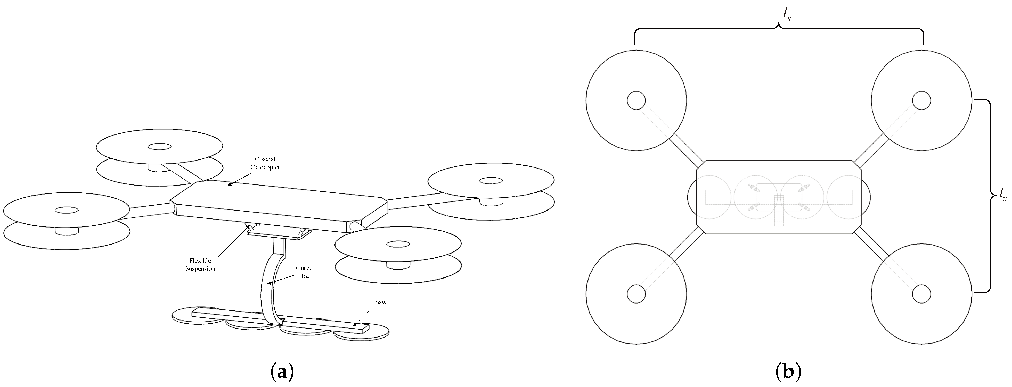
• A coaxial octocopter platform;
• A saw system composed of four pairs of saws;
• A flexible suspension system for buffering damping.

In the overall airframe design, as shown in Figure 4, the saw is connected to the coaxial octocotor by a flexible suspension system. In addition, the configuration of the coaxial octocopter, with eight-power-unit redundancy, can still maintain stability under a certain power failure [18] and has higher reliability and redundancy compared to the quadrotor. At the same time, in order to avoid the influence of the under-rotor wash flow on the tree obstacle cutting, the projection of the Z-axis of the airframe rotor surface to be larger than that of the Z-axis of the saw so that the Y-axis of the airframe is larger than the X-axis length. The relationship between the y-axis length $l_y$ and the x-axis length $l_x$ is $l_y>l_x$.

In response to the problem that the rotor blades may interfere with the tree obstacles during the operation of the drones and cause crashes, the method of the suspended saw is applied. Additionally, in order to solve the problem that the suspended straight bar may interfere with the obstacles of the suspended saw in cutting trees, we improved the suspended straight bar to a suspended curved bar, as shown in Figure 4.

Aiming at the trouble of possible impact force when contacting tree obstacles during drone operation, one approach is to adopt an active flexing method, that is, to overcome the impact force by the active flexing control of the drones [19], but this approach needs to obtain the contact force directly or indirectly, and it is more difficult to obtain the contact force for drones saws and tree obstacles in the practical engineering. Moreover, the problem of the rigidity of the drones themselves has not been solved, and the risk of losing control of the drones is still high.The other approach is to take a passive physical flexibility mechanism, that is, to take a flexible suspension to buffer the impact force of contact [20]. Physical flexibility involves inserting elastic damping units [21] such as springs, torsion springs, and hydraulic dampers into the system and utilizing these elastic units as force and motion transfer units. This method greatly reduces the stiffness of the entire drones, thus making the system itself naturally flexible. Due to the flexibility brought about by the elastic units, in the event of an accident such as a collision, the drones can passively store and absorb the impact energy generated by the collision through the elastic elements, thus protecting the drones’ fuselage and improving the environmental adaptability and safety of the drones [22].

2.2. Control Methods Scheme

In addressing the issue of external reaction forces and moments in contact operations, while flexible suspensions can provide cushioning during drones operation [23], too strong elasticity or too weak damping of flexible suspensions can lead to periodic oscillations. Additionally, the non-rigid structure will bring parameter disturbances and channel coupling interference, which puts higher requirements on the interference suppression performance of the drones controller. Comprehensively, the drone with a flexible suspension structure has to resist the reaction forces and moments during operation in addition to overcoming the additional disturbances brought by non-rigid factors. In order to solve these problems in control, we need to research a control method that has fast convergence capability and is resistant to internal and external disturbances. The traditional PID control structure is simple, but the adjustment of PID parameters relies heavily on experience, and the disturbance suppression ability is limited, making it difficult to achieve the best results. Although LQR control has high accuracy and can achieve the best performance index, it lacks interference resistance and robustness. Active Disturbance Rejection Control (ADRC) consists of three main components: Tracking Differential (TD), Nonlinear State Error Feedback (NLSEF) control law, and an Extended State Observer (ESO) [24]. Although ADRC has better disturbance immunity, its control fastness and convergence need to be strengthened because the ESO’s observation of the coupling term will be directly compensated by the linear compensation to the output of the NLSEF. Traditional sliding-mode control (SMC) [25,26] uses a linear sliding surface. When the system state reaches the sliding surface, the system response becomes insensitive to internal parameter uncertainties and external disturbances, which gives the SMC controller good robustness. Although the control structure of SMC is simple, it suffers from chattering problem and weak disturbance suppression capability. In recent years, terminal sliding-mode control (TSMC) has shown excellent performance in practical applications. For example, the system state error can converge to zero in a finite time, the controller gain can be significantly reduced compared with the linear sliding surface, and the steady-state accuracy is higher than that of the conventional SMC. However, when the system is close to the equilibrium state, the general TSMC method encounters the singularity problem. Therefore, in order to solve the singularity problem, non-singular terminal sliding-mode control (NTSMC) [27] has been proposed, and a variety of improved non-singular terminal sliding-mode control methods have been developed, such as integral non-singular terminal sliding-mode control, fast non-singular terminal sliding-mode control [28], adaptive non-singular terminal sliding-mode control [29], and so on. In this paper, in order to solve the problems of internal parameter perturbations and external contact reaction forces and moments of the TOCCO-FSS, and at the same time to improve the system’s immunity, fastness and robustness [30], the Active Disturbance Rejection Control (ADRC) with strong anti-interference advantages is combined with the Non-Singular Terminal Sliding-Mode Control (NTSMC) with rapidity and robustness, resulting in the Non-Singular Terminal Sliding-Mode Active Disturbance Rejection Control (NTSM-ADRC) algorithm, which is proposed to achieve stable position and attitude control of the TOCCO-FSS.

Summarizing the above scenarios, the work of our research is as follows:

• Propose and model the novel TOCCO-FSS. Moreover, perform overall dynamic modeling using the Lagrange dynamic equation;
• Analyze the effects of contact operations on drones and model contact reaction forces and moments;
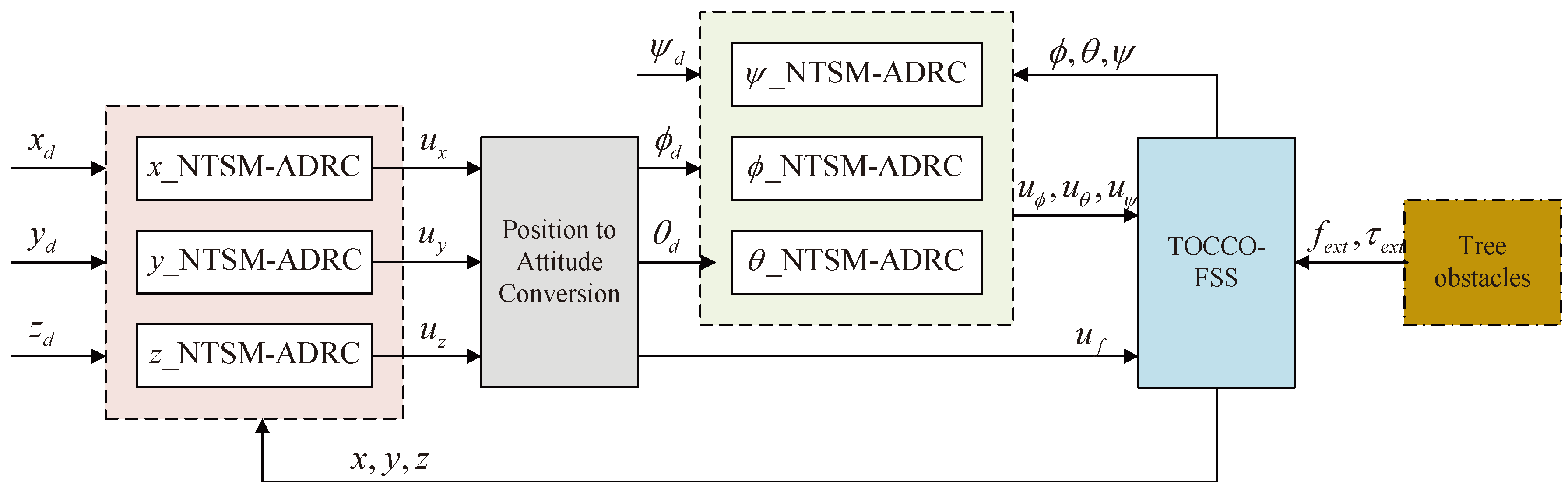
• In response to the perturbations of reaction forces and moments and the TOCCO-FSS internal parameter variations that exist in the contact operation, design the position and attitude control with the Non-Singular Terminal Sliding-Mode Active Disturbance Rejection Control (NTSM-ADRC) and analyze its stability;
• By conducting simulations and physical experiments, the effectiveness of the TOCCO-FSS design, modeling, and control was validated, demonstrating its practical application value.

3. Modeling

The TOCCO-FSS is simplified and a coordinate system is defined as in Figure 5. The airframe consists of a coaxial octocopter, with each pair of rotors spinning in opposite directions on the same axis, and the lift force is directed along the negative of $Z^{\mathrm{B}}$. The Earth coordinate system is ${\mathcal{F}}^{\mathrm{E}}=\left\{O^{\mathrm{E}},X^{\mathrm{E}},Y^{\mathrm{E}},Z^{\mathrm{E}}\right\}$, the airframe coordinate system is ${\mathcal{F}}^{\mathrm{B}}=\left\{O^{\mathrm{B}},X^{\mathrm{B}},Y^{\mathrm{B}},Z^{\mathrm{B}}\right\}$, fixed at the center of mass of the airframe. The saw coordinate system is ${\mathcal{F}}^{\mathrm{S}}=\left\{O^{\mathrm{S}},X^{\mathrm{S}},Y^{\mathrm{S}},Z^{\mathrm{S}}\right\}$, fixed at the center of mass of the saw. Define the length of the saw from the lower end of the flexible suspension system in the airframe coordinate system as ${{\mathit{p}}_l}^{\mathrm{B}}={\left(0,0,p_l\right)}^{\mathrm{T}}$.

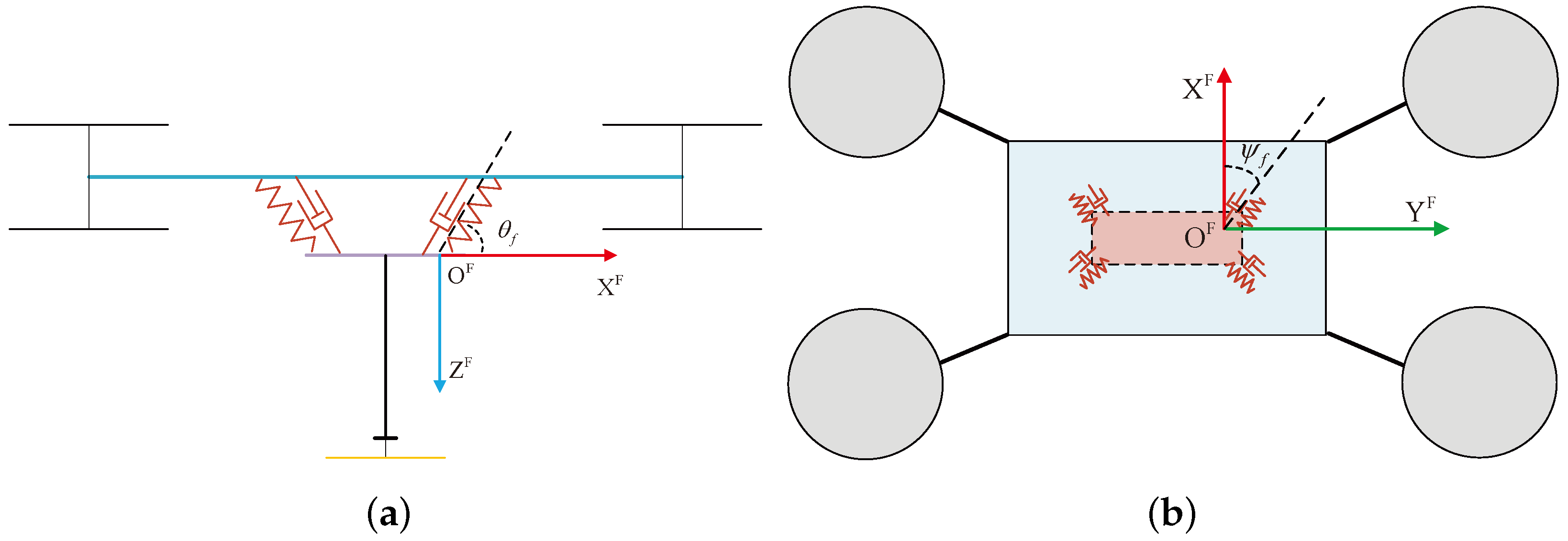
3.1. Flexible Suspension Modeling

The following assumptions are made simultaneously:

• The TOCCO-FSS saw and the airframe are considered to be rigid bodies, and the two parts are connected by a flexible suspension system;
• Due to the relatively light structural weight of the flexible suspension system compared to the body and the saws, its mass can be neglected;
• The flexible suspension system can be equivalently modeled as a three-dimensional spring-damper system in space, and it is connected at the center of mass of the drone. Its front view and top view are shown in Figure 6. It consists of four identical diagonally arranged spring-damper units, which are symmetrically inclined with respect to the XY axes in the body coordinate system;
• Since the saws achieve maximum cutting efficiency when cutting tree obstacles horizontally, the structural design constrains the rotational motion of the flexible suspension system. It provides buffering and vibration damping for translational movements along the XYZ axes in space but does not allow for rotational movement;

To facilitate the calculation, define the flexible coordinate system fixed on the flexible mechanism with positive directions in the X and Y axes as ${\mathcal{F}}^{\mathrm{F}}=\left\{O^{\mathrm{F}},X^{\mathrm{F}},Y^{\mathrm{F}},Z^{\mathrm{F}}\right\}$, shown in Figure 6. So, the rotation angles of the spring-dampers relative to the airframe coordinate system is ${\Omega }_f=\left({\varphi }_f,0,{\psi }_f\right)$. The three-dimensional elastic coefficients ${\mathit{C}}_K^{\mathrm{B}}$ and damping coefficients ${\mathit{C}}_{\xi }^{\mathrm{B}}$ of the flexible suspension system in the body coordinate system can be expressed as the linear superposition of the three-dimensional components of four identical spring-dampers with spring coefficients $C_K$ and damping coefficients $C_{\xi }$, respectively.

$$\left\{\begin{array}{c}{{\mathit{C}}_K}^{\mathrm{B}}=4{\mathit{R}}_{\psi }\left({\psi }_f\right){\mathit{R}}_{\theta }\left({\theta }_f\right){\left[\begin{array}{ccc}{C}_K& 0& 0\end{array}\right]}^{\mathrm{T}}\hfill \\ {{\mathit{C}}_{\xi }}^{\mathrm{B}}=4{\mathit{R}}_{\psi }\left({\psi }_f\right){\mathit{R}}_{\theta }\left({\theta }_f\right){\left[\begin{array}{ccc}{C}_{\xi }& 0& 0\end{array}\right]}^{\mathrm{T}}\hfill \end{array}\right.$$

(1)

where

$${\mathit{R}}_{\theta }=\left[\begin{array}{ccc}\sin \theta & 0& cos\theta \\ 0& 1& 0\\ -cos\theta & 0& \sin \theta \end{array}\right],{\mathit{R}}_{\psi }=\left[\begin{array}{ccc}\sin \psi & -cos\psi & 0\\ cos\psi & \sin \psi & 0\\ 0& 0& 1\end{array}\right]$$

(2)

The coefficient of elasticity is calculated as

$$C_K=\frac{G_k{d}_k^4}{8n_k{D}_k^3}$$

(3)

where $G_k$ is the steel modulus of the spring wire, $d_k$ is the wire diameter of the spring, $n_k$ is the number of coils of the spring, and $D_k$ is the outer diameter of the spring.

Due to the suspension system, this paper adopts the hydraulic damper to accurately establish the model of the hydraulic damper and needs to obtain accurate damper parameters. So, in this paper, from the perspective of engineering applications, according to the experimental parameters, the damping coefficient of the damper can be obtained as

$$C_{\xi }=\frac{W_{\xi }}{V_{\xi }}$$

(4)

where $W_{\xi }$ is the maximum impact force and $V_{\xi }$ is the maximum cushioning velocity.

3.2. Kinematic Modeling

Define the rotation matrix ${\mathit{R}}_E^B$ to denote the rotation relation from the Earth coordinate system to the object coordinate system, the Euler angle of the drone in the Earth coordinate system is ${{\Omega }_b}^{\mathrm{E}}$, the position of the saw in the Earth coordinate system is ${{\mathit{p}}_s}^{\mathrm{E}}$, and the Earth coordinate system Euler angular velocity is converted to the airframe angular velocity matrix as ${\mathit{T}}_b$. Define the generalized coordinate system as $\mathit{q}={\left({{\mathit{p}}_b}^{\mathrm{E}},{{\mathit{p}}_s}^{\mathrm{E}},{{\Omega }_b}^{\mathrm{E}}\right)}^{\mathrm{T}}$.

The linear velocity of the airframe and the saw in the Earth coordinate system is

$$\left\{\begin{array}{c}{{\dot{\mathit{p}}}_b}^{\mathrm{E}}=\left[\begin{array}{ccc}{\mathbf{I}}_{3\times 3}& {\mathbf{0}}_{3\times 3}& {\mathbf{0}}_{3\times 3}\end{array}\right]\dot{\mathit{q}}\hfill \\ {{\dot{\mathit{p}}}_s}^{\mathrm{E}}=\left[\begin{array}{ccc}{\mathbf{0}}_{3\times 3}& {\mathbf{I}}_{3\times 3}& {\mathbf{0}}_{3\times 3}\end{array}\right]\dot{\mathit{q}}\hfill \end{array}\right.$$

(5)

The Euler angular velocity of the airframe and saw in the Earth coordinate system is

$${{\dot{\Omega }}_s}^{\mathrm{E}}={{\dot{\Omega }}_b}^{\mathrm{E}}=\left[\begin{array}{ccc}{\mathbf{0}}_{3\times 3}& {\mathbf{0}}_{3\times 3}& {\mathbf{I}}_{3\times 3}\end{array}\right]\dot{\mathit{q}}$$

(6)

The expansion and contraction of the flexible suspension and the rate of expansion and contraction in the Earth system is

$$\left\{\begin{array}{c}\delta {{\mathit{p}}_k}^{\mathrm{E}}={{\mathit{p}}_s}^{\mathrm{E}}-{{\mathit{p}}_b}^{\mathrm{E}}-{\left({\mathit{R}}_{\mathrm{E}}^{\mathrm{B}}\right)}^{\mathrm{T}}{{\mathit{p}}_l}^{\mathrm{B}}\hfill \\ \delta {{\dot{\mathit{p}}}_k}^{\mathrm{E}}={{\dot{\mathit{p}}}_s}^{\mathrm{E}}-{{\dot{\mathit{p}}}_b}^{\mathrm{E}}-{\left({\dot{\mathit{R}}}_{\mathrm{E}}^{\mathrm{B}}\right)}^{\mathrm{T}}{{\mathit{p}}_l}^{\mathrm{B}}\hfill \end{array}\right.$$

(7)

According to the above equation, the kinematic relationship between the airframe and the tool can be calculated.

3.3. Dynamic Modeling

Since the TOCCO-FSS system consists of an airframe and a flexible suspension saw system, the coupling between the UAV airframe and the flexible suspension is more difficult to deal with when the Newton–Euler method is used to establish the dynamics model of the quadrotor system, and the Lagrange equation modeling is a holistic modeling method from the energy point of view, so this paper adopts the Lagrange equation method for the dynamics modeling. The Lagrange equation can be expressed as

$$\left\{\begin{array}{c}L\left(\mathit{q},\dot{\mathit{q}}\right)=E-U\hfill \\ \frac{d}{dt}\left(\frac{\partial L}{\partial \dot{\mathit{q}}}\right)-\frac{\partial L}{\partial \mathit{q}}+\frac{\partial D}{\partial \dot{\mathit{q}}}=\Gamma \hfill \end{array}\right.$$

(8)

where $\mathit{q}$ is the state quantity, and the generalized coordinate system, E is the total kinetic energy, U is the total potential energy of the system, D is the dissipation function, and $\Gamma$ is the external force.

The total dynamic energy $\mathbf{E}$ is written as

$$\begin{array}{cc}\hfill E& =\frac{1}{2}{m}_b{\left({{\dot{\mathit{p}}}_b}^{\mathrm{E}}\right)}^{\mathrm{T}}{{\dot{\mathit{p}}}_b}^{\mathrm{E}}+\frac{1}{2}{m}_s{\left({{\dot{\mathit{p}}}_s}^{\mathrm{E}}\right)}^{\mathrm{T}}{{\dot{\mathit{p}}}_s}^{\mathrm{E}}+\frac{1}{2}{\left({{\dot{\mathbf{\Phi }}}_b}^{\mathrm{E}}\right)}^{\mathrm{T}}{{\mathit{T}}_b}^{\mathrm{T}}{\mathit{J}}_b{\mathit{T}}_b{{\dot{\mathbf{\Phi }}}_b}^{\mathrm{E}}+\frac{1}{2}{\left({{\dot{\mathbf{\Phi }}}_s}^{\mathrm{E}}\right)}^{\mathrm{T}}{{\mathit{T}}_b}^{\mathrm{T}}{\mathit{J}}_s{\mathit{T}}_b{{\dot{\mathbf{\Phi }}}_s}^{\mathrm{E}}\hfill \\ \hfill & =\frac{1}{2}{\dot{\mathit{q}}}^{\mathrm{T}}\mathit{M}\dot{\mathit{q}}\hfill \end{array}$$

(9)

where

$$\mathit{M}=\left[\begin{array}{ccc}{m}_b{\mathbf{I}}_3& {\mathbf{0}}_{3\times 3}& {\mathbf{0}}_{3\times 3}\\ {\mathbf{0}}_{3\times 3}& m_s{\mathbf{I}}_3& {\mathbf{0}}_{3\times 3}\\ {\mathbf{0}}_{3\times 3}& {\mathbf{0}}_{3\times 3}& {{\mathit{T}}_b}^{\mathrm{T}}\left({\mathit{J}}_b+{\mathit{J}}_s\right){\mathit{T}}_b\end{array}\right]$$

(10)

The total potential energy is

$$U=m_b\mathit{g}{{\mathit{p}}_b}^{\mathrm{E}}+m_s\mathit{g}{{\mathit{p}}_s}^{\mathrm{E}}+\frac{1}{2}{\left(\delta {{\mathit{p}}_k}^{\mathrm{E}}\right)}^{\mathrm{T}}{\left({\mathit{R}}_{\mathrm{E}}^{\mathrm{B}}\right)}^{\mathrm{T}}{\mathit{C}}_K\delta {{\mathit{p}}_k}^{\mathrm{E}}$$

(11)

where $\mathit{g}=\left[\begin{array}{ccc}0& 0& g\end{array}\right]$

The dissipation function is

$$D=\frac{1}{2}{\left(\delta {{\dot{\mathit{p}}}_k}^{\mathrm{E}}\right)}^{\mathrm{T}}{\left({\mathit{R}}_{\mathrm{E}}^{\mathrm{B}}\right)}^{\mathrm{T}}{\mathit{C}}_{\xi }\delta {{\dot{\mathit{p}}}_k}^{\mathrm{E}}$$

(12)

Thus, the Lagrange function can be written as

$$L=E-U=\frac{1}{2}{\dot{\mathit{q}}}^{\mathrm{T}}\mathit{M}\dot{\mathit{q}}-U$$

(13)

The derivative of L is

$$\left\{\begin{array}{c}\frac{\partial L}{\partial \dot{\mathit{q}}}=\frac{\partial E}{\partial \dot{\mathit{q}}}=\mathit{M}\dot{\mathit{q}}\hfill \\ \frac{\partial L}{\partial \mathit{q}}=\frac{1}{2}\frac{\partial }{\partial \mathit{q}}\left({\dot{\mathit{q}}}^{\mathrm{T}}\mathit{M}\dot{\mathit{q}}\right)-{\left(\frac{\partial U}{\partial \mathit{q}}\right)}^{\mathrm{T}}\hfill \\ \frac{d}{dt}\left(\frac{\partial L}{\partial \dot{\mathit{q}}}\right)=\mathit{M}\ddot{\mathit{q}}+\dot{\mathit{M}}\dot{\mathit{q}}\hfill \end{array}\right.$$

(14)

Bringing the above result into the Lagrange equation

$$\mathit{M}\ddot{\mathit{q}}+\dot{\mathit{M}}\dot{\mathit{q}}-\frac{1}{2}\frac{\partial }{\partial \mathit{q}}\left({\dot{\mathit{q}}}^{\mathrm{T}}\mathit{M}\dot{\mathit{q}}\right)+{\left(\frac{\partial U}{\partial \mathit{q}}\right)}^{\mathrm{T}}+\frac{\partial D}{\partial \dot{\mathit{q}}}=\Gamma$$

(15)

Define

$$\mathit{G}={\left(\frac{\partial U}{\partial \mathit{q}}\right)}^{\mathrm{T}},\mathit{C}\left(\mathit{q},\dot{\mathit{q}}\right)\dot{\mathit{q}}=\dot{\mathit{M}}\dot{\mathit{q}}-\frac{1}{2}\frac{\partial }{\partial \mathit{q}}{\left({\dot{\mathit{q}}}^{\mathrm{T}}\mathit{M}\dot{\mathit{q}}\right)}^{\mathrm{T}},\mathit{D}\left(\dot{\mathit{q}}\right)=\frac{\partial D}{\partial \dot{\mathit{q}}}$$

(16)

The Lagrange equation can be organized as

$$\mathit{M}\ddot{\mathit{q}}+\mathit{C}\left(\mathit{q},\dot{\mathit{q}}\right)\dot{\mathit{q}}+\mathit{G}+\mathit{D}=\Gamma$$

(17)

Therefore, the dynamic model can be written as

$$\ddot{\mathit{q}}={\mathit{M}}^{-1}\left[\Gamma -\mathit{C}\left(\mathit{q},\dot{\mathit{q}}\right)\dot{\mathit{q}}-\mathit{G}-\mathit{D}\right]$$

(18)

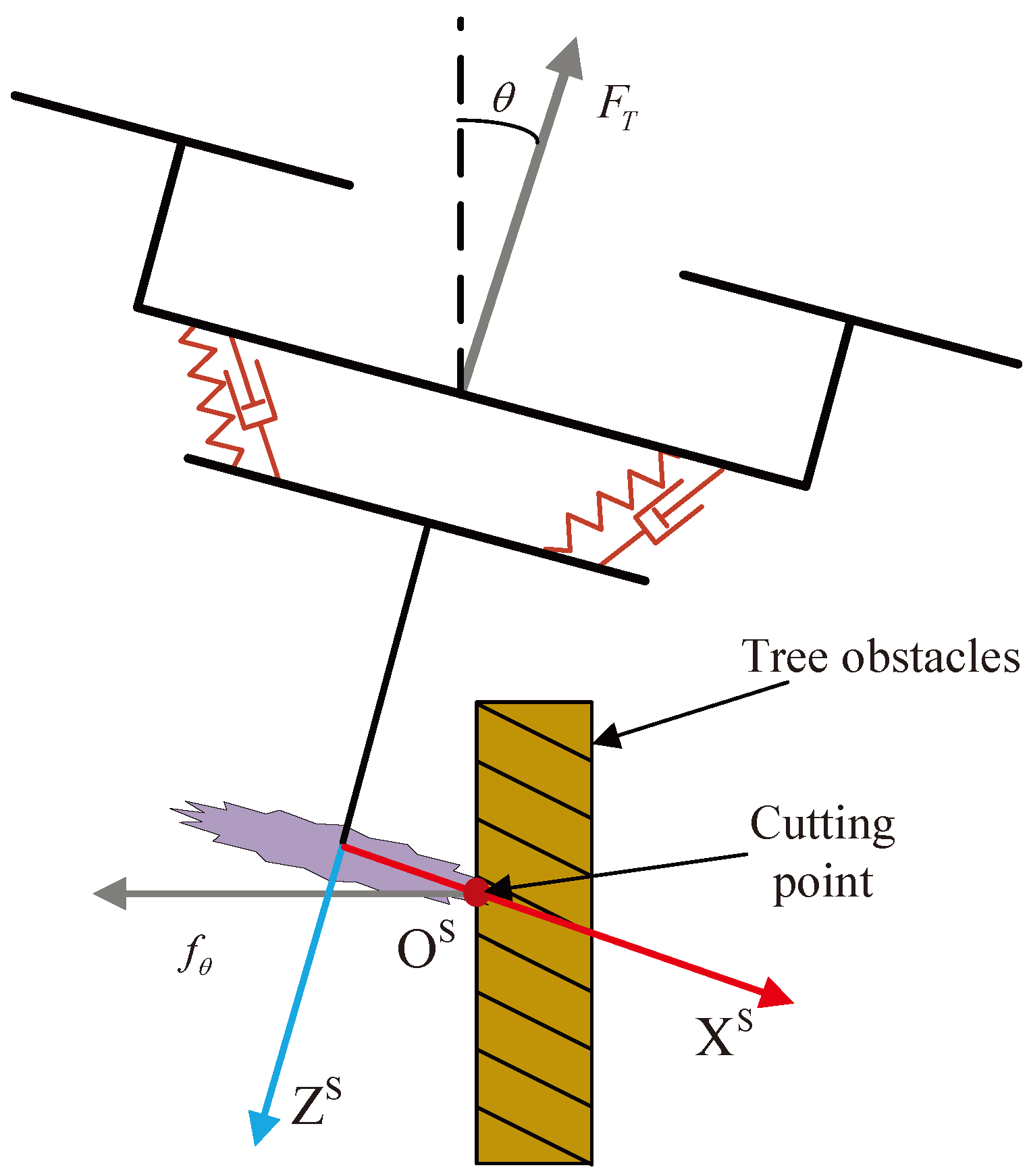
3.4. Contact Operation Modeling

The TOCCO-FSS in this paper has two pairs of circular saws, each pair of which rotates at equal speeds and in opposite rotational directions during operation so that the torque of each pair of saws on the drone can cancel each other out, and even if a combined torque is generated, it can be suppressed by the drone’s heading controller. The disturbance generated by the clearing operation is mainly composed of two parts: the reaction force of the tree barrier on the saws when the knife saws are cutting and the resulting reaction torque, and the resistance and torque generated by the tree barrier on the knife saws, as shown in Figure 7 and Figure 8.

3.4.1. Cutting Disturbance Analysis

The schematic diagram for cutting a tree barrier is shown in Figure 7. When cutting, the tree barrier may be cut by any one of the two pairs of circular saws, and the position of the cutting point corresponding to the coordinate system of the saw is ${\mathit{r}}_f={\left(r_x,r_y,0\right)}^{\mathrm{T}}$. The cutting angle is $\alpha$ and the radius of the circular saw is $r_c$. The resistance to cutting $f_c$ cannot be measured directly, but can be calculated by analyzing the energy. It is generated by the saws cutting the tree, so it is only necessary to obtain the cutting power $P_c$ and the cutting speed $v_c$, which can be calculated as follows:

$$\left\{\begin{array}{c}{f}_c=\frac{P_c}{v_c}\hfill \\ {\mathit{f}}_c={\left[\begin{array}{ccc}-f_c\sin \alpha & -f_{c}cos\alpha & 0\end{array}\right]}^{\mathrm{T}}\hfill \end{array}\right.$$

(19)

The torque generated by a circular saw cutting consists of two parts: rotation with respect to the center of the circular saw and rotation with respect to the origin of the saw’s coordinate system, as follows:

$${\mathit{\tau }}_c={\mathit{r}}_f\times {\mathit{f}}_c+{\left[\begin{array}{ccc}0& 0& -r_c{f}_c\end{array}\right]}^{\mathrm{T}}$$

(20)

3.4.2. Contact Disturbance Analysis

The contact resistance $f_{\theta }$ is related to the pitch angle $\theta$ of the drone, and the relationship between contact resistance and pitch angle is shown in Figure 8.

If the drone slowly contacts the tree obstacle in the air, ignoring the collision with the tree obstacles, when the contact between the drone and the tree obstacle reaches equilibrium, the contact resistance is only related to the pitch attitude of the drone and the thrust ${\mathit{F}}_T$, which is as follows:

$$\left\{\begin{array}{c}{\mathit{f}}_{\theta }=\mathrm{diag}\left(\left[-1,0,0\right]\right){\left({\mathit{R}}_{\mathrm{E}}^{\mathrm{B}}\right)}^{\mathrm{T}}{\mathit{F}}_T\hfill \\ {\mathit{\tau }}_{\theta }={\mathit{r}}_f\times {\mathit{f}}_{\theta }\hfill \end{array}\right.$$

(21)

In summary, combining the above two parts of the disturbances, the final disturbance force and moment can be calculated as

$$\left\{\begin{array}{c}{\mathit{f}}_{ext}={\mathit{f}}_c+{\mathit{f}}_{\theta }\hfill \\ {\mathit{\tau }}_{ext}={\mathit{\tau }}_c+{\mathit{\tau }}_{\theta }\hfill \end{array}\right.$$

(22)

4. Control

The TOCCO-FSS system in this paper experiences significant disturbances during contact operations. To further enhance the disturbance rejection and robustness of the controller, this paper redesigns the state error feedback law using the sliding-mode control method based on the ADRC controller. The overall control system structure is shown in Figure 9.

4.1. Control Output

The relationship between position control and attitude control conversion is given by

$$\left\{\begin{array}{c}{u}_f=\left(m_b+m_s\right)\sqrt{{u_x}^2+{u_y}^2+{u_z}^2}\hfill \\ {\varphi }_d=-{\sin }^{-1}\left(\frac{\left(m_b+m_s\right)\left(u_x\sin \psi -u_{y}cos\psi \right)}{u_f}\right)\hfill \\ {\theta }_d=-{\sin }^{-1}\left(\frac{\left(m_b+m_s\right)\left(u_{x}cos\psi +u_y\sin \psi \right)}{u_f}\right)\hfill \end{array}\right.$$

(23)

where $u_f$ is the final thrust control output, ${\varphi }_d$ is the pitch target control input converted from the X-position channel, and ${\theta }_d$ is the pitch target control ouput converted from the Y-position channel. The relationship between the control output $\left(u_f,u_{\varphi },u_{\theta },u_{\psi }\right)$ converted to the desired speed ${\omega }_i,i=1,2,\dots 8$ is

$$\left[\begin{array}{c}{\omega }_1^2\hfill \\ {\omega }_2^2\hfill \\ {\omega }_3^2\hfill \\ {\omega }_4^2\hfill \\ {\omega }_5^2\hfill \\ {\omega }_6^2\hfill \\ {\omega }_7^2\hfill \\ {\omega }_8^2\hfill \end{array}\right]=\frac{1}{8}\left[\begin{array}{cccc}-1& -1& 1& 1\\ -1& -1& 1& -1\\ -1& -1& -1& -1\\ -1& -1& -1& 1\\ -1& 1& -1& 1\\ -1& 1& -1& -1\\ -1& 1& 1& -1\\ -1& 1& 1& 1\end{array}\right]\mathrm{diag}\left(\frac{1}{c_f},\frac{1}{c_f{l}_y},\frac{1}{c_f{l}_x},\frac{1}{c_d}\right)\left[\begin{array}{c}{u}_f\hfill \\ u_{\varphi }\hfill \\ u_{\theta }\hfill \\ u_{\psi }\hfill \end{array}\right]$$

(24)

where $u_{\varphi }$ is the final roll control output, $u_{\theta }$ is the final pitch control output, $u_{\psi }$ is the final yaw control output.

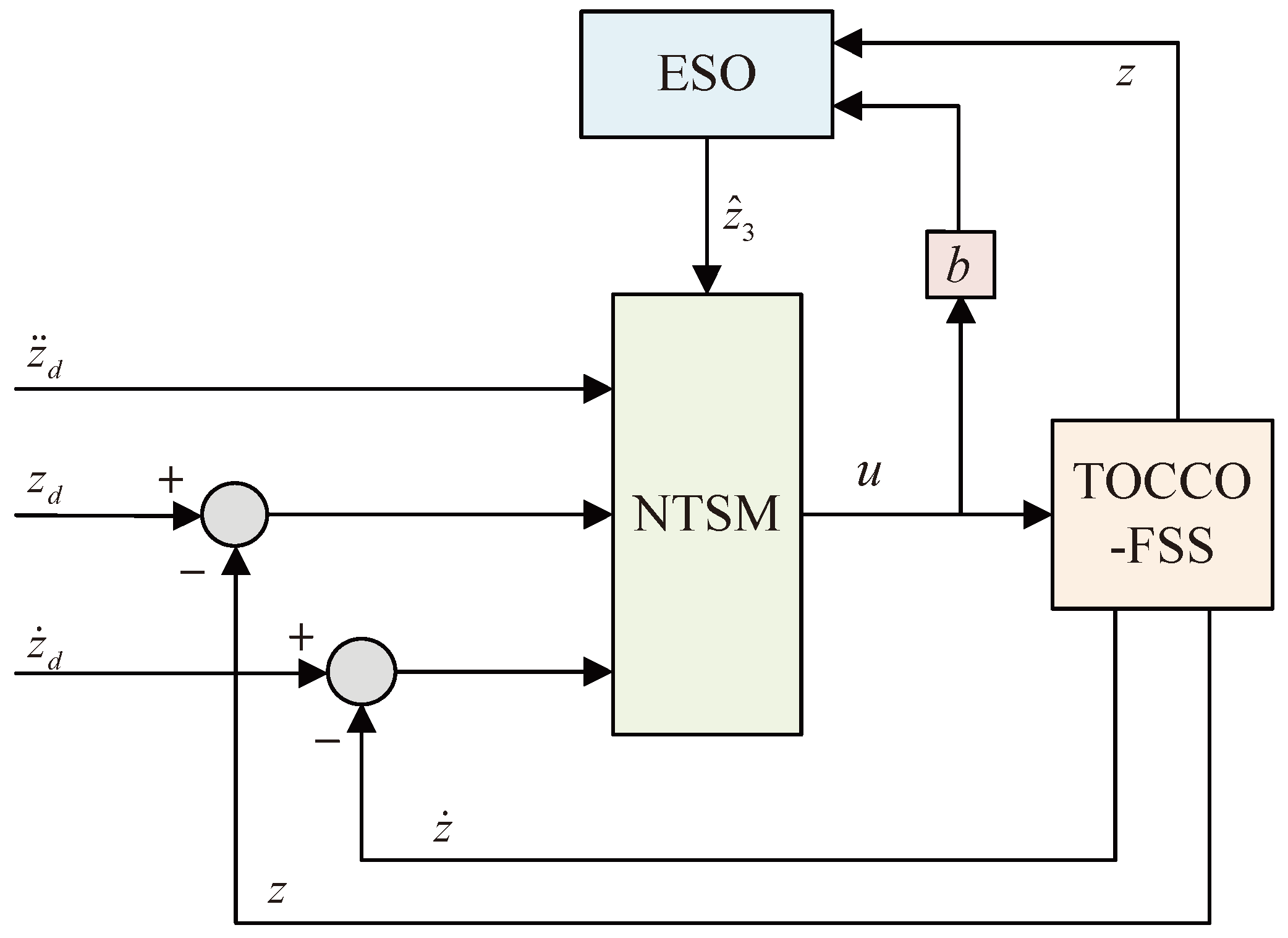
4.2. Extended State Observer

The high-gain error feedback used in the Extended State Observer (ESO) ensures that the dynamics of the observer are much faster than those of the system, effectively making it a fast subsystem of the overall system. This guarantees rapid convergence of the observation error and sufficiently high estimation accuracy, thus providing reliable velocity signals and estimated errors for feedback.

Since the ESO can estimate the total internal and external disturbances of the system, the dynamics model can be rewritten as follows:

$$\left\{\begin{array}{c}{\ddot{p}}_{b,x}=\frac{1}{b_x}{u}_x+f_x\left(t,x,\dot{x},\varphi ,\dot{\varphi },\theta ,\dot{\theta },\psi ,\dot{\psi }\right)\hfill \\ {\ddot{p}}_{b,y}=\frac{1}{b_y}{u}_y+f_y\left(t,y,\dot{y},\varphi ,\dot{\varphi },\theta ,\dot{\theta },\psi ,\dot{\psi }\right)\hfill \\ {\ddot{p}}_{b,z}=\frac{1}{b_z}{u}_z+f_z\left(t,z,\dot{z},\varphi ,\dot{\varphi },\theta ,\dot{\theta },\psi ,\dot{\psi }\right)\hfill \\ {\ddot{\varphi }}_b=\frac{1}{b_{\varphi }}{u}_{\varphi }+f_{\varphi }\left(t,\varphi ,\dot{\varphi },\theta ,\dot{\theta },\psi ,\dot{\psi }\right)\hfill \\ {\ddot{\theta }}_b=\frac{1}{b_{\theta }}{u}_{\theta }+f_{\theta }\left(t,\varphi ,\dot{\varphi },\theta ,\dot{\theta },\psi ,\dot{\psi }\right)\hfill \\ {\ddot{\psi }}_b=\frac{1}{b_{\psi }}{u}_{\psi }+f_{\psi }\left(t,\varphi ,\dot{\varphi },\theta ,\dot{\theta },\psi ,\dot{\psi }\right)\hfill \end{array}\right.$$

(25)

where $b_x=b_y=b_z=\frac{1}{m_b+m_s}$, $b_{\varphi }=\frac{1}{J_{b,x}+J_{s,x}}$, $b_{\theta }=\frac{1}{J_{b,y}+J_{s,y}}$, $b_{\psi }=\frac{1}{J_{b,z}+J_{s,z}}$. $f_i\left(·\right)$ is the disturbance term such as the flexible suspension, channel coupling disturbance, and operational cutting force to which the system is subjected. The extended state observer is designed to realize the estimation and compensation of the uncertainty effects.

By taking the pitch channel as an example, in order to facilitate the observer design, the pitch channel is extended as follows:

$$\left\{\begin{array}{c}{x}_1=\theta \hfill \\ {\dot{x}}_1=x_2\hfill \\ {\dot{x}}_2=x_3+b_{\theta }{u}_{\theta }\hfill \\ {\dot{x}}_3=h\hfill \end{array}\right.$$

(26)

where $x_3$ is the total perturbation of the pitch channel and the derivative ${\dot{x}}_3=h$ exists and is bounded. Then, the form of the ESO can be expressed as

$$\left\{\begin{array}{c}e=x_1-{\widehat{x}}_1\hfill \\ {\dot{\widehat{x}}}_1={\widehat{x}}_2+\frac{{\alpha }_1}{\epsilon }e\hfill \\ {\dot{\widehat{x}}}_2={\widehat{x}}_3+\frac{{\alpha }_2}{{\epsilon }^2}e+b_{\theta }{u}_{\theta }\hfill \\ {\dot{\widehat{x}}}_3=\frac{{\alpha }_3}{{\epsilon }^3}e\hfill \end{array}\right.$$

(27)

where ${\widehat{x}}_i=1,2,3$ is the observed state value of $x_i$ and ${\widehat{x}}_1\left(t\right)\to x_1\left(t\right)$, ${\widehat{x}}_2\left(t\right)\to x_2\left(t\right)$, ${\widehat{x}}_3\left(t\right)\to f_{\theta }\left(t,\theta ,\dot{\theta }\right)$ when $t\to \infty$, where $\epsilon >0$, ${\alpha }_1$, ${\alpha }_2$, ${\alpha }_3$ are positive integers and the polynomial $s^3+{\alpha }_1{s}^2+{\alpha }_{2}s+{\alpha }_3$ satisfies the Hurwitz condition.

4.3. Non-Singular Terminal Sliding-Mode Control

Drones typically use an inner–outer loop control strategy, dividing the six degrees of freedom state variables into the faster-responding inner loop and the slower-responding outer loop. The inner loop is for attitude control, while the outer loop is for position control. The ESO can estimate the coupling terms and total disturbances for each channel, allowing for the design of six-channel NTSM-ADRC controllers.

The controller structure is designed for the altitude channel as an example, combining the dynamics model with the extended state observer and defining the error variables:

$$\left\{\begin{array}{c}{e}_z=z_d-z_1\hfill \\ {\dot{e}}_z={\dot{z}}_d-{\dot{z}}_1\hfill \\ {\ddot{e}}_z={\ddot{z}}_d-{\widehat{z}}_3-b_z{u}_z\hfill \end{array}\right.$$

(28)

where $e_z$ is the error value of the height, ${\dot{e}}_z$ and ${\ddot{e}}_z$ are the first-order and second-order derivative values of the height error, respectively, and $z_d$ is the expected value of the height. ${\widehat{z}}_3$ is the disturbance value estimated by the extended state observer.

Design the non-singular terminal slide model surface as

$$s_z=e_z+\frac{1}{{\beta }_z}{{\dot{e}}_z}^{\frac{p_z}{q_z}}$$

(29)

where ${\beta }_z>0$, $1<\frac{p_z}{q_z}<2$.

Choose the index convergence rate and the non-singular terminal sliding-mode control rate is designed as

$$u_z=\frac{1}{b_z}\left({\ddot{z}}_d-{\widehat{z}}_3+{\beta }_z\frac{q_z}{p_z}{{\dot{e}}_z}^{2-\frac{p_z}{q_z}}+{\omega }_z\mathrm{sgn}\left(s_z\right)+k_z{s}_z\right)$$

(30)

To reduce chattering, the hyperbolic tangent function $\tanh \left(·\right)$ is used to replace the traditional $\mathrm{sgn}\left(·\right)$ function

$$\tanh \left(\frac{s_z}{ϵ}\right)=\frac{e^{\frac{s_z}{ϵ}}-e^{-\frac{s_z}{ϵ}}}{e^{\frac{s_z}{ϵ}}+e^{-\frac{s_z}{ϵ}}}$$

(31)

where $ϵ>0$, and $ϵ$ determines the speed of change of the inflection point of the hyperbolic tangent smooth function. Therefore, the altitude control structure is shown in Figure 10.

Similarly, the control rate of the other channels can be calculated as

$$\left\{\begin{array}{c}{u}_x=\frac{1}{b_x}\left({\ddot{x}}_d-{\widehat{x}}_3+{\beta }_x\frac{q_x}{p_x}{{\dot{e}}_x}^{2-\frac{p_x}{q_x}}+{\omega }_x\tanh \left(s_x\right)+k_x{s}_x\right)\hfill \\ u_y=\frac{1}{b_y}\left({\ddot{y}}_d-{\widehat{y}}_3+{\beta }_y\frac{q_y}{p_y}{{\dot{e}}_y}^{2-\frac{p_y}{q_y}}+{\omega }_y\tanh \left(s_y\right)-k_y{s}_y\right)\hfill \\ u_{\varphi }=\frac{1}{b_{\varphi }}\left({\ddot{\varphi }}_d-{\widehat{\varphi }}_3+{\beta }_{\varphi }\frac{q_{\varphi }}{p_{\varphi }}{{\dot{e}}_{\varphi }}^{2-\frac{p_{\varphi }}{q_{\varphi }}}-{\omega }_{\varphi }\tanh \left(s_{\varphi }\right)-k_{\varphi }{s}_{\varphi }\right)\hfill \\ u_{\theta }=\frac{1}{b_{\theta }}\left({\ddot{\theta }}_d-{\widehat{\theta }}_3+{\beta }_{\theta }\frac{q_{\theta }}{p_{\theta }}{{\dot{e}}_{\theta }}^{2-\frac{p_{\theta }}{q_{\theta }}}-{\omega }_{\theta }\tanh \left(s_{\theta }\right)-k_{\theta }{s}_{\theta }\right)\hfill \\ u_{\psi }=\frac{1}{b_{\psi }}\left({\ddot{\psi }}_d-{\widehat{\psi }}_3+{\beta }_{\psi }\frac{q_{\psi }}{p_{\psi }}{{\dot{e}}_{\psi }}^{2-\frac{p_{\psi }}{q_{\psi }}}-{\omega }_{\psi }\tanh \left(s_{\psi }\right)-k_{\psi }{s}_{\psi }\right)\hfill \end{array}\right.$$

(32)

4.4. Stability Analysis

Analyze the stability of the closed-loop system of NTSM-ADRC. The six-degree-of-freedom channel closed-loop system consists of an expansion observer and a non-singular sliding-mode controller, so the Lyapunov function is defined as $V=V_s+V_o$.

The altitude channel is analyzed as an example, and the remaining channels can satisfy the stability in the Lyapunov sense as long as they satisfy similar conditions.

4.4.1. Analysis of Non-Singular Terminal Sliding-Mode Controller

The Lyapunov function of the sliding-mode surface $s_z$ is chosen as:

$$V_z=\frac{1}{2}{s_z}^2$$

(33)

The derivative is calculated

$$\begin{array}{cc}\hfill {\dot{V}}_z& =s_z{\dot{s}}_z\hfill \\ \hfill & =s_z\left({\dot{e}}_z+\frac{1}{{\beta }_z}\frac{p_z}{q_z}{{\dot{e}}_z}^{\frac{p_z}{q_z}-1}\left({\ddot{z}}_d-{\widehat{z}}_3-b_z{u}_z\right)\right)\hfill \\ \hfill & =\frac{1}{{\beta }_z}\frac{p_z}{q_z}{{\dot{e}}_z}^{\frac{p_z}{q_z}-1}{s}_z\left(-{\omega }_z\mathrm{sgn}\left(s_z\right)-k_z{s}_z\right)\hfill \end{array}$$

(34)

Since $1<\frac{p_z}{q_z}<2$, then $0<\frac{p_z}{q_z}-1<1$, and since ${\beta }_z>0$, $p_z>q_z$ then:

$$\left\{\begin{array}{c}{{\dot{e}}_z}^{\frac{p_z}{q_z}-1}>0\left({\dot{e}}_z\ne 0\right)\hfill \\ s_z{\dot{s}}_z\le \frac{1}{{\beta }_z}\frac{p_z}{q_z}{{\dot{e}}_z}^{\frac{p_z}{q_z}-1}\left(-{\omega }_z\left|s_z\right|\right)=-\frac{1}{{\beta }_z}\frac{p_z}{q_z}{{\dot{e}}_z}^{\frac{p_z}{q_z}-1}{\omega }_z\left|s_z\right|\hfill \end{array}\right.$$

(35)

where $\frac{1}{{\beta }_z}\frac{p_z}{q_z}{{\dot{e}}_z}^{\frac{p_z}{q_z}-1}{\omega }_z>0\left({\dot{e}}_z\ne 0\right)$; therefore, Lyapunov stability is satisfied.

When ${\dot{e}}_z=0$, there is ${\ddot{e}}_z=-{\omega }_z\mathrm{sgn}\left(s_z\right)-k_z{s}_z$. When $s_z>0$, there is ${\ddot{e}}_z\le -{\omega }_z-k_z{s}_z$, and ${\dot{e}}_z$ decreases rapidly; when $s_z<0$, ${\ddot{e}}_z\ge {\omega }_z+k_z{s}_z$, ${\dot{e}}_z$ at this time increases rapidly; and when ${\dot{e}}_z=0$, $s_z=0$ can be realized in a finite time.

4.4.2. Analysis of Extended State Observer

Define

$$\mathit{\eta }={\left[\begin{array}{ccc}{\eta }_1& {\eta }_2& {\eta }_3\end{array}\right]}^{\mathrm{T}}$$

(36)

where ${\eta }_1=\frac{x_1-{\widehat{x}}_1}{{\epsilon }^2}$, ${\eta }_2=\frac{x_2-{\widehat{x}}_2}{\epsilon }$, ${\eta }_3=f\left(t\right)-{\widehat{x}}_3$. There is

$$\left\{\begin{array}{c}\epsilon {\dot{\eta }}_1=\frac{{\dot{x}}_1-{\dot{\widehat{x}}}_1}{\epsilon }=-{\alpha }_1{\eta }_1+{\eta }_2\hfill \\ \epsilon {\dot{\eta }}_2=\epsilon \frac{{\dot{x}}_2-{\dot{\widehat{x}}}_2}{\epsilon }=-{\alpha }_2{\eta }_2+{\eta }_3\hfill \\ \epsilon {\dot{\eta }}_3=\epsilon \left(f\left(t\right)-{\widehat{x}}_3\right)=-{\alpha }_3{\eta }_1+\epsilon \dot{f}\left(t\right)\hfill \end{array}\right.$$

(37)

Thus, the observer error equation of state can be written as

$$\epsilon \dot{\mathit{\eta }}=\widehat{\mathit{A}}\eta +\epsilon \widehat{\mathit{B}}\dot{f}$$

(38)

where

$$\widehat{\mathit{A}}=\left[\begin{array}{ccc}-{\alpha }_1& 1& 0\\ -{\alpha }_2& 0& 1\\ -{\alpha }_3& 0& 0\end{array}\right],\widehat{\mathit{B}}=\left[\begin{array}{c}0\\ 0\\ 1\end{array}\right]$$

(39)

Given any symmetric positive definite matrix $\mathit{Q}$, there exists a symmetric positive definite matrix $\mathit{P}$ satisfying the Lyapunov equation

$${\widehat{\mathit{A}}}^{\mathrm{T}}\mathit{P}+\mathit{P}\widehat{\mathit{A}}+\mathit{Q}=0$$

(40)

Define the Lyapunov function of the observer as

$$V_o=\epsilon {\mathit{\eta }}^{\mathrm{T}}\mathit{P}\mathit{\eta }$$

(41)

Then,

$$\begin{array}{cc}\hfill {\dot{V}}_o& =\epsilon {\dot{\mathit{\eta }}}^{\mathrm{T}}\mathit{P}\mathit{\eta }+\epsilon {\dot{\mathit{\eta }}}^{\mathrm{T}}\mathit{P}\dot{\mathit{\eta }}={\left(\widehat{\mathit{A}}\mathit{\eta }+\epsilon \widehat{\mathit{B}}\dot{f}\right)}^{\mathrm{T}}\mathit{P}\dot{\mathit{\eta }}+{\dot{\mathit{\eta }}}^{\mathrm{T}}\mathbf{P}\left(\widehat{\mathit{A}}\mathit{\eta }+\epsilon \widehat{\mathit{B}}\dot{f}\right)\hfill \\ \hfill & ={\mathit{\eta }}^{\mathrm{T}}\left({\widehat{\mathit{A}}}^{\mathrm{T}}\mathit{P}+\mathit{P}\widehat{\mathit{A}}\right)\mathit{\eta }+2\epsilon {\mathit{\eta }}^{\mathrm{T}}\mathit{P}\widehat{\mathit{B}}\dot{f}\le -{\mathit{\eta }}^{\mathrm{T}}\mathit{Q}\mathit{\eta }+2\epsilon ∥\mathit{P}\widehat{\mathit{B}}∥·∥\mathit{\eta }∥·\left|\dot{f}\right|\hfill \\ \hfill & \le -{\lambda }_{\min }\left(\mathit{Q}\right){∥\mathit{\eta }∥}^2+2\epsilon ∥\mathit{P}\widehat{\mathit{B}}∥·∥\mathit{\eta }∥·\left|\dot{f}\right|\hfill \end{array}$$

(42)

where ${\lambda }_{\min }\left(\mathit{Q}\right)$ is the smallest eigenvalue of $\mathit{Q}$. Thus, the convergence condition for ${\dot{V}}_o\le 0$ is

$$∥\mathit{\eta }∥\le \frac{2\epsilon ∥\mathit{P}\widehat{\mathit{B}}∥·∥\mathit{\eta }∥·\left|\dot{f}\right|}{{\lambda }_{\min }\left(\mathit{Q}\right)}$$

(43)

Therefore, the speed of convergence of the observer error $\mathit{\eta }$ is related to the parameter $\epsilon$, and the smaller $\epsilon$ is, the faster $\mathit{\eta }$ converges. Hence, parameters $\epsilon$ and ${\alpha }_i$ are chosen so that $\widehat{\mathit{A}}$ of the Extended State Observer is a Hurwitz matrix, and there is ${\dot{V}}_o\le 0$. Consequently, the observer error system is boundedly stable. In summary, the stability of the NTSM-ADRC is demonstrated.

5. Experiment

In the experimental chapter, we have performed simulation and physical tree-cutting experiments, the simulation study includes the content as shown in

Table 1. The experimental content and purpose for the experiment.

Experimental Content	Purpose
Attitude Control Experiment	Verification of the effect of using different control methods on attitude control under elasticity, rigidity and spring-damping
Position Control Experiment	Verification of the effect of using different control methods on position control under elasticity, rigidity and spring-damping
Flexible Coefficient Experiment	Verification of the effect of different elastic-damping coefficients on position
Contact Operation Experiment	Verification of the effect of using different control methods on contact operation
Pyhsical Experiment	Validation of the effectiveness of TOCCO-FSS in practical applications

.

5.1. Simulation

The TOCCO-FSS system is constructed in the simulation environment, and the simulation parameters of the TOCCO-FSS system are shown in

Table 2. The simulation parameters of the TOCCO-FSS system.

Parameters	Value	Unit
Airframe quality, $m_b$	20.2	kg
Airframe width, $l_y$	2.5	m
Airframe length, $l_x$	1.5	m
Inertia tensor of airframe in x-axis, $J_{b,x}$	4.2	$\mathrm{kg}·{\mathrm{m}}^2$
Inertia tensor of airframe in y-axis, $J_{b,y}$	2.5	$\mathrm{kg}·{\mathrm{m}}^2$
Inertia tensor of airframe in z-axis, $J_{b,z}$	3.2	$\mathrm{kg}·{\mathrm{m}}^2$
Lift coefficient, $C_f$	$1.4\times {10}^{-4}$	$\mathrm{N}·{\mathrm{rad}}^{-2}$
Antitorque coefficient, $C_d$	$2.5\times {10}^{-6}$	$\mathrm{N}·\mathrm{m}·{\mathrm{rad}}^{-2}$
Saw hanging lengths, $l_s$	1.5	m
Saw quality, $m_s$	5.15	kg
Inertia tensor of saw in x-axis, $J_{s,x}$	2.2	$\mathrm{kg}·{\mathrm{m}}^2$
Inertia tensor of saw in y-axis, $J_{s,y}$	1.1	$\mathrm{kg}·{\mathrm{m}}^2$
Inertia tensor of saw in z-axis, $J_{s,z}$	1.6	$\mathrm{kg}·{\mathrm{m}}^2$
Roll angle of flexible suspension, ${\varphi }_f$	60	deg
Yaw angle of flexible suspension, ${\psi }_f$	45	deg
Steel modulus of the spring, $G_k$	8000	MPa
Number of coils of the spring, $n_k$	20	−
Outer diameter of the spring, $D_k$	35	mm
Wire diameter of the spring, $d_k$	2.5	mm
Maximum impact force of the damper, $W_{\xi }$	500	N
Maximum velocity of the damper, $V_{\xi }$	10	$\mathrm{m}/\mathrm{s}$

.

Based on the parameters of the system, and several fine-tunings, the final control system parameters are shown in

Table 3. The control parameters of the TOCCO-FSS system.

	Parameters	$\mathit{\varphi }$	$\mathit{\theta }$	$\mathit{\psi }$	x	y	z
ESO	$\epsilon$	0.01	0.01	0.01	0.05	0.05	0.02
	${\alpha }_1$	6	6	6	3	3	6
	${\alpha }_2$	11	11	11	5	5	10
	${\alpha }_3$	6	6	6	3	3	6
tanh	$ϵ$	0.01	0.01	0.01	0.1	0.1	0.1
NTSM	$\beta$	3	3	3	1.5	1.5	4
	p	5	5	5	5	5	5
	q	3	3	3	3	3	3
	$\omega$	5	5	5	3	3	6
	k	8	8	8	5	5	10

:

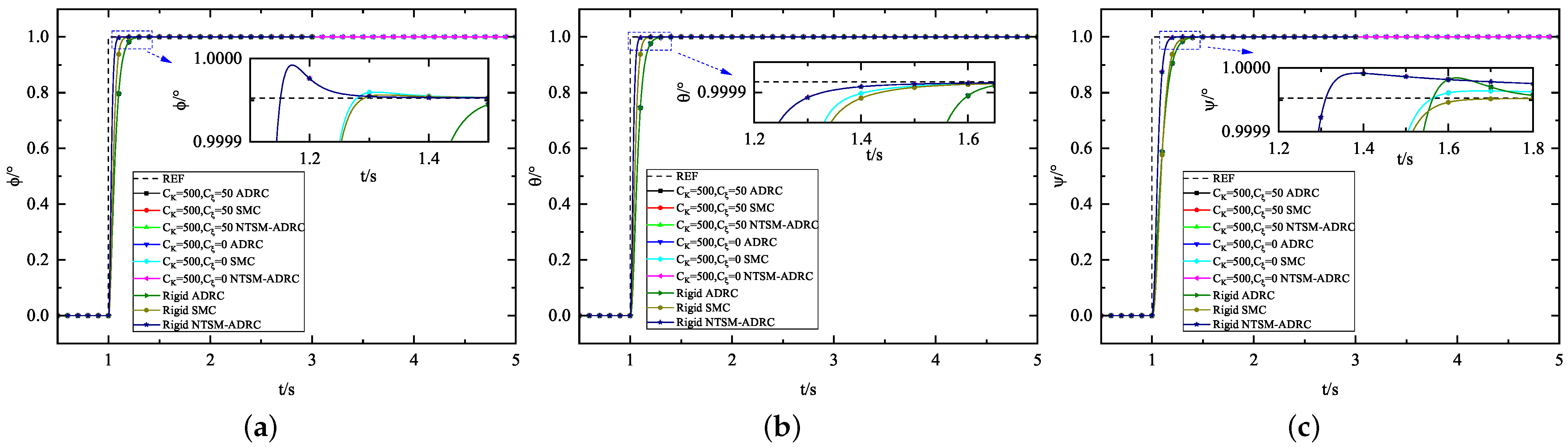
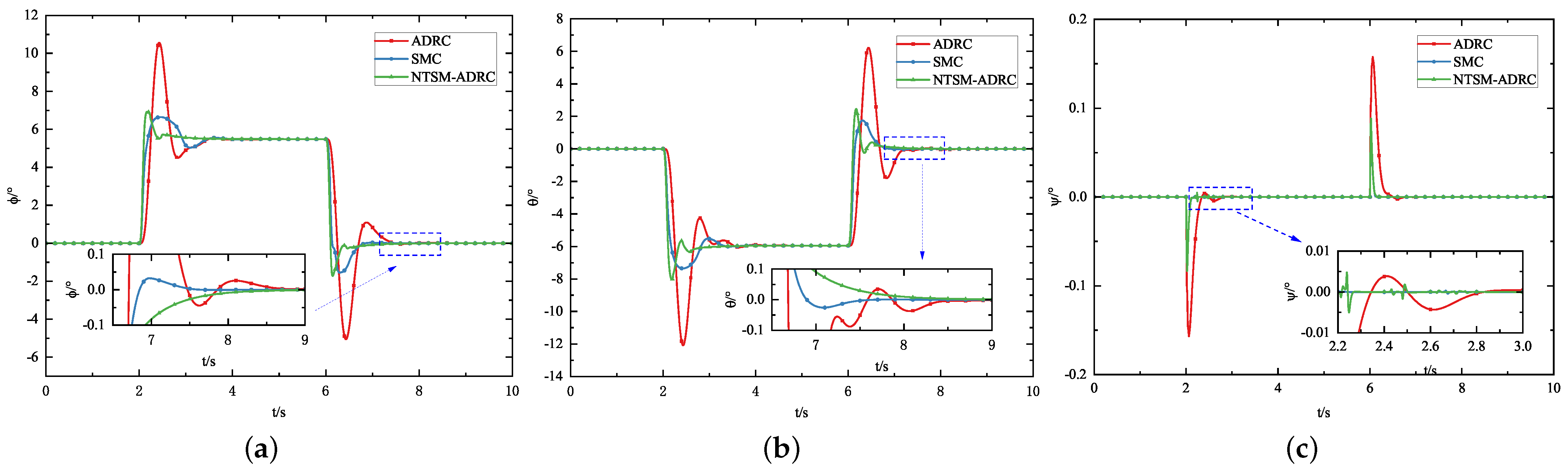
5.1.1. Attitude Control Experiment

Firstly, the ADRC, SMC, and NTSM-ADRC were employed for attitude control comparison; at 1 s, the target three-axis attitude angle is set to 1°. Through calculations, the spring coefficient is approximately $500\mathrm{N}/\mathrm{m}$, and the damping coefficient is approximately $50\mathrm{N}·\mathrm{m}/\mathrm{s}$. Three sets of experiments are set up: with spring-damper, with only spring, and with rigid connection; the simulation results are shown in Figure 11.

From the simulation results shown in Figure 11, the NTSM-ADRC reaches the desired attitude quickly for different flexibility coefficients. The SMC is slightly slower than the NTSM-ADRC, and the ADRC is the slowest to reach the desired point. Additionally, in whichever controller, the attitude loop of the TOCCO-FSS is minimally affected by the flexible suspension system with different elastic and damping coefficients. Thus, in attitude control, NTSM-ADRC reaches the desired angle faster than ADRC and SMC, with quicker convergence and better responsiveness, and SMC performes a little better than ADRC. Therefore, NTSM-ADRC performs better in attitude control compared to ADRC and SMC.

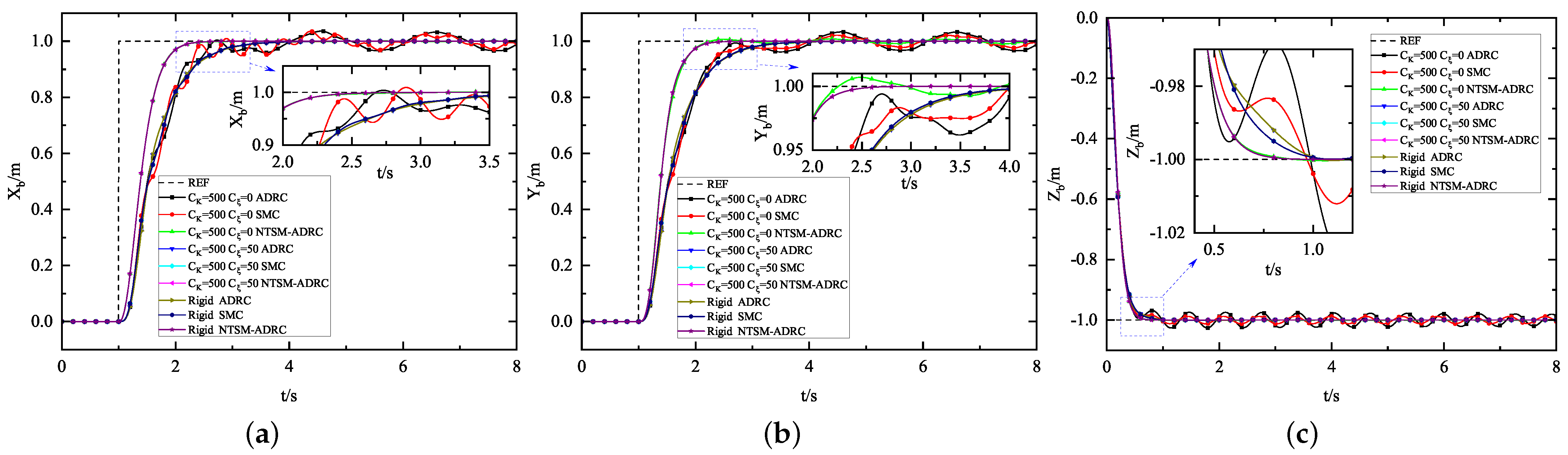
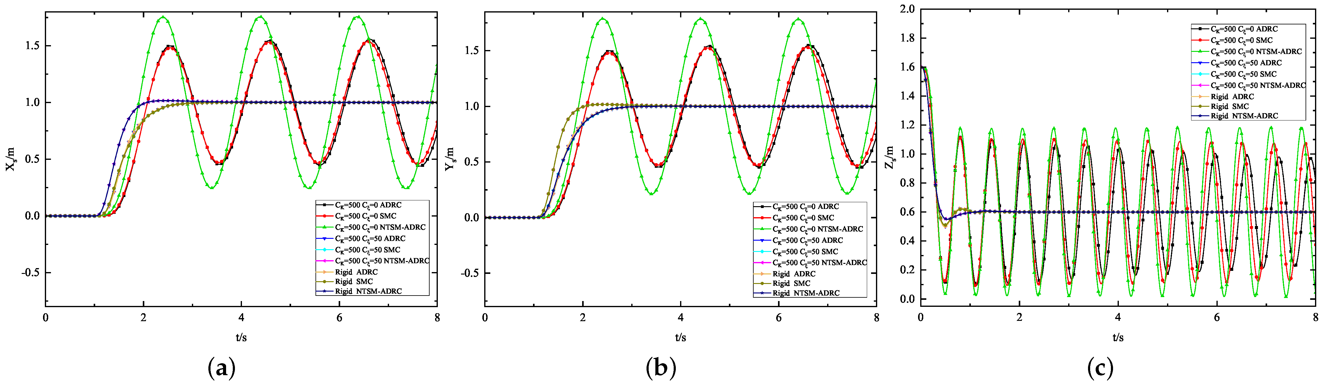
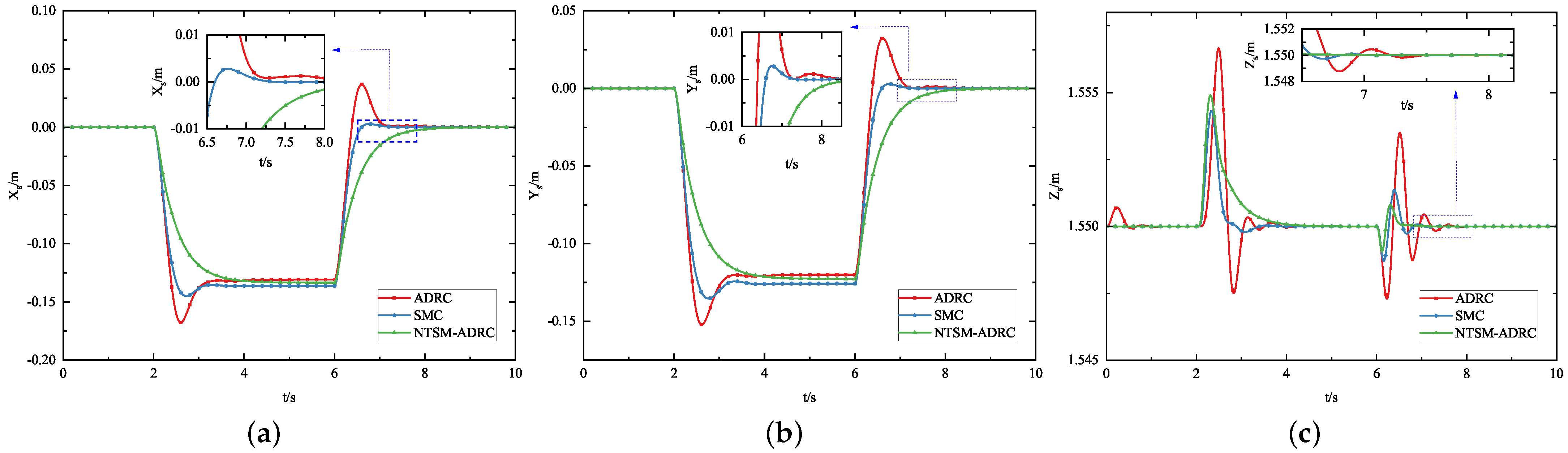
5.1.2. Position Control Experiment

In this section, ADRC, SMC, and NTSM-ADRC were employed for position control comparison; the selection of elastic and damping coefficients is the same as in attitude control. First, set the desired Z position to 1 m. At 1 s, set the desired XY position to 1 m. The simulation results of the airframe and saw are shown in Figure 12 and Figure 13.

In Figure 12 and Figure 13, it can be seen that the flexible structure significantly affects the position of the TOCCO-FSS. The smaller the elastic coefficient, the greater the oscillation of the TOCCO-FSS’s saw. Additionally, in terms of body position control, NTSM-ADRC demonstrates better stability compared to ADRC and SMC. The airframe can still converge quickly under rigid elastic-damping and pure elastic conditions, while the ADRC-controlled and SMC-controlled airframe experiences varying degrees of oscillations and even equal amplitude oscillations under pure spring action. This indicates that NTSM-ADRC has better disturbance rejection and robustness than ADRC and SMC. Under pure spring action, the saw experiences equal amplitude oscillations under NTSM-ADRC, ADRC, and SMC. This is due to the lack of damping, which prevents the release of elastic potential energy. Therefore, the spring-damping system is crucial for the stability of the TOCCO-FSS. Without damping, the elastic potential energy of the TOCCO-FSS cannot be dissipated, leading to a risk of losing control. Moreover, the saw oscillations under NTSM-ADRC control are larger than those of ADRC and SMC, which can be explained from the point of view of energy, as it can be seen from the Lagrange equation that the total energy of the system is certain, and the energy accumulated by the spring, which cannot be released from the airframe, will inevitably be released from the saw in the process of the motion, whereas the airframe under the control of ADRC and SMC will release a part of the energy from the airframe due to its weaker stability, and the the airframe under NTSM-ADRC control has better stability, so the energy can only be released through the saw.

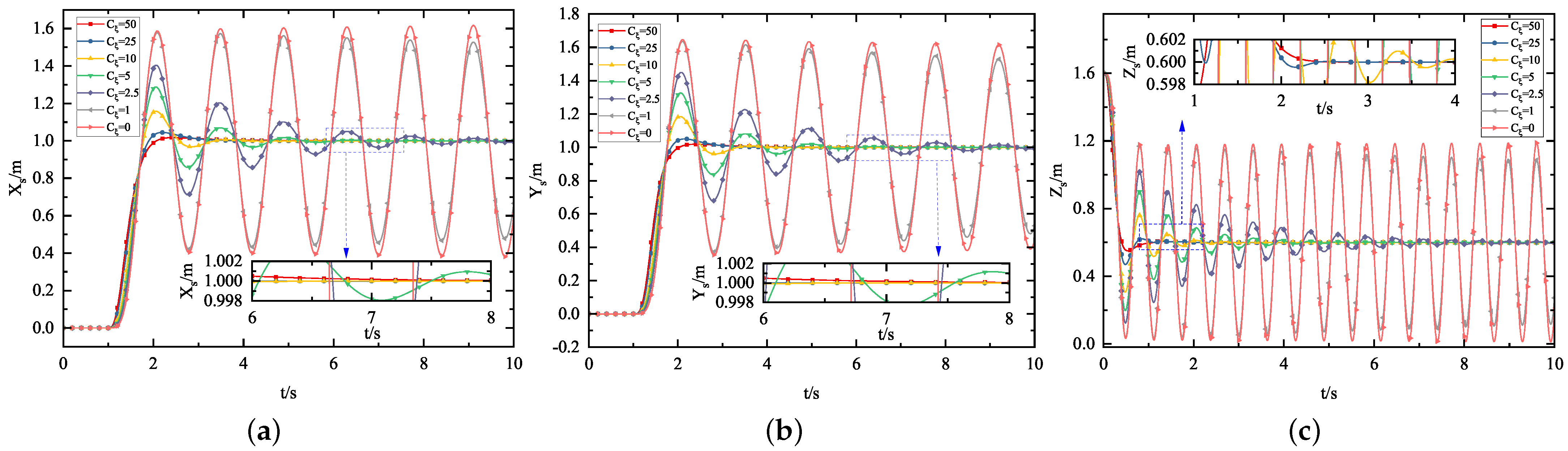
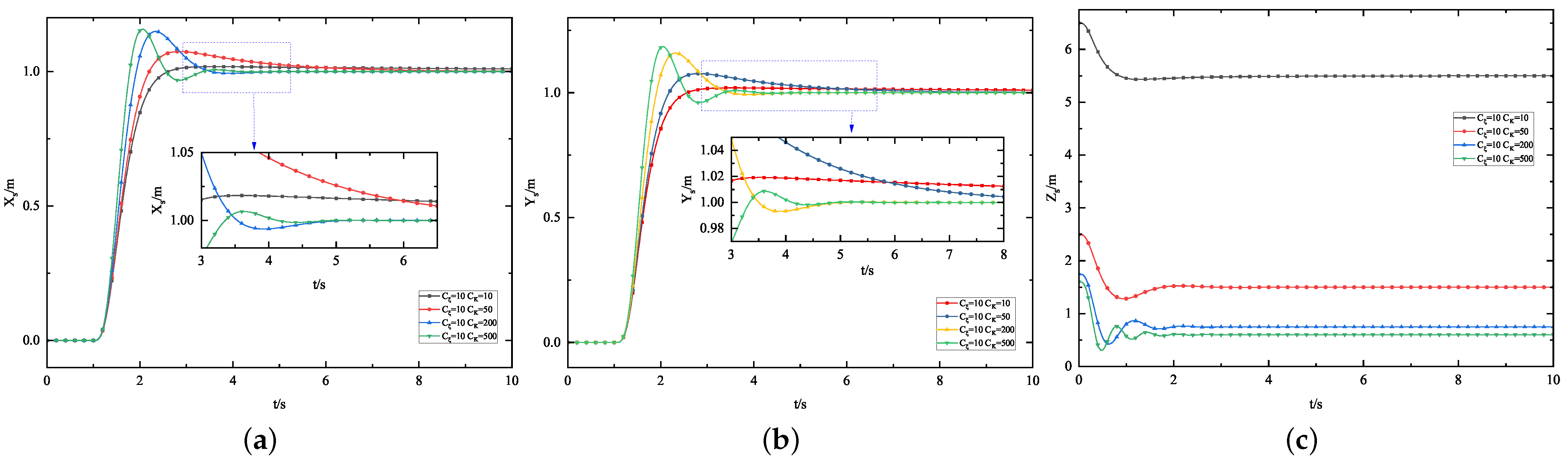
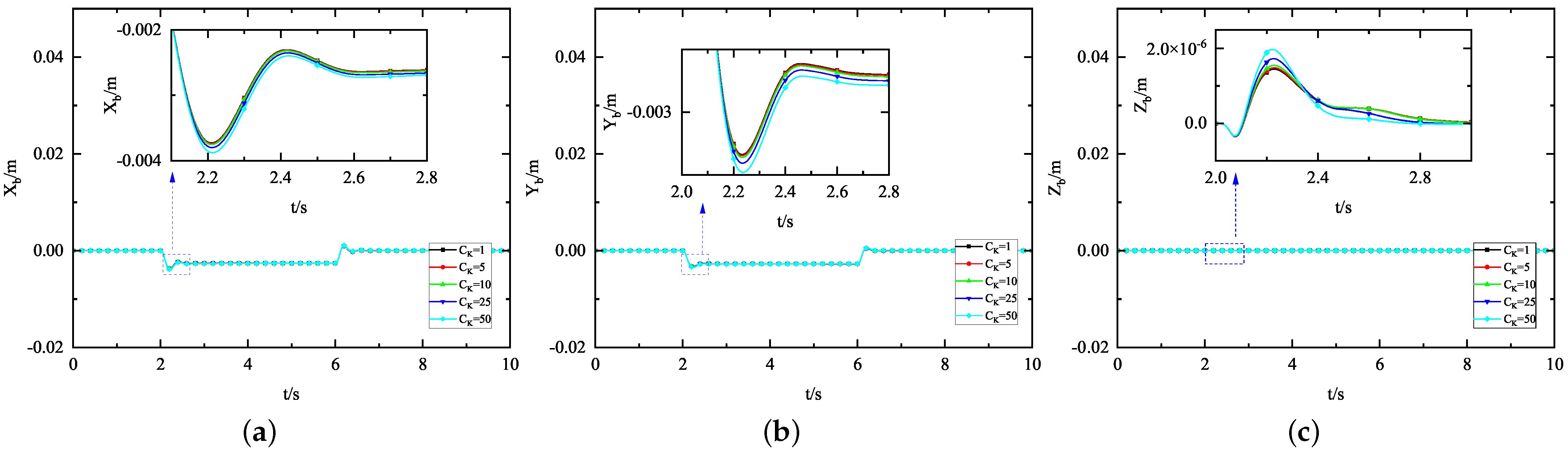
5.1.3. Flexible Coefficient Experiment

To further investigate the impact of the spring-damping system on the TOCCO-FSS, we conducted a series of experiments and simulations. Different damping coefficients and different elastic coefficients are selected to test the impact of coefficients on the stability of the saw. First, we selected the normal elastic coefficient of $C_K=500\mathrm{N}/\mathrm{m}$ and varied the damping coefficient $C_{\xi }$ to study its effect on the stability of the saw. The experimental results are shown in Figure 14 and Figure 15.

In Figure 14, it can be seen that with a constant spring coefficient, different damping coefficients have a significant impact on the saw’s stability. When the damping coefficient is $C_{\xi }=50$, the saw exhibits almost no oscillation. As the damping coefficient decreases, the oscillation amplitude of the saw increases. When the damping coefficient is $C_{\xi }=0$, the saw experiences sustained oscillations of equal amplitude. The reason for this is that the elastic potential energy of the spring cannot be dissipated. It is worth noting that under different damping coefficients, since the spring coefficient remains constant, the oscillation period is consistent.

Then, we select the normal damping coefficient of $C_{\xi }=10\mathrm{N}·\mathrm{m}/\mathrm{s}$ and change the elastic coefficient $C_K$ to study its effect on the stability of the saw. The experimental results are shown in Figure 15.

In Figure 15, it can be seen that with a constant damping coefficient, the smaller the elastic coefficient, the smaller the oscillation amplitude of the saw but the longer the convergence time. At the same time, the smaller the elastic coefficient, the more the saw’s Z-axis equilibrium position is extended due to gravity.

In summary, a smaller elastic coefficient, which means a softer spring and more flexible suspension, will reduce oscillations but increase the delay in following the body, and the Z-axis spring will be more easily extended. The damper is also crucial for the flexible suspension. The smaller the damping coefficient, the harder it is to eliminate the saw’s oscillations. The larger the damping coefficient, the better the oscillations of the saw are absorbed and suppressed. However, a larger damping coefficient means a larger size and weight of the damper. Therefore, from a practical engineering perspective, it is necessary to reasonably select the damping coefficient and elastic coefficient based on the size and weight of the airframe and the saw.

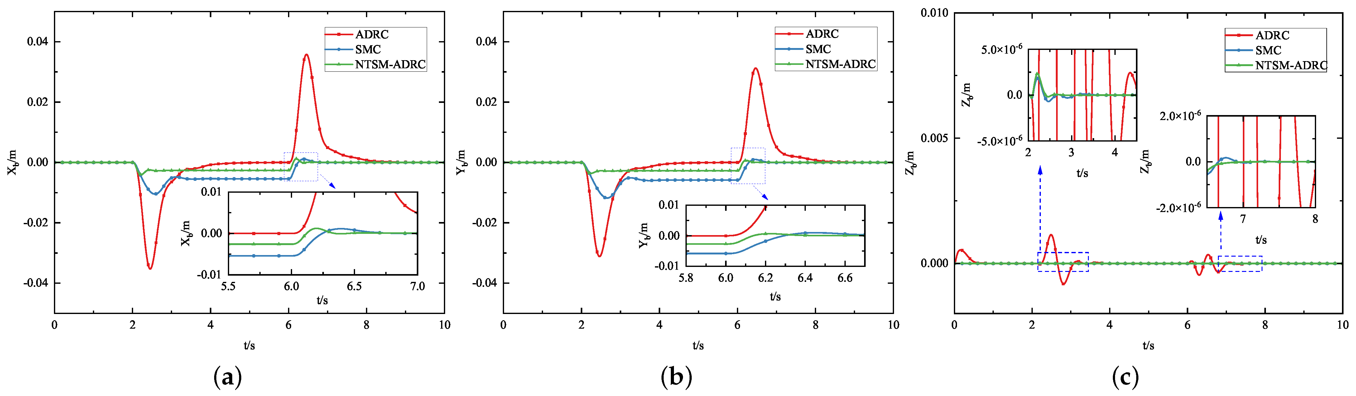
5.1.4. Contact Operation Experiment

Assume that at 2 s, the tree cutting begins with a 5° pitch angle. The cutting position is ${\mathit{r}}_c=\left(0.5\mathrm{m},0.1\mathrm{m},0\right)$, the cutting angle is $\alpha ={45}^{\circ }$, the cutting power is 250 W, the cutting radius is 0.2 m, and the cutting speed is $3000\mathrm{r}·{\min }^{-1}$. The cutting operation is completed at 8 s. The total disturbance force and torque generated are given by Equation (44).

$$\left\{\begin{array}{c}{\mathit{f}}_{ext}=\left[\begin{array}{c}\left(-24-25\times \sin 5^{\circ }\right)\left(\delta \left(t-8\right)-\delta \left(t-2\right)\right)\\ -24\left(\delta \left(t-8\right)-\delta \left(t-2\right)\right)+10\sin 5t\\ 0\end{array}\right]\hfill \\ \begin{array}{cc}\hfill {\mathit{\tau }}_{ext}& =\left[\begin{array}{c}\left(-24-25\times \sin 5^{\circ }\right)\left(\delta \left(t-8\right)-\delta \left(t-2\right)\right)\\ -24\left(\delta \left(t-8\right)-\delta \left(t-2\right)\right)\end{array}\right]\times \left[\begin{array}{c}0.5\\ 0.1\\ 0\end{array}\right]\hfill \\ \hfill & +\left[\begin{array}{c}0\\ 0\\ \left(-24\times 0.2\right)\left(\delta \left(t-8\right)-\delta \left(t-2\right)\right)\end{array}\right]\hfill \end{array}\hfill \end{array}\right.$$

(44)

The simulation results are shown in Figure 16, Figure 17, Figure 18, Figure 19 and Figure 20. In these figures, the influence of contact disturbances can be seen. Under the external force, the position under NTSM-ADRC drifted by a small amount, the position under SMC drifted by a slightly larger amount, and the position under ADRC drifted by a large amount relative to NTSM-ADRC and SMC. The steady-state error is smaller in the presence of disturbances, and the system can quickly return to its original position after the disturbance disappears under NTSM-ADRC. So, NTSM-ADRC provides better control performance compared to SMC and ADRC. Since ADRC and NTSM-ADRC have observers and SMC does not, SMC is not included in the disturbance estimation in Figure 19 and Figure 20, and it can be seen that NTSM-ADRC converges faster to the disturbance estimation with less oscillation. Additionally, from the saw position change curve in Figure 17, it can be observed that with the buffering provided by the flexible suspension system, the position of the saw changes gradually and does not experience abrupt shifts due to disturbance impacts. This buffering effect of the flexible suspension reduces the impact of contact disturbances on the airframe during saw operation. Additionally, because of the better airframe position and attitude control under NTSM-ADRC, the saw changes more slowly and its buffering is better.

5.1.5. Contact Operation Experiment with Different Flexible Coefficients

To further investigate the impact of the spring-damping coefficients of the flexible suspension system on the TOCCO-FSS during contact operations, we conduct experiments with different spring-damping coefficients. First, we keep the damping coefficient constant at $C_{\xi }=50$ while varying the elastic coefficient. The experimental results are shown in Figure 21 and Figure 22.

In Figure 21 and Figure 22, it can be seen that with a constant damping coefficient, the smaller the elastic coefficient, the greater the extension of the load saw when subjected to external forces during contact operations. As seen in Figure 22, when $C_k=50$, the distance stretched by the saw under the external force is only about 0.2 m. When $C_k=1$, the elasticity coefficient is very small, and the flexible suspension is more easily stretched, so it will produce a stretching distance of about 1 m under the action of the external force. Although $C_k=1$ is not possible in practice, the effect of different elasticity coefficients on the system can be obtained through simulation analysis. Thus, a weaker coefficient of elasticity indicates less rigidity and more buffering capacity. However, it can also be seen from Figure 22 that the weaker the coefficient of elasticity, the slower the recovery after the external force disappears.

Next, we varied the damping coefficient $C_{\xi }$. The experimental results are shown in Figure 23 and Figure 24.

In Figure 23 and Figure 24, it can be seen that with a constant elastic coefficient, the stretching length is determined by the elastic coefficient. The smaller the damping coefficient, the greater the oscillation of the load saw when subjected to external forces during contact operations, resulting in weaker buffering capability. Conversely, the larger the damping coefficient, the better the buffering capability, leading to a smoother process of reaching the equilibrium position, although this process takes longer.

In summary, the combined spring-damping coefficient determines the buffering effect of the flexible suspension system. A larger elastic coefficient results in shorter buffering distances, increased rigidity, and weaker buffering capability. Conversely, a smaller elastic coefficient leads to excessively long buffering distances. A larger damping coefficient enhances the ability to suppress spring oscillations and prolongs the buffering time, but the size of the damper is proportional to the damping coefficient, making it impractical to increase indefinitely in actual engineering. Therefore, in practical engineering, the spring-damping coefficients of the flexible suspension structure need to be selected based on the comprehensive parameters of the system.

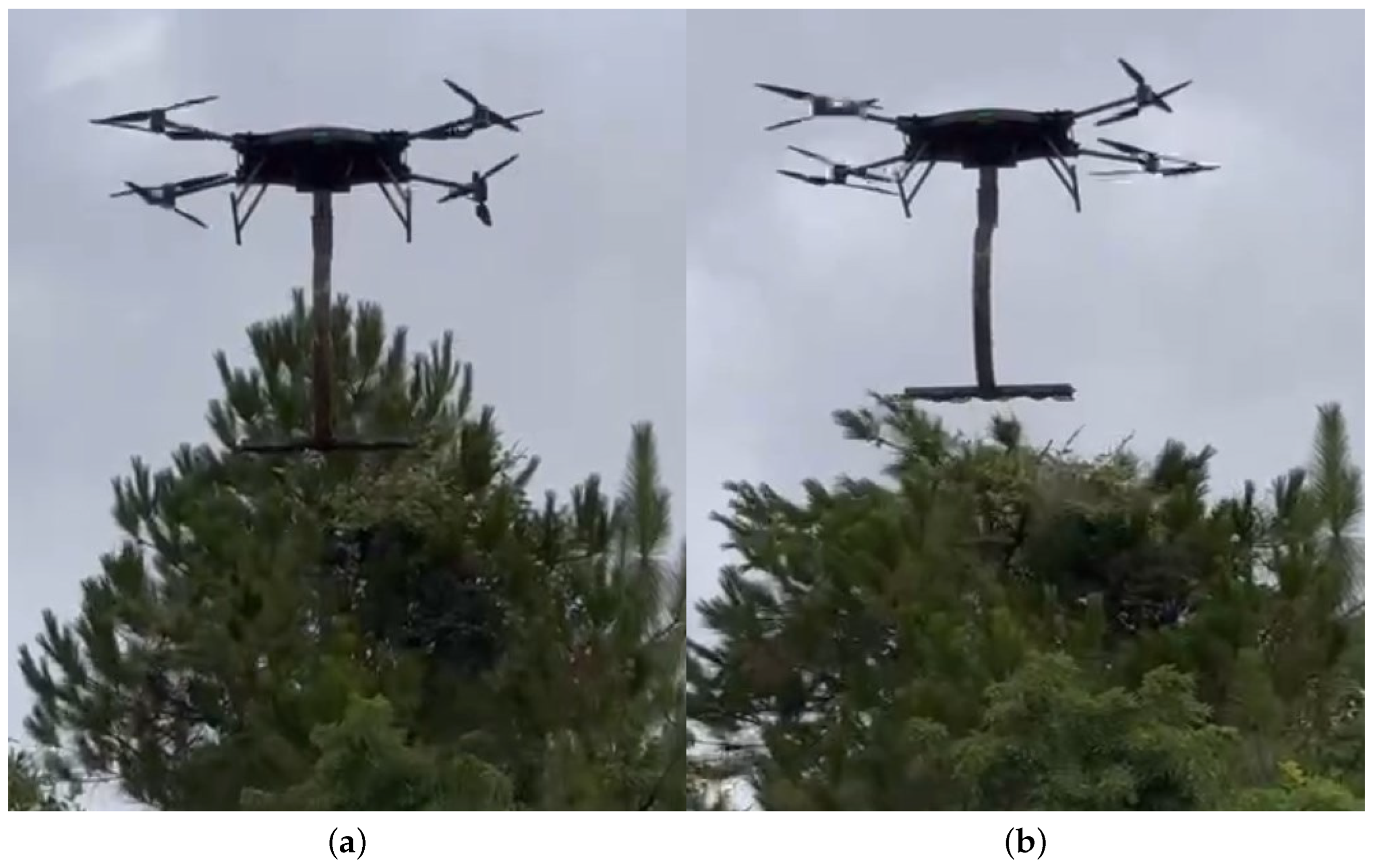
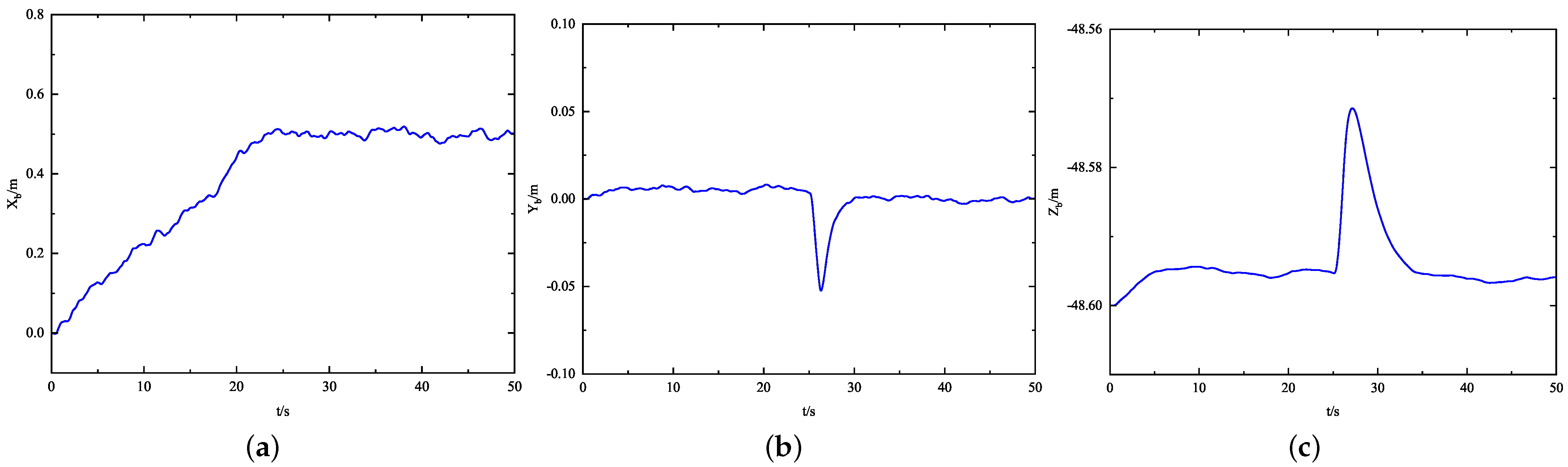
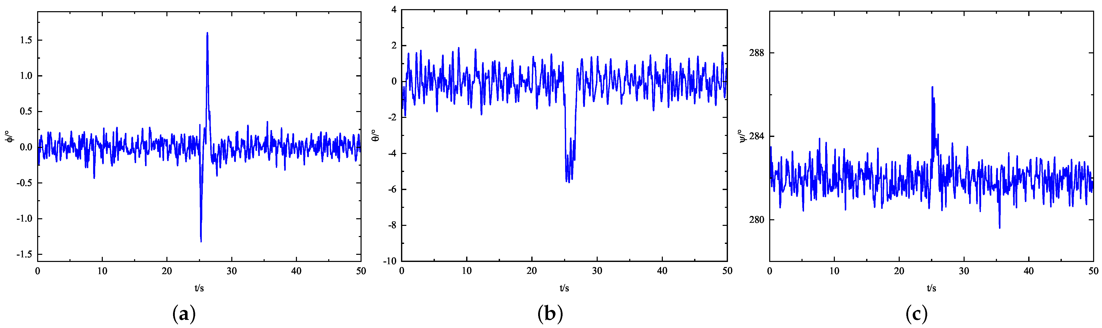
5.2. Physical Experiment

Based on the modeling and simulation, we built a physical TOCCO-FSS prototype, which includes a coaxial octocopter platform, a flexible suspension mechanism, and a saw system. The airframe and saw are constructed from carbon fiber and aluminum alloy. The flexible suspension system consists of hydraulic buffer springs that integrate both spring and damping functions. The flight controller hardware system uses a self-developed flight control hardware, with a UBLOX dual F9P RTK positioning system. The flight control unit has a built-in SD card module for recording flight data. Some of the physical parameters of the TOCCO-FSS system are shown in

Table 4. Some of the physical parameters of the TOCCO-FSS system in practical application.

Parameters	Value	Unit
Airframe quality, $m_b$	25	kg
Saw quality, $m_s$	6.2	kg
Suspension saw lengths, $l_s$	1.5	m
Airframe width, $l_y$	2.5	m
Airframe length, $l_x$	1.5	m
Steel modulus of the spring, $G_k$	8000	MPa
Number of coils of the spring, $n_k$	20	−
Outer diameter of the spring, $D_k$	35	mm
Wire diameter of the spring, $d_k$	2.5	mm
Maximum impact force of the damper, $W_{\xi }$	500	N
Maximum velocity of the damper, $V_{\xi }$	10	$\mathrm{m}/\mathrm{s}$
Roll angle of flexible suspension, ${\varphi }_f$	60	deg
Yaw angle of flexible suspension, ${\psi }_f$	45	deg
Rotor size	32	inch
Battery voltage	54	V

.

The actual tree cutting experiment was conducted outdoors, as shown in Figure 25. In the actual tree obstacle-cutting scenario, the TOCCO-FSS moves at nearly constant speed to the tree obstacle, then begins cutting at a pitch angle of approximately 5°. The flight data recorded during this period are shown in Figure 26 and Figure 27.

In Figure 26 and Figure 27, at approximately 25 seconds, the TOCCO-FSS contacted the tree obstacle and began cutting. During this period, the pitch angle changed by about 5°, and the roll and yaw angles experienced momentary disturbances due to the contact operation but quickly stabilized. After approximately 2 seconds, the tree obstacle was cleared, and the TOCCO-FSS swiftly returned to normal operation, maintaining good stability throughout.

Then, we cleared different types of tree obstacles, sampling different cut-down tree obstacles. The maximum diameter of the different tree obstacles that can be cut is shown in Figure 28.

As can be seen in Figure 28, when cutting different kinds of tree obstacles, the maximum diameter of about 7 cm can have a better cutting efficiency and role in practical applications. Therefore, the stability and effectiveness of the TOCCO-FSS design, modeling, and control have been validated through this physical experiment.

6. Conclusions

For the practical application of transmission-line tree-obstacle clearing, a new type of drone with a flexible suspension saw is proposed and its effectiveness is verified through design, modeling, control, and practical experiments. In summary, the following innovative work has been carried out.

• A novel TOCCO-FSS scheme is proposed and modeled by the Lagrange dynamics equations, and then the contact operation disturbances are analyzed and modeled;
• The position and attitude control of Non-Singular Terminal Sliding-Mode Active Disturbance Rejection Control (NTSM-ADRC) has been designed and its stability has been analyzed with respect to the reaction force and moment disturbances that exist in contact operations;
• The effectiveness of the TOCCO-FSS design, modeling, and control has been verified through simulation and physical experiments, proving its relevance for practical applications.

Although the TOCCO-FSS studied in this paper alleviates the problem to a certain extent and has certain advantages, there are still some limitations that need to be further studied:

• The flexible suspension can cause oscillations of the saw, which may reduce the efficiency of tree-obstacle clearing.
• The drone currently carries a flexible suspension saw and takes off and lands using a landing platform. Reliable takeoff and landing methods need further investigation.
• When clearing tree obstacles, the flexible suspension saw still forms an angle with the obstacles. Achieving vertical cutting of tree obstacles is another research direction.
• More physical flight experiments are needed to verify the adaptability of the TOCCO-FSS under different tree conditions.

Overall, we have made some progress in our research. We investigated the problems of existing tree clearing drones, proposed TOCCO-FSS and verified its effectiveness through experiments, and solved the problem of practical application of tree clearing along transmission lines. In future research, we will continue to improve the design and optimize the solutions to the above problems.

References

1. Luque-Vega, L.F.; Castillo-Toledo, B.; Loukianov, A.; Gonzalez-Jimenez, L.E. Power Line Inspection via an Unmanned Aerial System based on the Quadrotor Helicopter. In Proceedings of the MELECON 2014—2014 17th IEEE Mediterranean Electrotechnical Conference, Beirut, Lebanon, 13–16 April 2014; IEEE: Piscatway, NJ, USA, 2014; pp. 393–397. [Google Scholar]
2. Wu, M.; Chen, W.; Tian, X. Optimal energy consumption path planning for quadrotor UAV transmission tower inspection based on simulated annealing algorithm. Energies 2022, 15, 8036. [Google Scholar] [CrossRef]
3. Peng, X.; Qian, J.; Mai, X. Automatic power line inspection technology of large unmanned helicopter and its application. South. Power Syst. Technol. 2016, 10, 24–31. [Google Scholar]
4. Liu, Z.; Du, Y.; Chen, Y.; Ma, J.G.; Wu, X.; Yao, J. Simulation and experiment on the safety distance of typical ±500 kV DC transmission lines and towers for UAV inspection. High Volt. Eng. 2020, 13, 3223. [Google Scholar]
5. Roncolatto, R.A.; Romanelli, N.W.; Hirakawa, A.; Horikawa, O.; Vieira, D.M.; Yamamoto, R.; Finotto, V.C.; Sverzuti, V.; Lopes, I.P. Robotics Applied to Work Conditions Improvement in Power Distribution Lines Maintenance. In Proceedings of the 2010 1st International Conference on Applied Robotics for the Power Industry, Montreal, QC, Canada, 5–7 October 2010; IEEE: Piscatway, NJ, USA, 2010; pp. 1–6. [Google Scholar]
6. Foudeh, H.A.; Luk, P.; Whidborne, J. Application of norm optimal iterative learning control to quadrotor unmanned aerial vehicle for monitoring overhead power system. Energies 2019, 45, 3223. [Google Scholar] [CrossRef]
7. Menéndez, O.; Pérez, M.; Auat Cheein, F. Visual-based positioning of aerial maintenance platforms on overhead transmission lines. Appl. Sci. 2019, 9, 165. [Google Scholar] [CrossRef]
8. Suarez, A.; Salmoral, R.; Zarco-Periñan, P.J.; Ollero, A. Experimental evaluation of aerial manipulation robot in contact with 15 kV power line: Shielded and long reach configurations. IEEE Access 2021, 9, 94573–94585. [Google Scholar] [CrossRef]
9. Alhassan, A.B.; Zhang, X.; Shen, H.; Xu, H. Power transmission line inspection robots: A review, trends and challenges for future research. Int. J. Electr. Power Energy Syst. 2020, 118, 105862. [Google Scholar] [CrossRef]
10. Hamaza, S.; Georgilas, I.; Richardson, T. An Adaptive-Compliance Manipulator for Contact-Based Aerial Applications. In Proceedings of the 2018 IEEE/ASME International Conference on Advanced Intelligent Mechatronics (AIM), Auckland, New Zealand, 9–12 July 2018; IEEE: Piscatway, NJ, USA, 2018; pp. 730–735. [Google Scholar]
11. Hartung, J.; Cox, W.C., III. Airborne Tree Trimming Apparatus. U.S. Patent No. 4984757, 15 January 1991. [Google Scholar]
12. Molina, J.; Hirai, S.T. Aerial pruning mechanism, initial real environment test. Robot. Biomimetics 2017, 4, 1–11. [Google Scholar]
13. Molina, J.; Hirai, S. Pruning Tree-Branches Close to Electrical Power Lines Using a Skew-Gripper and a Multirotor Helicopter. In Proceedings of the 2017 IEEE International Conference on Advanced Intelligent Mechatronics, Munich, Germany, 3–7 July 2017; IEEE: Piscatway, NJ, USA, 2017; pp. 1123–1128. [Google Scholar]
14. Azami, N.; Zarafshan, P.; Kermani, A.M.; Khashehchi, M.; Kouravand, S. Design and Analysis of an Armed-Octorotor to Prune Trees near the Power Lines. In Proceedings of the International Conference of Iranian Aerospace Society, Tehran, Iran, 7–8 December 2016; pp. 1–6. [Google Scholar]
15. Xu, C.; Yang, Z.; Jiang, Y.; Zhang, Q.; Xu, H.; Xu, X. The Design and Control of a Double- Saw Cutter on the Aerial Trees-Pruning Robot. In Proceedings of the IEEE Internation- al Conference on Robotics and Biomimetics, Kuala Lumpur, Malaysia, 12–15 December 2018; pp. 2095–2100. [Google Scholar]
16. Xu, H.; Yang, Z.; Zhou, G.; Liao, L.; Xu, C.; Wu, J.; Zhang, Q.; Zhang, C. A Novel Aerial Manipulator with Front Cutting Effector: Modeling, Control, and Evaluation. Complexity 2021, 2021, 1–17. [Google Scholar] [CrossRef]
17. Liao, L.W.; Yang, Z.; Wang, C.; Xu, C.; Xu, H.; Wang, Z.; Zhang, Q. Flight control method of aerial robot for tree obstacle clearing with hanging telescopic cutter. Control Theory Appl. 2023, 40, 343–352. [Google Scholar]
18. Chamseddine, A.; Theilliol, D.; Sadeghzadeh, I.; Zhang, Y.; Weber, P. Optimal reliability design for over-actuated systems based on the MIT rule: Application to an octocopter helicopter testbed. Reliab. Eng. Syst. Saf. 2014, 132, 196–206. [Google Scholar] [CrossRef]
19. Caccavale, F.; Giglio, G.; Muscio, G.; Pierri, F. Cooperative Impedance Control for Multiple UAVs with a Robotic Arm. In Proceedings of the 2015 IEEE/RSJ International Conference on Intelligent Robots and Systems, Hamburg, Germany, 28 September–2 October 2015; IEEE: Piscatway, NJ, USA, 2015; pp. 2366–2371. [Google Scholar]
20. Sugar, T.G. A novel selective compliant actuator. Mechatronics 2002, 12, 1157–1171. [Google Scholar] [CrossRef]
21. Tao, Y.; Wang, T.; Wang, Y.; Guo, L.; Xiong, H.; Xu, D. A new variable stiffness robot joint. Ind. Robot. Int. J. 2015, 42, 371–378. [Google Scholar] [CrossRef]
22. Katav, A.; Shapiro, A. Accurate Transportation Nonlinear Control for Flexible Cable-Suspended Load Carried by a Multi-Copter. In Proceedings of the 62nd Israel Annual Conference on Aerospace Sciences, IACAS, Tel-Aviv, Israel, 15 March 2023. Haifa, Israel, 16 March 2023. [Google Scholar]
23. Geronel, R.S.; Botez, R.M.; Bueno, D.D. On the Effect of Flexibility on the Dynamics of a Suspended Payload Carried by a Quadrotor. Designs 2022, 6, 31. [Google Scholar] [CrossRef]
24. Gao, Z. Scaling and Bandwidth-Parameterization based Controller Tuning. In Proceedings of the 2003 American Control Conference, Denver, CO, USA, 4–6 June 2003; IEEE: Piscatway, NJ, USA, 2003; pp. 4989–4996. [Google Scholar]
25. Wang, H.; Ye, X.; Tian, Y.; Zheng, G.; Christov, N. Model-free–based terminal SMC of quadrotor attitude and position. IEEE Trans. Aerosp. Electron. Syst. 2016, 52, 2519–2528. [Google Scholar] [CrossRef]
26. Nasmyth, K.; Haering, C.H. The structure and function of SMC and kleisin complexes. Annu. Rev. Biochem. 2005, 74, 595–648. [Google Scholar] [CrossRef] [PubMed]
27. Hassani, H.; Mansouri, A.; Ahaitouf, A. Performance evaluation of an improved non-singular sliding mode attitude control of a perturbed quadrotor: Experimental validation. J. Vib. Control 2024, 30, 1297–1312. [Google Scholar] [CrossRef]
28. Silva, A.L.; Santos, D.A. Fast nonsingular terminal sliding mode flight control for multirotor aerial vehicles. IEEE Trans. Aerosp. Electron. Syst. 2020, 56, 4288–4299. [Google Scholar] [CrossRef]
29. Riache, S.; Kidouche, M.; Rezoug, A. Adaptive robust nonsingular terminal sliding mode design controller for quadrotor aerial manipulator. Telecommun. Comput. Electron. Control 2019, 17, 1501–1512. [Google Scholar] [CrossRef]
30. Guo, J.; Zhang, H.; Liu, D. Investigation of the hydraulic servo system of the rolling mill using nonsingular terminal sliding mode-active disturbance rejection control. Math. Probl. Eng. 2020, 17, 1–12. [Google Scholar] [CrossRef]
Figure 1. Manual operations to clear tree obstacles.
Drones 08 00328 g001
Figure 2. Molina’s proposed drone.
Drones 08 00328 g002
Figure 3. Xu’s proposed drone.
Drones 08 00328 g003
Figure 4. TOCCO-FSS 3D view and top view. (a) Three-dimensional view of TOCCO-FSS. (b) Top view of TOCCO-FSS.
Drones 08 00328 g004
Figure 5. TOCCO-FSS simplified model.
Drones 08 00328 g005
Figure 6. Right and top views of the flexible suspension system. (a) Right view of flexible suspension system. (b) Top view of flexible suspension system.
Drones 08 00328 g006
Figure 7. Schematic diagram of the saw cutting trees.
Drones 08 00328 g007
Figure 8. Schematic diagram of contacting tree obstacles.
Drones 08 00328 g008
Figure 9. The overall control system structure of the TOCCO-FSS.
Drones 08 00328 g009
Figure 10. Schematic diagram of altitude control structure.
Drones 08 00328 g010
Figure 11. Three-axis attitude angle simulation curves in attitude control. (a) Roll angle. (b) Pitch angle. (c) Yaw angle.
Drones 08 00328 g011
Figure 12. The simulation curves for the three-axis positions of the airframe in position control. (a) X-axis curve of the airframe. (b) Y-axis curve of the airframe. (c) Z-axis curve of the airframe.
Drones 08 00328 g012
Figure 13. The simulation curves for the three-axis positions of the saw in position control. (a) X-axis curve of the saw. (b) Y-axis curve of the saw. (c) Z-axis curve of the saw.
Drones 08 00328 g013
Figure 14. The simulation curves for the three-axis positions of the saw with different damping coefficient C ξ . (a) X-axis curve of the saw. (b) Y-axis curve of the saw. (c) Z-axis curve of the saw.
Drones 08 00328 g014
Figure 15. The simulation curves for the three-axis positions of the saw with different elastic coefficient C K . (a) X-axis curve of the saw. (b) Y-axis curve of the saw. (c) Z-axis curve of the saw.
Drones 08 00328 g015
Figure 16. The contact operation simulation curves for the three-axis positions of the airframe. (a) X-axis curve of the airframe. (b) Y-axis curve of the airframe. (c) Z-axis curve of the airframe.
Drones 08 00328 g016
Figure 17. The contact operation simulation curves for the three-axis positions of the saw. (a) X-axis curve of the saw. (b) Y-axis curve of the saw. (c) Z-axis curve of the saw.
Drones 08 00328 g017
Figure 18. The contact operation simulation curves for the three-axis attitude. (a) Roll angle. (b) Pitch angle. (c) Yaw angle.
Drones 08 00328 g018
Figure 19. The contact operation simulation curves for the three-axis positions of contact operation disturbance estimation. (a) X-axis position disturbance and estimation curve. (b) Y-axis position disturbance and estimation curve. (c) Z-axis position disturbance and estimation curve.
Drones 08 00328 g019
Figure 20. The contact operation simulation curves for the three-axis positions of contact operation disturbance estimation. (a) Roll disturbance and estimation curve. (b) Pitch disturbance and estimation curve. (c) Yaw disturbance and estimation curve.
Drones 08 00328 g020
Figure 21. The contact operation with different C k coefficients simulation curves of the saw for the three-axis positions of the saw. (a) X-axis curve of the airframe. (b) Y-axis curve of the airframe. (c) Z-axis curve of the airframe.
Drones 08 00328 g021
Figure 22. The contact operation with different C k coefficients simulation curves for the three-axis positions of the saw. (a) X-axis curve of the saw. (b) Y-axis curve of the saw. (c) Z-axis curve of the saw.
Drones 08 00328 g022
Figure 23. The contact operation with different C ξ coefficients simulation curves for the three-axis positions of the airframe. (a) X-axis curve of the airframe. (b) Y-axis curve of the airframe. (c) Z-axis curve of the airframe.
Drones 08 00328 g023
Figure 24. The contact operation with different C ξ coefficients simulation curves for the three-axis positions of the saw. (a) X-axis curve of the saw. (b) Y-axis curve of the saw. (c) Z-axis curve of the saw.
Drones 08 00328 g024
Figure 25. TOCCO-FSS physical prototype operation scene diagram. (a) Scene before TOCCO-FSS tree-obstacle cutting. (b) Scene after TOCCO-FSS tree-obstacle cutting.
Drones 08 00328 g025
Figure 26. Position curves of TOCCO-FSS during tree-obstacle cutting. (a) X-axis position curve during tree-cutting operation. (b) Y-axis position curve during tree-cutting operation. (c) Z-axis position curve during tree-cutting operation.
Drones 08 00328 g026
Figure 27. Attitude curves of TOCCO-FSS during tree-obstacle cutting. (a) Roll angle curve during tree-cutting operation. (b) Pitch angle curve during tree-cutting operation. (c) Yaw angle position curve during tree-cutting operation.
Drones 08 00328 g027
Figure 28. TOCCO-FSS cutting of tree obstacles. (a) A kind of tree obstacle cut by TOCCO-FSS. (b) Another kind of tree obstacle cut by TOCCO-FSS.
Drones 08 00328 g028