Abstract
Drones are used in complex scenes in different scenarios. Efficient and effective algorithms are required for drones to track targets of interest and protect allied targets in a versus game. This study used physical models of quadcopters and scene engines to investigate the resulting performance of attacker drones and defensive drones based on deep reinforcement learning. The deep reinforcement learning network soft actor-critic was applied in association with the proposed reward and penalty functions according to the design scenario. AirSim UAV physical modeling and mission scenarios based on Unreal Engine were used to simultaneously train attacking and defending gaming skills for both drones, such that the required combat strategies and flight skills could be improved through a series of competition episodes. After 500 episodes of practice experience, both drones could accelerate, detour, and evade to achieve reasonably good performance with a roughly tie situation. Validation scenarios also demonstrated that the attacker–defender winning ratio also improved from 1:2 to 1.2:1, which is reasonable for drones with equal flight capabilities. Although this showed that the attacker may have an advantage in inexperienced scenarios, it revealed that the strategies generated by deep reinforcement learning networks are robust and feasible.
1. Introduction
UAVs have been widely used and deployed for complex tasks, owing to their maturation into various functions in recent years. Multicopter aircraft are suitable for flying and hovering in urban or complex terrain based on their high maneuverability. The capability of the multicopter to operate in almost any complex terrain is facilitated by its vertical take off and landing characteristics. In addition, its ability to hover in air makes it ideal for tracking and monitoring activities. According to mission requirements, it can carry a variety of loads, such as cameras and thermal imagers, and even other necessary equipment. UAVs can be used for a variety of purposes in complex scenes, and their maintenance costs are relatively low, making them suitable for large-scale deployment. UAVs are typically smaller, more difficult to detect, and easier to carry in various operations and observation missions. Although UAVs do not need to carry pilots in complex scenes, most still require a large number of ground-based remote operators that can make decisions and lead the mission to meet the mission requirements. Operators are subject to many physiological and psychological factors that can lead to misjudgement in high-pressure environments and various complex scene conditions. Therefore, the development of AI-based UAVs that can execute complex missions or provide operational advice will be the trend in drone technology development to accomplish more diversified mission strategies for single or swarm aircraft.
One concept of machine learning is that an agent learns by interacting with the environment and receiving rewards such as reinforcement learning. It is suitable for complex air combat scenarios because the focus is on exploring and utilizing unknown domains. Ref. [1] proposed a Q-learning algorithm that updates the Q-value by continuously interacting with the environment to obtain rewards. The Q-value is the anticipated reward for specific actions in certain situations, and the agent chooses the behavior based on the greedy approach, as well as the Q-value. When the state space of the surroundings is very large, it will cause dimensional collapse when using traditional Q-learning. To solve the continuous state-space input problem and demonstrate deep reinforcement learning in the Atari 2600 game, refs. [2,3] suggested a Deep Q-Network (DQN) architecture that is capable of complex control strategies with only raw image inputs. However, agent actions are restricted to a limited action space. The solution to continuous action spaces was proposed in [4,5,6] in the form of a Deep Deterministic Policy Gradient (DDPG). It adopts the actor–critic method, which utilizes the actor network to output actions and corrects the policy of the actor network through the critic network. Because it adopts deterministic policies, the learning process is time-consuming and difficult to converge, and it easily falls into the local optimal solution, resulting in a lack of exploration ability. Ref. [7] enhanced the real-time capability of decision-making methods and solved the problems of uncertainty owing to incomplete information about the targets. Based on statistical theory, a robust decision-making method with adaptive target intent prediction was proposed. The reachable set theory and adaptive adjustment mechanism of the target state weight are used in target intention prediction to promote real-time ability. The agent’s strategy would be more stochastic and explorable of the state space, making control more robust, as proposed by [8,9] based on the maximum entropy probability, which allows the agent’s strategy to be more random; thus, it explores the state space more fully and makes the control more robust. Ref. [10] increased the learning efficiency and found more effective air combat strategies by setting reward rules in the actor–critic approach. Ref. [11] reduced misbehavior in the experience pool by optimizing the initial behavior of agents, which can accelerate the DDPG and find better strategies. A drone learning model for autonomous air combat decision-making can generate continuous and smooth control values that can improve stability by utilizing the characteristics of the DDPG. Furthermore, the optimization algorithm generates air combat actions as the initial samples of the DDPG playback buffer, which filters out a large number of ineffective actions and ensures their correctness. Ref. [12] predicted target trajectories using a state evaluation matrix for a dominance assessment using a Long Short-Term Memory (LSTM) network. Moreover, AdaBoost is used to accelerate the prediction speed and accuracy, and individuals with the same performance can react faster in combat scenarios. Refs. [13,14] designed an upper-level policy selector and a separately trained lower-level policy that performs well in specialized state spaces to achieve autonomous control in a high-dimensional continuous state space based on reinforcement learning, Soft Actor–Critic (SAC), and reward shaping. Both levels of the hierarchy are trained using off-policy and maximum entropy methods, and the resulting artificial intelligence outperforms professional human pilots in air combat. However, these studies focused on one-on-one scenarios. Ref. [15] constructed a cluster air combat system using a variety of weapons by categorizing the weapon arrangement and also utilized multi-agent reinforcement learning simulation and training. Refs. [16,17,18] presented an intelligent air combat learning system inspired by the cognitive mechanisms of the human brain. The air combat capability is divided into two parts, which imitate human knowledge updating and storage mechanisms. Experiments showed that the learning system designed in this study can realize a certain level of combat capability through autonomous learning, without the need for prior human knowledge. Refs. [19,20] proposed a novel Multi-Agent Hierarchical Policy Gradient (MAHPG) algorithm that is capable of learning various strategies through self-game learning. It has human-like hierarchical decision-making capability, and thus can effectively reduce the ambiguity of actions. Extensive experimental results demonstrate that MAHPG outperforms state-of-the-art air combat methods in terms of both defense and offense ability.
This study addresses the offensive and defensive gaming strategy requirements of multicopters in complex scenes under low-cost considerations. We focused on the construction of control and navigation strategies by reinforcement learning. The primary mission of attacking is to capture the flag and dodge target drones, whereas the defender defends against invading drones by approaching and expulsion. Traditional reinforcement learning, DQN based on Q-learning, and the maximum entropy theory SAC are introduced in Section 2. Compared with DDPG, SAC discovers better strategies by providing more opportunities for exploration. In Section 3, the mission scenarios are constructed using Unreal Engine and the physical model of AirSim. The SAC algorithm was adopted to train the attacking and defending drones to enable them to learn action strategies in competition with each other. We designed two different SAC reinforcement learning agent reward functions according to the purpose of attack and defense, and built an experimental simulation of air combat in Section 4. This study adopts 500 episodes approach to observe the behaviors of the attacker and defender, and adjusts the corresponding reward function according to the combat results. Thus, reasonably optimal offense and defense game strategies will be established.
2. Preliminary
2.1. Reinforcement Learning
According to [21], reinforcement learning consists of an agent and an environment. The agent interacts with the environment by generating an action against it based on the state of the environment, and is rewarded for the change until the end of an episode. Based on this reward, the agent judges whether the action is reasonable. The goal of reinforcement learning is to train agents to maximize the sum of rewards by choosing actions in complex and uncertain environments.
Reinforcement learning is based on the Markov decision process, which consists of state, state transition, and policy. State transition is a term used to describe a change from one state to another. Policy is the agent’s decision to move to a state based on how good or bad the state is likely to be in the future. The Markov decision process results in a trajectory as the agent interacts with the environment to obtain new rewards, R, as well as states, S; therefore, multiple trajectories can be identified to characterize the agent’s actions in each reinforcement learning process. In this process, the distribution of the state probability at the present moment depends only on the previous state and action. In other words, given the previous state and action, the probability of a particular state, , reward, r, and action, a, is shown in Equation (1).
Almost all reinforcement learning algorithms have an estimated value function [21]. This function evaluates how good or bad an agent is in a given state, based on the expected reward, . The future returns available to the agent depend on the actions taken; therefore, the value function is defined as a policy, , for a given action, as shown in Equation (2).
After many rounds of using policy , the agent can approximate the value function by calculating the expected value of the reward. This also means that the use of reinforcement learning will identify high-value states or actions based on past experiences. The value function of reinforcement learning has a regressive character called the Bellman Equation.
From the combination of , it is known that reward can be obtained after one action. According to Markov decision processes, the reward, , is related to the state, , only, and, thus, Equation (3) can be obtained.
Solving the reinforcement learning problem implies obtaining a strategy that yields a large number of rewards in the long run; therefore, there exists at least one optimal policy, , whose expected reward is greater than or equal to that of all strategies. All of these have the same optimal state value function, , and optimal action value function, . This equation represents the expected reward after taking action a in state s and continuing to follow the optimal strategy, using the optimal value function, , to represent the optimal action value function, .
The Bellman optimal equation implies that the value of a state must be equal to the expected reward of the optimal action in that state if an optimal strategy is adopted. The state value function, , is given by Equation (4), and the optimal action value function, , is given by Equation (5).
Conventional reinforcement learning algorithms cannot converge or are robust for versus game decision-making environments with high-dimensional, continuous observation, and action spaces. In a dynamic scenario, countless action decisions can be made at each moment. As the Markov transition function is uncertain, it may not always reach the desired state, resulting in an inaccurate training value function. This may lead to poor performance of the trained agent after spending a significant amount of time on it. Therefore, it is necessary to combine neural-like networks and reinforcement learning methods to solve high-dimensional, continuous state-space problems.
2.2. Deep Q-Learning
The DQN proposed in [3] originates from Q-learning, in which a Q-table Equation (6) is built and updated through a state-action reward matrix, R, where the learning parameters , are the current state and the action, and are the next state and action. The agent interacts with the environment by randomly selecting actions until the end of an episode, thereby completing a training session. The longer the training time is, the more the Q-table increases until it converges.
In versus game simulations, agents face an environment that is highly dynamic and continuous. Maintaining a Q-table is not a cost-effective option for hardware, and in a fast-paced game environment it can save significant time if decisions are made immediately after observation.
A DQN uses neural networks to combine with a Q-table because of its ability to approximate arbitrary functions. In this process, we can save storage space and search time by calculating the value of the action state directly using neural networks. Unlike the original Q-table, both states and actions are in continuous space; therefore, it is possible to find more detailed action state values. The role of a neural network is to fit the Q function, which is also known as a Q-network. The DQN uses a replay buffer because the samples for reinforcement learning are strongly related to the previous state. Correlation between the samples can be achieved by randomly sampling the training samples with the buffer. Moreover, the data can be stored and reused many times, which is advantageous for gradient learning of neural networks.
2.3. Soft Actor–Critic
The SAC proposed in [9] introduces the concept of maximum entropy, which means that unknown actions have the same chance of selection. It is easier to discover better strategies and be more robust against interference with the SAC than with the DDPG because of its increased exploration opportunities. The SAC adds the estimation of the state value (V-critic network), which incorporates computations that utilize the maximum entropy, which can be used to correct the estimation of the state value of the action (Q-critic network). Two networks of the same structure are used to represent the action values, and both are estimated simultaneously. Only the lower value is taken to avoid falling into local optimization. The agent will attempt more strategies to obtain more points: for example, observing a target and gradually approaching it to obtain more rewards. Owing to the excellent performance of SAC learning, this study utilized its structure to implement operational learning for different versus game conditions.
In previous algorithms, the goal of reinforcement learning was to maximize cumulative rewards, as shown in Equation (7).
In the SAC algorithm, the goal is further modified as shown in Equation (8), where denotes the entropy of the policy, representing the uncertainty of the system (policy) in information theory, as shown in Equation (9).
In Q-learning, the Bellman equation represents the value of a state, which immediately includes the reward plus the long-term value of the state. The Bellman equation for action-value Q can be written as shown in Equation (10).
Therefore, incorporating the reward and the entropy term into the Q-value is shown in Equation (11).
In addition, the value of a state represents the average reward that all actions in that state can obtain, as shown in Equation (12). Thus, the Q-value can be written as shown in Equation (13).
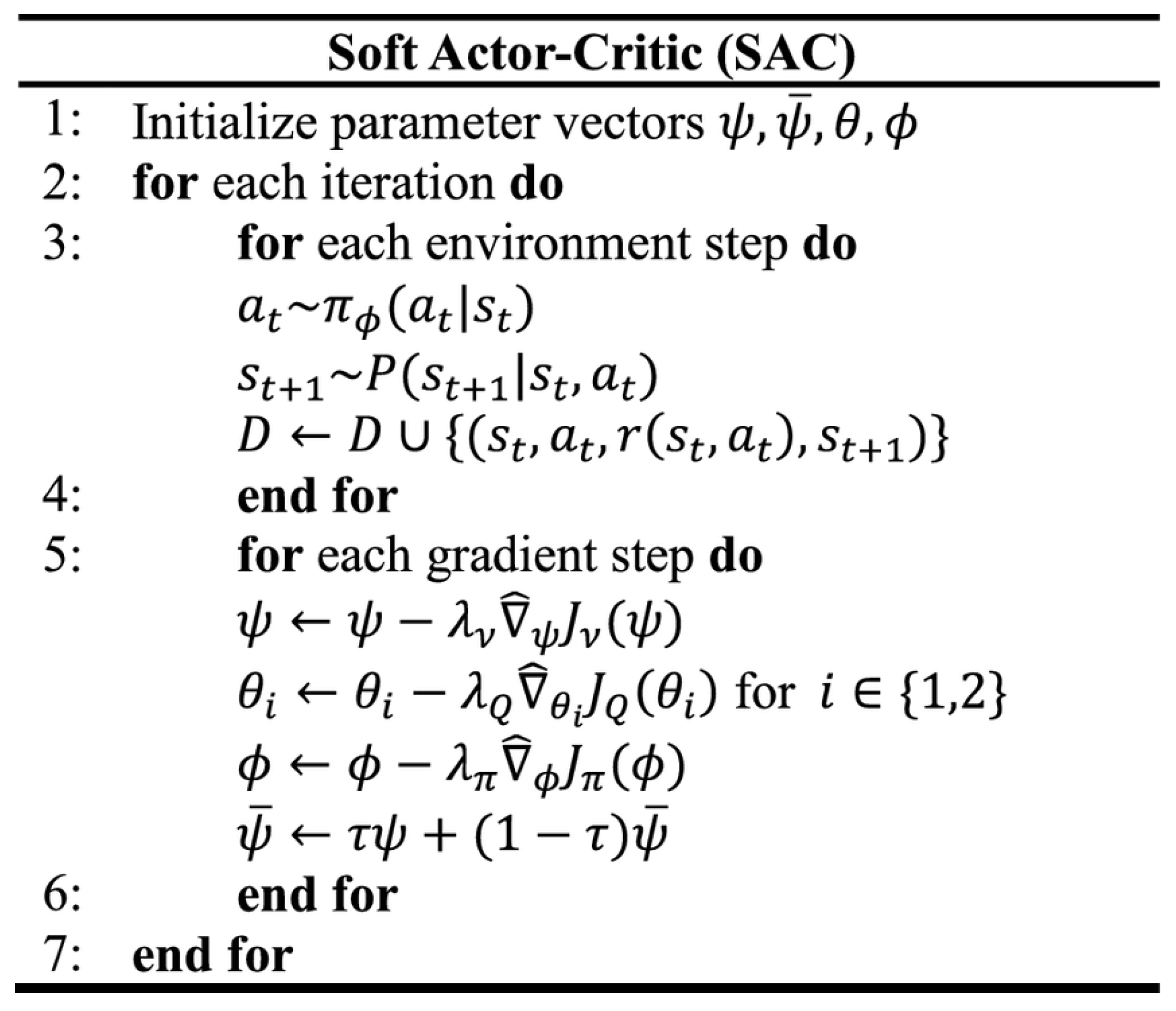
Regarding the continuous problem, we need a soft policy iteration method to calculate Q and , and use stochastic gradient descent for improvement. The SAC algorithm consists of three MLPs, representing the state value function, , the soft Q function, , and the policy, . The parameters are respectively. The objective functions for these three components, along with the SAC pseudo code (Figure 1) [8], are as follows:

Figure 1.
SAC pseudo code.
- Soft value function.represents the replay buffer of previously explored information. This function is used for stable training and assists in calculating the target Q function. Its gradient can be computed as shown in Equation (15). Actions must be selected according to the current policy, not from the replay buffer.
- Soft Q function.
- Policy update target.Adopting the reparameterization trick for action selection means that . Actions are sampled from a distribution, typically Gaussian, where outputs the mean and standard deviation, and is the noise. This allows for forming a distribution for sampling, enabling the gradient to be backpropagated through actions. The policy update objective function is shown in Equation (20).The problem with random sampling is that the action space is unbounded, while actions are usually a bounded number. To solve this, we use an invertible squashing function () to restrict actions to the range. The probability density function must also be corrected. Let be a random variable, then is its density, and the action is . The density becomes as shown in Equation (21).Equation (22) shows the correction needed for the action’s .Thus, the updated gradient is given by Equation (23).
3. Counteraction Simulation
3.1. Software Environments
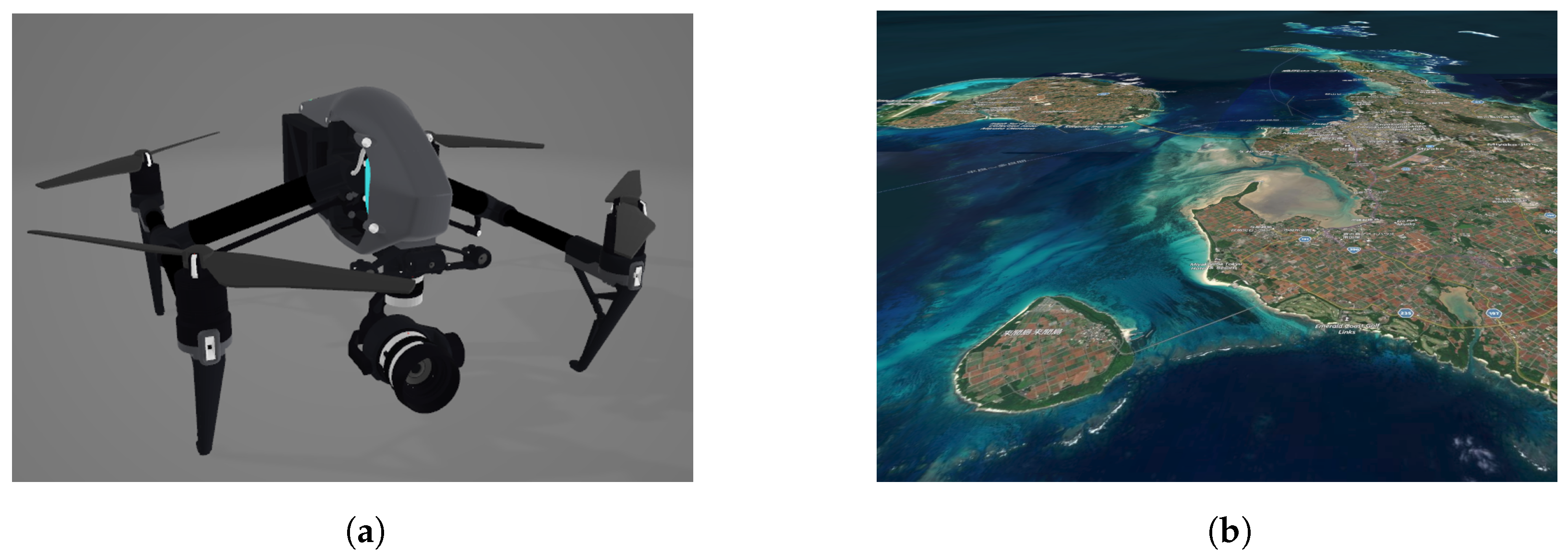
To achieve a near-realistic simulated environment, we used Unreal Engine for rendering scenes. It is a game engine developed by Epic Games for game development, movie effects, technology, and engineering. Unreal Engine also provides excellent physical simulations, such as object motion, collisions, and gravity. This makes it easier to gather information regarding impact determinations when performing versus game experiments. AirSim v1.8.1 from GitHub [22] was developed by Microsoft to study artificial intelligence and autonomous driving. It provides APIs in Python and C++ to obtain state and picture data, even when controlling the vehicle in the simulation. In summary, choosing Unreal Engine for the simulation of the drone combat and using AirSim’s drone control and physical modeling can reduce the real cost. In this study, we imported the model of the common commercial drone DJI Inspire series, as shown in Figure 2a.

Figure 2.
Drone modeling and environment. (a) Common commercial drone 3D models in AirSim. (b) Simulation of a island using CesiumJS.
In Unreal Engine, we used CesiumJS v1.111 from GitHub, which is an open source JavaScript library for creating world-class 3D globes and maps, and then imported it into Unreal Engine to build a 3D map. This helps us simulate combat in near-realistic terrain, as shown in Figure 2b.
3.2. Mission Scenario
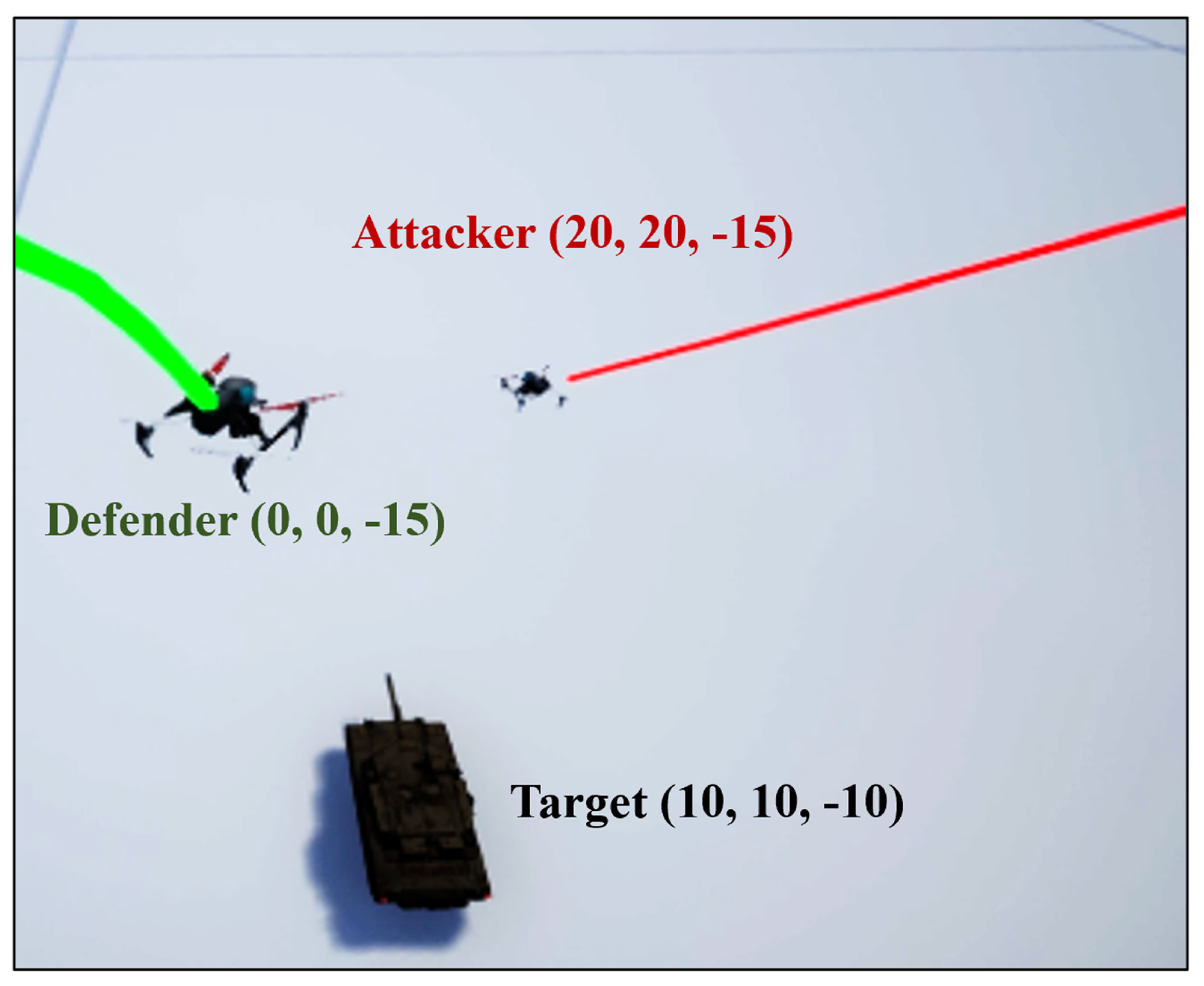
In this study, we used SAC to build a one-on-one drone counter game to verify the self-learning capability and robustness of the algorithm. After observing a real complex scene documentary video, a capture the flag game was adopted, as shown in Figure 3 and Figure 4. The green drone position indicates the starting point of the defender in meters. The red drone position was the starting point on the attacking side. The target (flag) was located in the air above the tank. The NED coordinate system was used for agents and world coordinates.

Figure 3.
Complex scene schematic in Unreal Engine.

Figure 4.
Deep reinforcement learning structure of counteraction.
The victory conditions of the attacker and the defender are listed in Table 1. Being within a specific range of the target airspace is required for an attacker to execute the bombing mission. It is necessary for the defender to approach the attacker and force it to retreat from the target airspace, or to be close enough to attack it. It is also possible to chase the target drone and force it to land; these three scenarios are used to determine the winner of each game.

Table 1.
Winning conditions.
As shown in Table 2, the states obtained by both sides correspond to the global position, velocity, and acceleration values (Ground Truth) provided by AirSim to validate the accuracy of the algorithm. There are 17 state values: the first 12 items are the movement state of the attacker and defender relative to the target, which represents the information that can be obtained about the target’s states. The 13th item is the result of the battle: one for land, two for win, three for loss, and four for exceeding the time limit of one game. Item 14 is the time from the start to the end of the game, with a maximum value of 50 as the time limit for a game, after which the game is over. Items 15–17 are the acceleration values, as listed in Table 3. AirSim already has a built-in drone dynamic model and control; therefore, the global speed is controlled by commands to simplify the complexity of the experiment. The outputs of the three actions, including the X, Y, and Z directions, are controlled by the SAC network, which ranges from −1 to +1.
Table 2.
SAC network reference states.
Table 3.
SAC network output action value.
3.3. Network
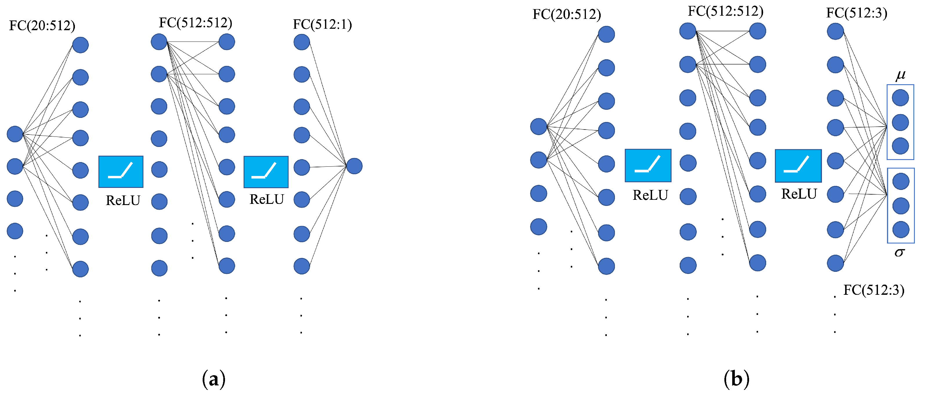
The attacker and defender use a set of SAC networks, as shown in Figure 5. The structures of the critic network and value network are shown in Figure 6a, which adopts the full connectivity layer and Rectified Linear Unit (ReLU) function. The inputs are 17 observations and three actions, and the outputs are Q or V. The structure of the actor network is shown in Figure 6b. Owing to the random strategy of SAC, the output are the mean and standard deviation of the three action values that are sampled to obtain the output of the action values.
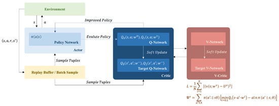
Figure 5.
Structure of SAC.

Figure 6.
Network schematic. (a) Critic network and value network. (b) Actor network.
The Adam Optimizer was used as a neural network optimizer because it is simpler to compute, more stable in gradient updating, and more widely used. It also has the advantages of a simple implementation, high efficiency, and stability. The network learning rate, value network update rate, and other parameters used in this chapter are listed in Table 4, and the parameters in the table are used as the experimental parameters after testing.
Table 4.
SAC network parameters.
4. Reward Function Optimization
One of the focuses of reinforcement learning is the design of reward functions. When an agent performs an action, it receives states and rewards from the environment and analyzes the value of the action based on them. The agent can achieve the desired goal more quickly and accurately by appropriately setting the reward function. Because this chapter uses two different SAC agents for reinforcement learning, they need to be designed for their respective purposes. The relative positions of the attacker and defender can be obtained by referring to states 1–3 in Table 2. The distance reward function, , is given by Equation (24). The closer the defender is to the attacker, the greater is the reward. If the defender remains at a certain distance, the reward value will be smaller. The relative position between the attacker and the target can be determined from states 7–9, and the distance reward function, , is designed as shown in Equation (25).
The distance reward function, , can also be determined through states 1–3, as shown in Equation (26). When the attacker is farther away from the defender, the deduction of the current reward value is reduced. If the attacker is too close to the defender, the penalty is stronger, forcing the attacker to move away from the defender. States 7 through 9 can be used to design the distance reward function, , as shown in Equation (27). When the attacker is farther from the target, the defender has a greater advantage. If the attacker gets too close to the target, the penalty for the defender increases dramatically.
States 10–12 indicate the agent’s velocity in relation to the target. In the case of an attacker, the velocity reward function, , is defined by Equation (28), which means that the relative position vector and velocity direction between attacker and target need to be the same. For example, if the target airspace is in front of the attacker, its velocity must face forward to obtain the reward. For the defender, the speed reward function, , is defined in the same manner. To obtain a higher reward, the defender has to fly towards the attacker, and, if it flies in the opposite direction away from the attacker, it will be punished as shown in Equation (29).
Using the same method, the velocity reward functions and can be defined as shown in Equations (30) and (31). When the attacker’s speed direction is not towards the target, the defender has an advantage, and, when the defender’s speed is towards the attacker, expulsion is achieved. The difference between Equations (28) and (29) is that the reward value is adjusted to 3. This implies that the attacker must aggressively attack the target to obtain a higher reward than passively avoiding the defender. The defender must approach an attacker more aggressively.
Referring to Table 2, state 13 records the final result of the game with reward , as shown in Equation (32).
State 14 is specified by a time-reward function, , as shown in Equation (33). The longer time it takes, the more the value of this reward increases negatively as the game time increases, which forces both players to engage in aggressive behavior.
In states 15–17, the acceleration reward function, , is designed as shown in Equation (34). Excessive acceleration during flight is likely to cause damage to mechanical devices, so it is added to make both sides fly at a smooth speed.
5. Results
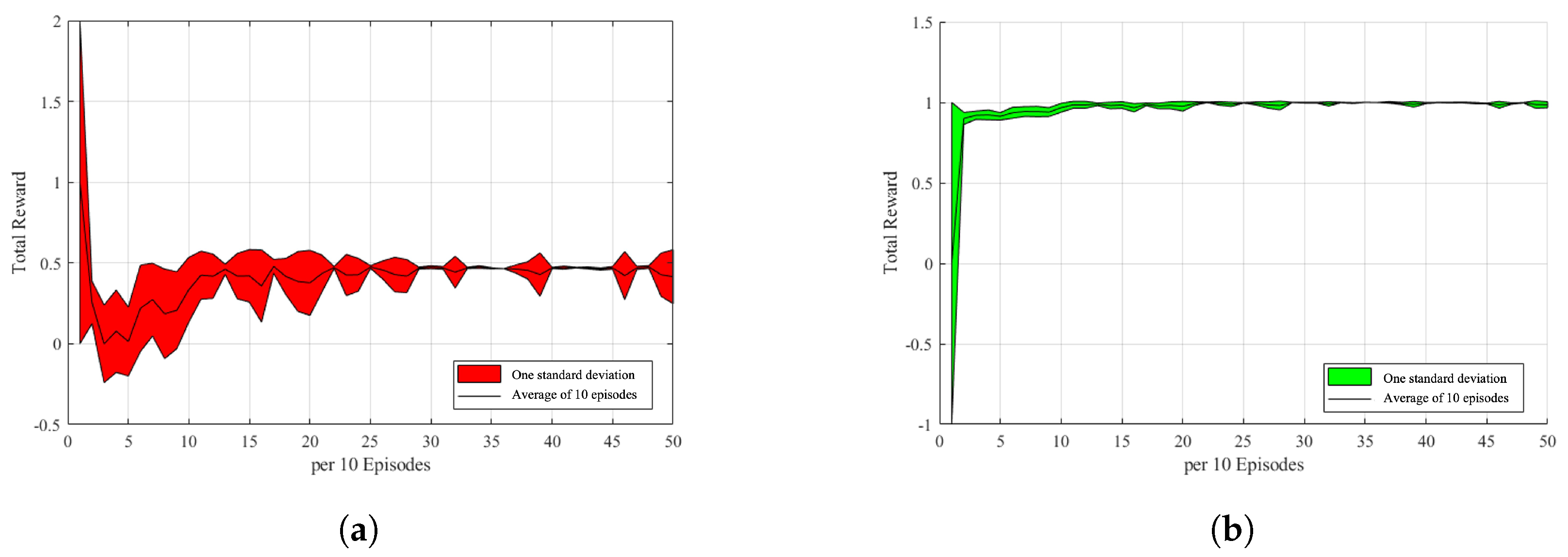
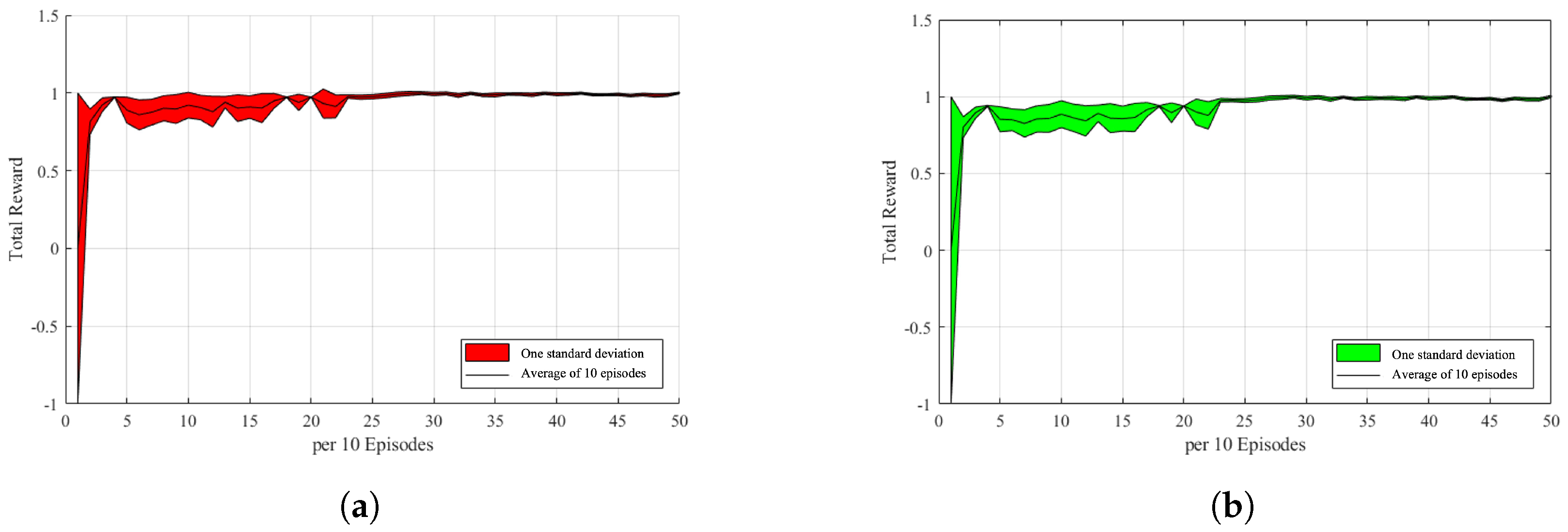
In this section, a game experimental simulation is introduced, which involves summing and recording the total rewards of a game from the environment setup and reward function design in Section 4. The lack of experience in the replay buffer allows both the attacker and the defender to perform random actions without training. The attacker and the defender obtain states, actions, and rewards from it until the accumulated experience exceeds the batch size before they start training. In this study, we computed the average of every 10 games, calculated the standard deviation of the data, and then mapped it to the range between −1 and 1 in Figure 7a,b. The black line in the graph is the average value, and the red or green part is the interval of the data with one standard deviation, which can be used to determine the stability of the network. For example, in Figure 7a, the larger the red area that covers the vertical interval is, the more unstable is the incentive value in that period. This may be due to the fact that the opponent is performing a rare behavior or the agent itself is trying other behaviors, resulting in a lower or higher reward value. As shown in Figure 7b, it can be observed that the defense is more stable, and it can be observed that, except for the initial phase, there are more volatile areas that correspond to the unstable areas of the attacker. This also indicates that the behavior of both sides will change owing to a change in the opponent’s strategy.

Figure 7.
Reward-episodes stats. (a) Attacker reward-episodes stats. (b) Defender reward-episodes stats.
The interactivity of both players’ behaviors was observed in the game, as shown in Figure 8. Because the target airspace position is a fixed value, it is easy for the attacker (red) to find a movement with a high reward value at the beginning of training. However, when an attacker increases its speed, it tends to miss the target position. This also leads to the need to return to nearby locations to explore the target position, resulting in an increased time cost and risk. With experience, the attacker learns to slow down at the right location, go under the target area first, and then increase the speed in the Z-axis direction to win the game.

Figure 8.
Attacker strategy. (Red line: Attacker. Green line: Defender.)
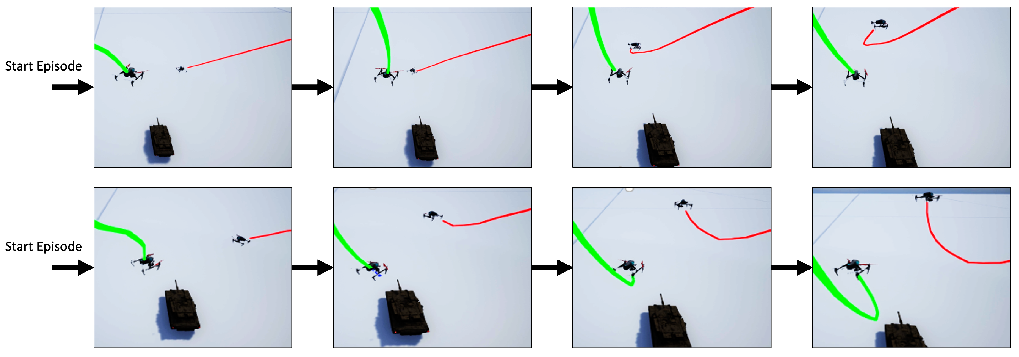
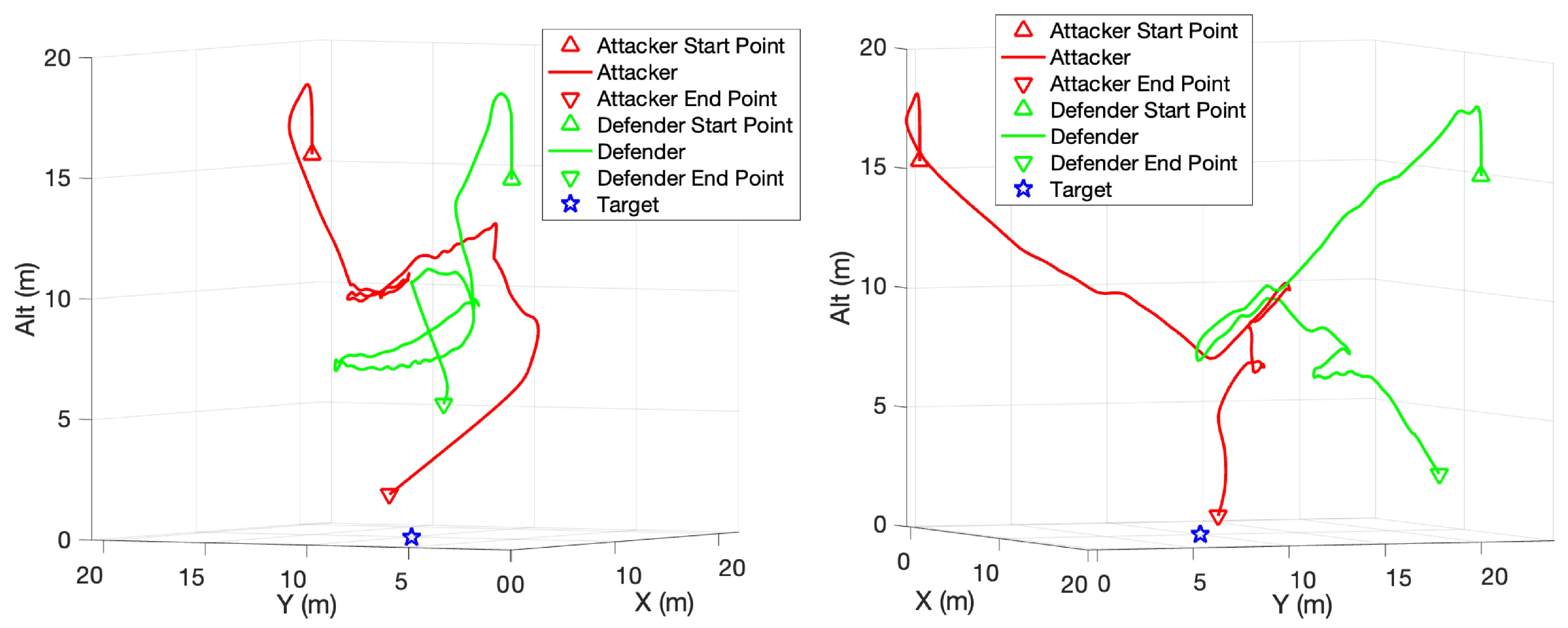
The defender (green) also learns the mobility of the quadcopter in a vertical climb during the game. Figure 9 shows two of these games, and it can be noticed that the defender also starts to use the fast pull-up for pursuit, which was frequently used in many games. The defender first enters the area below the attacker, and then approaches the attacker by pulling up vertically, increasing the speed of ascending while panning, and reducing the required time and distance. The path of the defender in the other two episodes are shown in Figure 10.
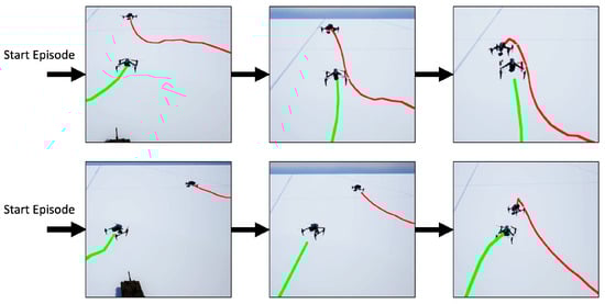
Figure 9.
Defender strategy. (Red line: Attacker. Green line: Defender.)

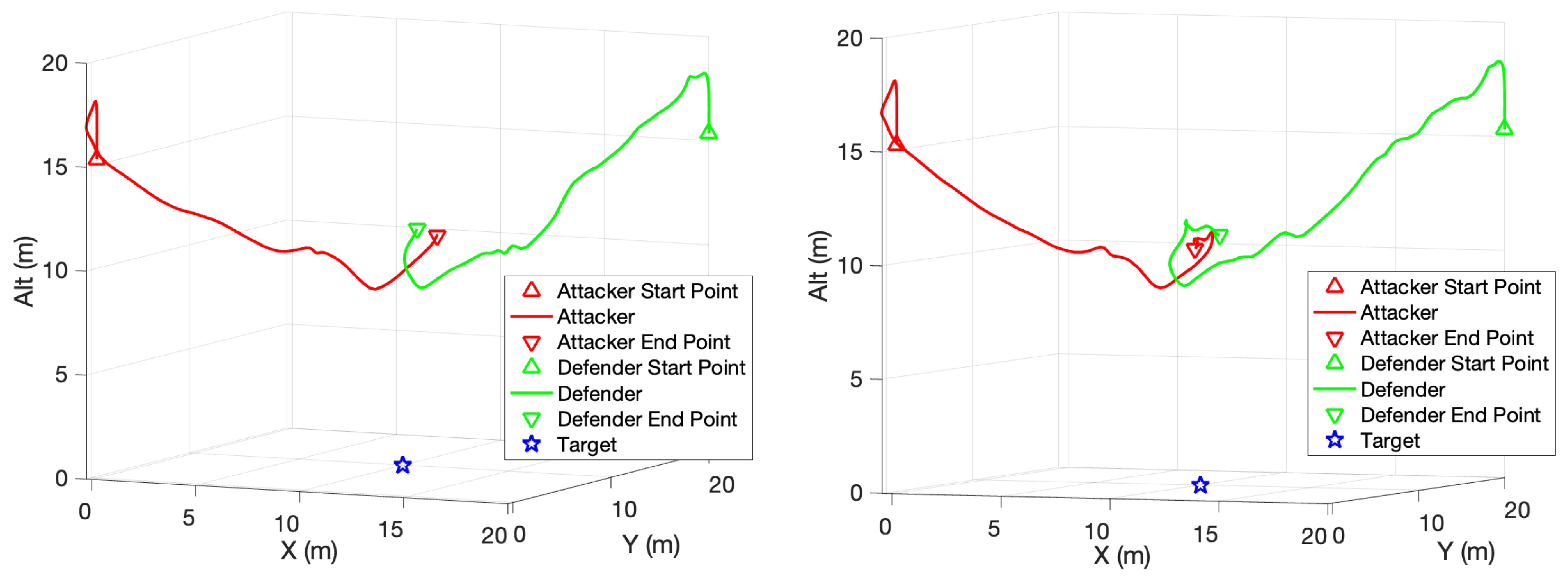
Figure 10.
Defender strategy path.
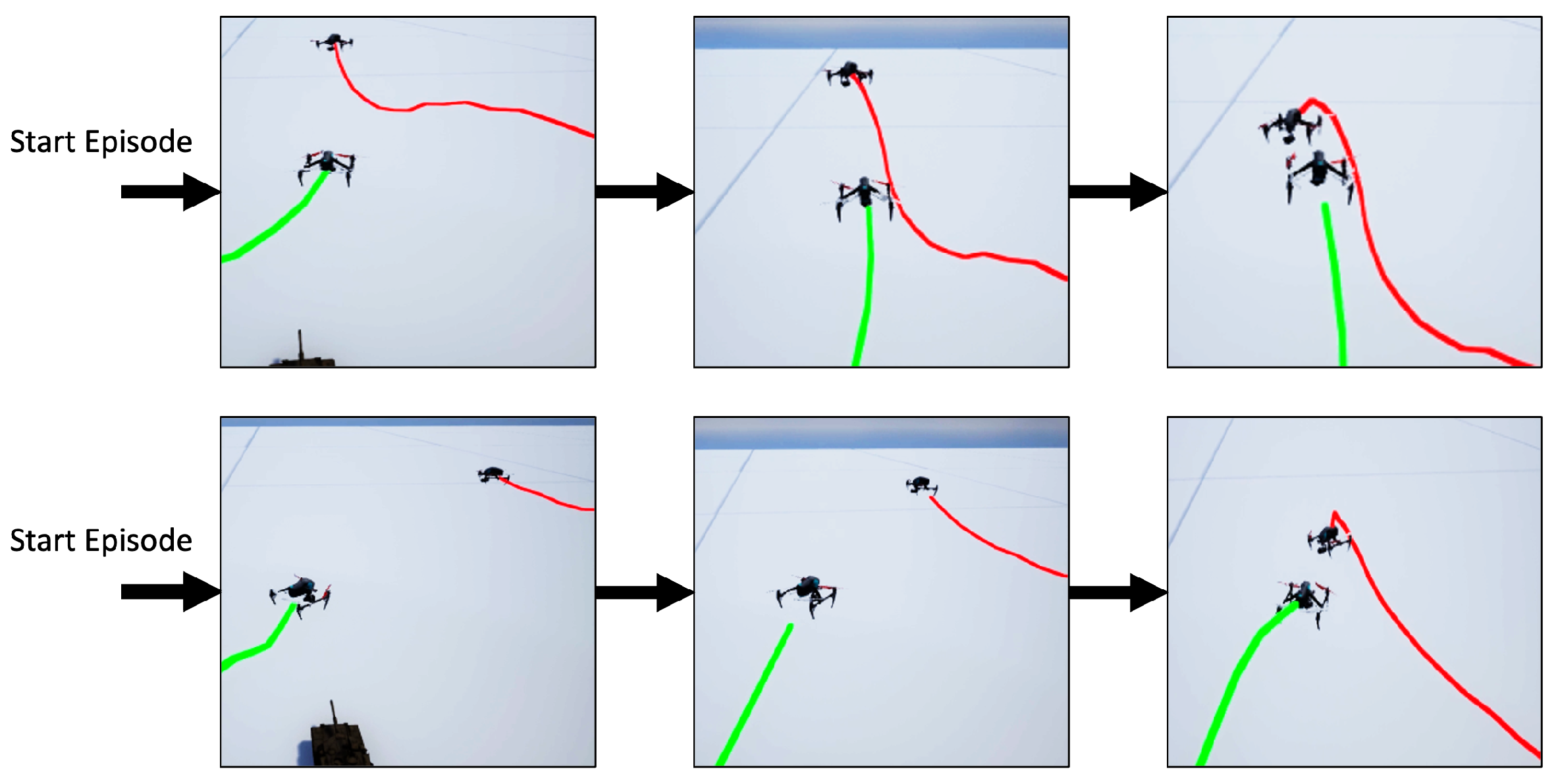
As the number of interceptions increases, the attacker begins to dodge the defender, as shown in Figure 11. As a comparison of Figure 8, the attacker tends to move away from the defender to avoid being intercepted when the defender approaches. It will start to climb even when it is far from the target, so it has a better chance of bypassing the defender and re-entering the target airspace. The path of the attacker in the other two episodes are shown in Figure 12.

Figure 11.
Enhanced attacker strategy. (Red line: Attacker. Green line: Defender).

Figure 12.
Enhanced attacker strategy path.
6. Discussion
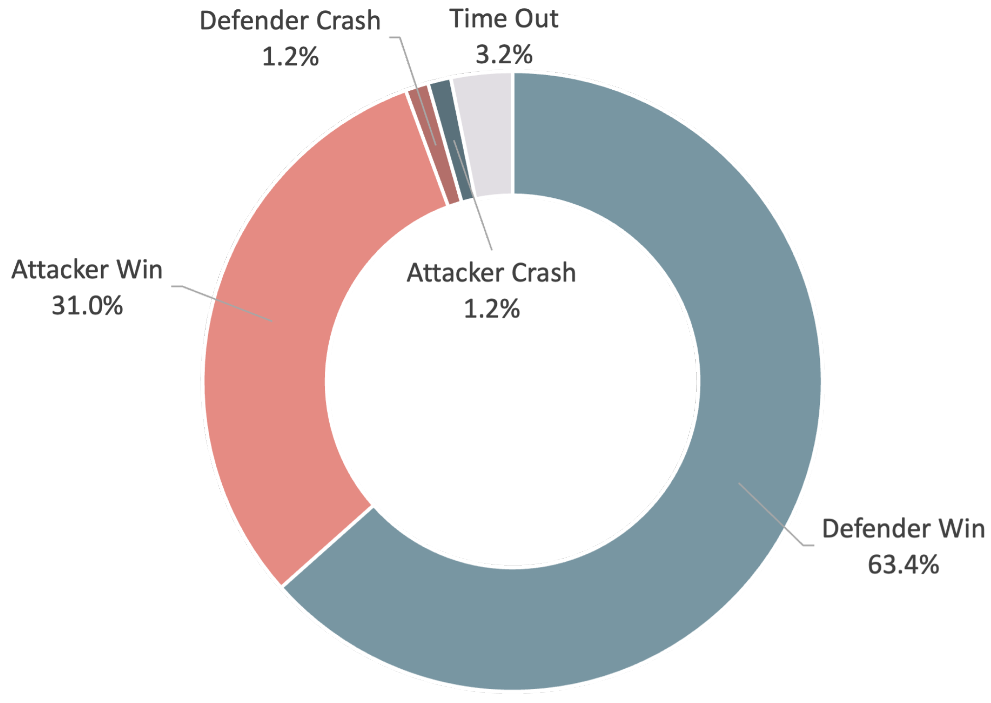
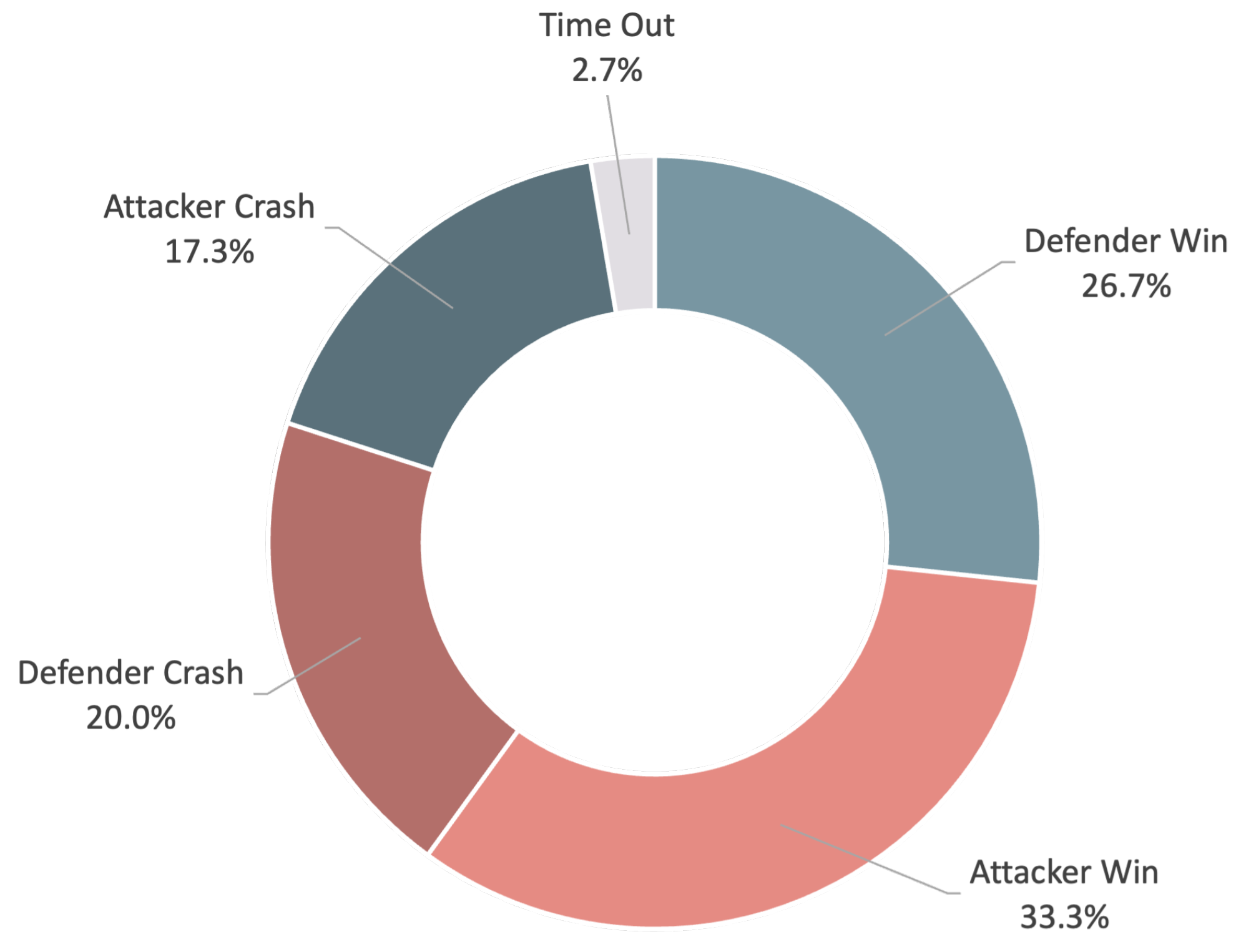
In total, 500 games were tested, and the results were analyzed, as shown in Figure 13. It can be found that the success rate of the attacker is only half of that of the defender, which may be due to the improper design of the attacker’s reward function. In Figure 7, it can be observed that the total rewards of the attacker are always much higher than those of the defender in all games. The high reward comes from the distance reward function, , associated with the target position, which is always greater than zero, making it difficult for the attacker to be effectively penalized in the course of its behavior. Therefore, the existing reward function can be modified to improve the attacker’s performance.

Figure 13.
Match results statistics.
As shown in Equation (37), the distance reward function, , is set such that the attacker is punished as long as the distance between the attacker and the target is not zero. As the distance increases, the penalty increases, which stimulates the agent to reduce the distance to the target in all directions to minimize the loss. Similarly, we can design the reward functions using Equation (38).
As shown in Equation (39), we define the distance reward functions . When the attacker is farther from the defender, the possibility of shooting down in the current state is lower. Therefore, maintaining a certain distance can reward the attacker. The farther the attacker is from the target, the more rewards the defender receives. The distance reward functions are shown in Equation (40). The other reward functions remained unchanged.
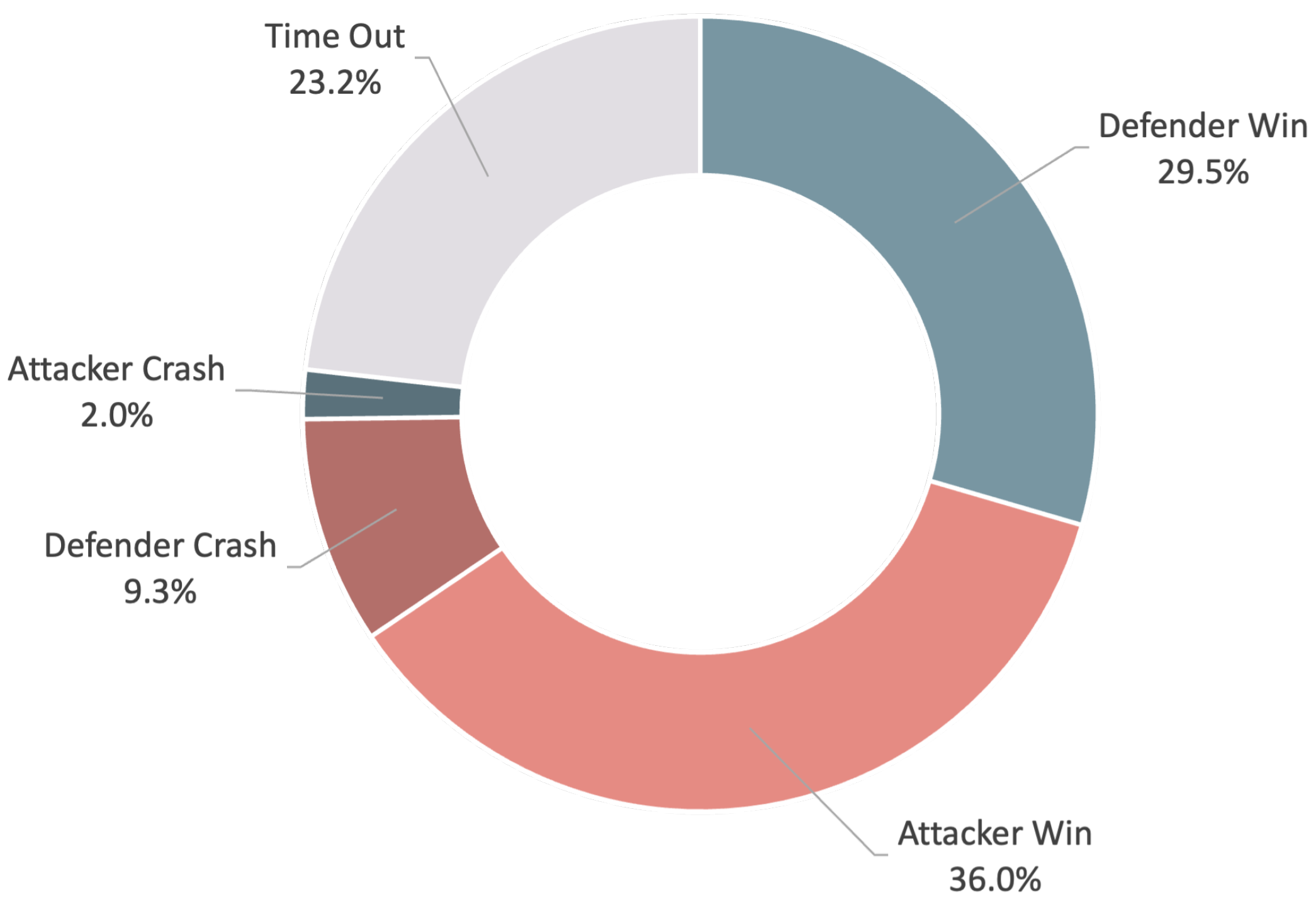
As shown in Figure 14, after the modification and initialization of the network weights, the total reward value of the attacker is still slightly higher than that of the defender. Because the absolute position of the target airspace is fixed, the attacker can find high-value movements faster than the defender and achieve a higher win rate in the early stage, as shown in Figure 14a. Moreover, the attacker’s network is stabilized compared with the late stage, as shown in Figure 7. As shown in Figure 15, the results of the 500 tested games show that the success and tie rates of the attacker also increased significantly. This implies that the reward function setting is very important for enhancing the stability of learning and results.

Figure 14.
Reward-episodes stats. (a) Attacker reward-episodes stats. (b) Defender reward-episodes stats.

Figure 15.
Match results statistics.
The adaptability of the SAC trained network to different scenarios is tested by a change of attacker initial position and target location, where the attacker’s initial position and target location are changed to and , respectively. The initial position of the defender remains the same. The statistical results of 500 games are shown in Figure 16. This shows that a change of relative positions between one another affects the winning rate of both sides. The winning rate of the defender increases from 31.5% to 45.3%, and the attacker’s winning rate increases from 45.3 to 53.3%. This reveals that a change of initial position does not always lower the winning rate, and the initial condition may confer an advantage when performing a mission. These results show that the network trained by the SAC algorithm has adaptability to different scenarios in terms of keeping a winning rate around or above 30% for both sides.

Figure 16.
Attacker’s position , and target’s position .
7. Conclusions
This study proposed an SAC architecture to enable a drone to learn how to approach a target without being intercepted by a defender drone in versus games, and, in the same way, to enable a drone to learn how to intercept an invasive drone and to protect ground-friendly teammates. By providing an action pool for performing acceleration, bypassing, and dodging, drones can learn the tactical skills required to achieve the mission through a series of game scenarios. The results demonstrate that a proper reward provides appropriate incentives and motivates the drone to explore highly rewarded actions. In the one-on-one game scenarios, the tie rate increased from 3.2% to 23.2% after the reinforcement learning process. The attacker–defender winning ratio also improved from 1:2 to 1.2:1. Both attackers and defenders are evenly matched after adjusting the reward, which is reasonable for drones with equal flight capabilities.
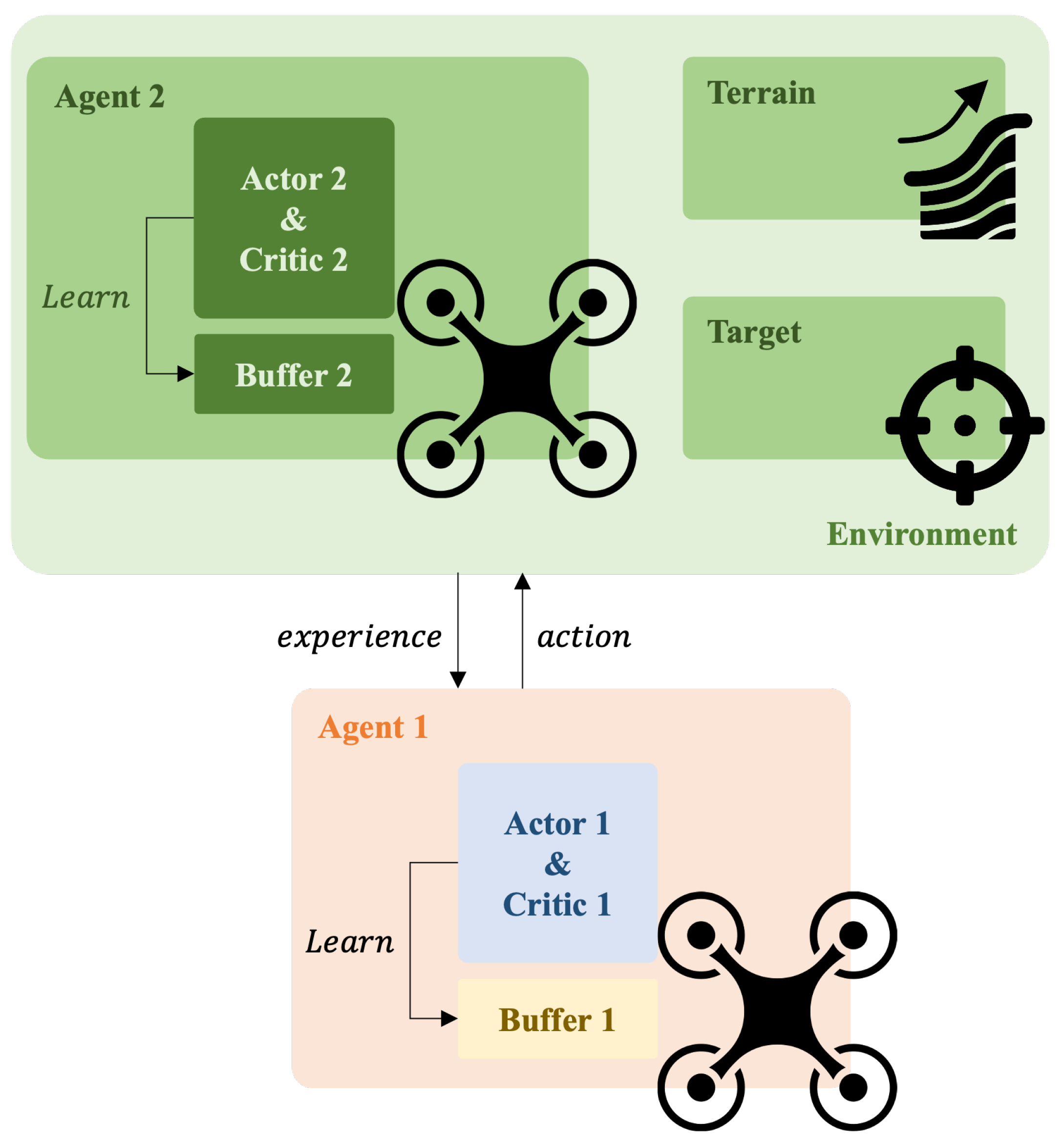
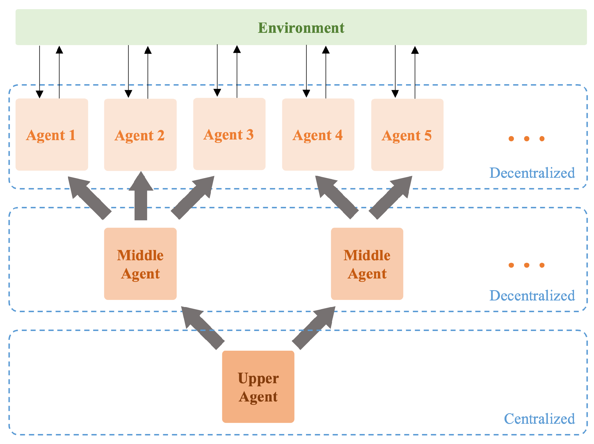
For complex scenarios and requirements, such as many-to-many versus, future approaches will combine decentralized and centralized methods to overcome the limitations of each architecture and achieve higher efficiency and results. The schematic diagram of the architecture is shown in Figure 17. The system will be divided into hierarchical modes, with each layer organized in a decentralized or centralized manner based on the requirements. In this setup, each agent retains a decentralized decision-making approach concerning the environment. This means they maintain autonomous action policies and make independent decisions based on the local information they obtain. At this level, the information between agents can be decentralized, and it does not necessarily require the environmental information obtained by other agents. Even if some agents are lost, this will not affect the operation of this layer. The intermediate strategy selection layer functions as a transition from local decisions to the upper agent. It can be viewed as a small cluster of agent nodes that formulate strategies for a certain number of agents based on commands from the upper layer and local information. Practically, sub-task modes can be inserted at this level. These sub-tasks are decentralized, meaning the interactions between different sub-tasks are minimized. At this point, multiple agents can be assembled under each sub-task, sharing environmental information and achieving the sub-task’s goals through centralized coordination. The upper agent is the central controller, which collects and organizes all environmental information, observes the state of the entire system, and makes the highest-level decisions. In addition to performing learning and optimization, it commands the intermediate sub-tasks to accomplish the final mission requirements.

Figure 17.
Hierarchical multi-agent architecture.
In many-to-many confrontations, future approaches will involve training individual strategies based on different combinations of offensive and defensive engagements, as illustrated in Figure 18. For example, the current scenario could be three versus three, three versus two, or two versus three. During execution, the large and complex system state will be decomposed into subsystems that can communicate and coordinate with each other, making the system more manageable and robust. In the learning simulation process, a reward scoring mechanism needs to be established to indicate the advantages and disadvantages of the current state. Based on this analysis, pre-designed and well-trained action modes will be switched to action accordingly. This approach is similar to how athletes break down the skills required for a match into individual training sessions and decide which strategies to employ during the game based on the current situation to gain an advantage.
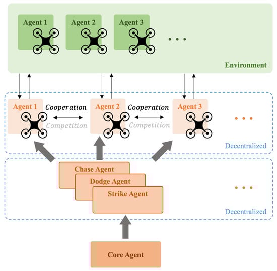
Figure 18.
Many-to-many confrontation architecture.
Author Contributions
Conceptualization, C.-L.C. and Y.-W.H.; methodology, C.-L.C. and Y.-W.H.; software, Y.-W.H.; validation, C.-L.C.; formal analysis, Y.-W.H.; data curation, T.-J.S.; writing—original draft preparation, Y.-W.H.; writing—review and editing, C.-L.C. and T.-J.S.; supervision, C.-L.C.; funding acquisition, C.-L.C. All authors have read and agreed to the published version of the manuscript.
Funding
Part of this work was supported by The Armaments Bureau, MND and the Ministry of Science and Technology under Grant No. MOST 109-2221-E-006-007.
Institutional Review Board Statement
Not applicable.
Informed Consent Statement
Not applicable.
Data Availability Statement
No new data were created.
Conflicts of Interest
The authors declare no conflicts of interest.
References
- Watkins, C.J.; Dayan, P. Q-learning. Mach. Learn. 1992, 8, 279–292. [Google Scholar] [CrossRef]
- Hosu, I.A.; Rebedea, T. Playing atari games with deep reinforcement learning and human checkpoint replay. arXiv 2016, arXiv:1607.05077. [Google Scholar]
- Mnih, V.; Kavukcuoglu, K.; Silver, D.; Graves, A.; Antonoglou, I.; Wierstra, D.; Riedmiller, M. Playing atari with deep reinforcement learning. arXiv 2013, arXiv:1312.5602. [Google Scholar]
- Lillicrap, T.P.; Hunt, J.J.; Pritzel, A.; Heess, N.; Erez, T.; Tassa, Y.; Silver, D.; Wierstra, D. Continuous control with deep reinforcement learning. arXiv 2015, arXiv:1509.02971. [Google Scholar]
- Gu, S.; Lillicrap, T.; Sutskever, I.; Levine, S. Continuous deep q-learning with model-based acceleration. In Proceedings of the International Conference on Machine Learning, PMLR, New York, NY, USA, 20–22 June 2016; pp. 2829–2838. [Google Scholar]
- Gu, S.; Holly, E.; Lillicrap, T.P.; Levine, S. Deep reinforcement learning for robotic manipulation. arXiv 2016, arXiv:1610.00633. [Google Scholar]
- Wang, Y.; Huang, C.; Tang, C. Research on unmanned combat aerial vehicle robust maneuvering decision under incomplete target information. Adv. Mech. Eng. 2016, 8, 1687814016674384. [Google Scholar] [CrossRef]
- Haarnoja, T.; Zhou, A.; Abbeel, P.; Levine, S. Soft actor-critic: Off-policy maximum entropy deep reinforcement learning with a stochastic actor. In Proceedings of the International Conference on Machine Learning, PMLR, Stockholm, Sweden, 10–15 July 2018; pp. 1861–1870. [Google Scholar]
- Haarnoja, T.; Zhou, A.; Hartikainen, K.; Tucker, G.; Ha, S.; Tan, J.; Kumar, V.; Zhu, H.; Gupta, A.; Abbeel, P.; et al. Soft actor-critic algorithms and applications. arXiv 2018, arXiv:1812.05905. [Google Scholar]
- Kurniawan, B.; Vamplew, P.; Papasimeon, M.; Dazeley, R.; Foale, C. An empirical study of reward structures for actor-critic reinforcement learning in air combat manoeuvring simulation. In Proceedings of the Australasian Joint Conference on Artificial Intelligence, Adelaide, Australia, 2–5 December 2019; Springer: Berlin/Heidelberg, Germany, 2019; pp. 54–65. [Google Scholar]
- Yang, Q.; Zhu, Y.; Zhang, J.; Qiao, S.; Liu, J. UAV air combat autonomous maneuver decision based on DDPG algorithm. In Proceedings of the 2019 IEEE 15th International Conference on Control and Automation (ICCA), Edinburgh, Scotland, 16–19 July 2019; IEEE: Piscataway, NJ, USA, 2019; pp. 37–42. [Google Scholar]
- Lei, X.; Dali, D.; Zhenglei, W.; Zhifei, X.; Andi, T. Moving time UCAV maneuver decision based on the dynamic relational weight algorithm and trajectory prediction. Math. Probl. Eng. 2021, 2021, 1–19. [Google Scholar] [CrossRef]
- Pope, A.P.; Ide, J.S.; Mićović, D.; Diaz, H.; Rosenbluth, D.; Ritholtz, L.; Twedt, J.C.; Walker, T.T.; Alcedo, K.; Javorsek, D. Hierarchical reinforcement learning for air-to-air combat. In Proceedings of the 2021 International Conference on Unmanned Aircraft Systems (ICUAS), Athens, Greece, 15–18 June 2021; IEEE: Piscataway, NJ, USA, 2021; pp. 275–284. [Google Scholar]
- Pope, A.P.; Ide, J.S.; Mićović, D.; Diaz, H.; Twedt, J.C.; Alcedo, K.; Walker, T.T.; Rosenbluth, D.; Ritholtz, L.; Javorsek, D. Hierarchical Reinforcement Learning for Air Combat At DARPA’s AlphaDogfight Trials. IEEE Trans. Artif. Intell. 2022, 4, 1371–1385. [Google Scholar] [CrossRef]
- Zheng, J.; Ma, Q.; Yang, S.; Wang, S.; Liang, Y.; Ma, J. Research on cooperative operation of air combat based on multi-agent. In Proceedings of the International Conference on Human Interaction and Emerging Technologies, Virtual, 27–29 August 2020; Springer: Berlin/Heidelberg, Germany, 2020; pp. 175–179. [Google Scholar]
- Zhou, K.; Wei, R.; Xu, Z.; Zhang, Q. A brain like air combat learning system inspired by human learning mechanism. In Proceedings of the 2018 IEEE CSAA Guidance, Navigation and Control Conference (CGNCC), Xiamen, China, 10–12 August 2018; IEEE: Piscataway, NJ, USA, 2018; pp. 1–6. [Google Scholar]
- Zhou, K.; Wei, R.; Xu, Z.; Zhang, Q.; Lu, H.; Zhang, G. An air combat decision learning system based on a brain-like cognitive mechanism. Cogn. Comput. 2020, 12, 128–139. [Google Scholar] [CrossRef]
- Zhou, K.; Wei, R.; Zhang, Q.; Xu, Z. Learning System for air combat decision inspired by cognitive mechanisms of the brain. IEEE Access 2020, 8, 8129–8144. [Google Scholar] [CrossRef]
- Kong, W.; Zhou, D.; Yang, Z.; Zhao, Y.; Zhang, K. UAV autonomous aerial combat maneuver strategy generation with observation error based on state-adversarial deep deterministic policy gradient and inverse reinforcement learning. Electronics 2020, 9, 1121. [Google Scholar] [CrossRef]
- Sun, Z.; Piao, H.; Yang, Z.; Zhao, Y.; Zhan, G.; Zhou, D.; Meng, G.; Chen, H.; Chen, X.; Qu, B.; et al. Multi-agent hierarchical policy gradient for air combat tactics emergence via self-play. Eng. Appl. Artif. Intell. 2021, 98, 104112. [Google Scholar] [CrossRef]
- Sutton, R.S.; Barto, A.G. Reinforcement Learning: An Introduction; MIT Press: Cambridge, MA, USA, 2018. [Google Scholar]
- Shah, S.; Dey, D.; Lovett, C.; Kapoor, A. AirSim: High-Fidelity Visual and Physical Simulation for Autonomous Vehicles. In Proceedings of the Field and Service Robotics, Zurich, Switzerland, 12–15 September 2017; Available online: http://xxx.lanl.gov/abs/arXiv:1705.05065 (accessed on 15 December 2022).


Disclaimer/Publisher’s Note: The statements, opinions and data contained in all publications are solely those of the individual author(s) and contributor(s) and not of MDPI and/or the editor(s). MDPI and/or the editor(s) disclaim responsibility for any injury to people or property resulting from any ideas, methods, instructions or products referred to in the content. |
© 2024 by the authors. Licensee MDPI, Basel, Switzerland. This article is an open access article distributed under the terms and conditions of the Creative Commons Attribution (CC BY) license (https://creativecommons.org/licenses/by/4.0/).